Abstract
Increasingly, Chinese cities are proposing city-scale ventilation corridors (VCs) to strengthen wind velocities and decrease pollution concentrations, although their influences are ambiguous. To assess VC impacts, an effort has been made to predict the impact of VC solutions in the high density and diverse land use of the coastal city of Shanghai, China, in this paper. One base scenario and three VC scenarios, with various VC widths, locations, and densities, were first created. Then, the combination of the Weather Research and Forecasting/Single-Layer Urban Canopy Model (WRFv.3.4/UCM) and Community Multiscale Air Quality (CMAQv.5.0.1) numerical simulation models were employed to comprehensively evaluate the impacts of urban spatial form and VC plans on PM2.5 concentrations. The modeling results indicated that concentrations increased within the VCs in both summer and winter, and the upwind concentration decreased in winter. These counter-intuitive results could be explained by decreased planetary boundary layer (PBL), roughness height, deposition rate, and wind speeds induced by land use and urban height modifications. PM2.5 deposition flux decreased by 15–20% in the VCs, which was attributed to the roughness height decrease for it weakens aerodynamic resistance (Ra). PBL heights within the VCs decreased 15–100 m, and the entire Shanghai’s PBL heights also decreased in general. The modeling results suggest that VCs may not be as functional as certain urban planners have presumed.
1. Introduction
Chinese cities have proposed varieties of urban plans, strategies, and management plans in response to severe intra-urban fine particulate (PM2.5) pollution in past years [,]. Among them, city-scale ventilation corridors (VCs) are an aggressive but popular proposal []. Certain megacities, such as Shanghai, Beijing, and Nanjing, have started to plan urban VCs to mitigate air pollution concentrations. The assumption behind the VC plans is that VCs can alleviate pollution levels by increasing wind velocity and pollution dispersions. However, the urban-scale VCs have not been well identified, although there have been many references studying the street canyon’s effects on air pollution variations [,,]. The VCs’ influence on urban ventilation and air pollution needs to be adequately evaluated to support plans and implementations. Therefore, this paper, as one of the earliest attempts, investigates VC’s effectiveness on air pollution influences at the urban level.
Urban VCs did not have rigorous definitions prior to this work and were defined as continuous low-rise zones of highways, waterways, parks, and/or vacant lands in urban areas in this paper. The well-developed term of ‘ecological corridor’ (EC) has similar definitions to the VC, but EC-related studies have primarily focused on the corridor’s ecological services regarding biodiversity, wetlands, and urban heat island effects (UHI) []. There exist micro-level (street, neighborhood) and macro-level (city, region) VCs, and different scales should be employed for the respective approaches. Site campaigns and computational fluid dynamics (CFD) are common methods in micro-scale studies []. Site campaigns need intensive field measurements, and CFD requires a large amount of computation. The micro-scale studies performed well because of intensive laboring measurements and/or computer processing, but it is challenging to apply to macro-scales under current computing conditions and labor rates. Hence, statistical analysis using data released from standard monitor networks (e.g., Land Use Regression, GAMs), remote sensing, or mid-macro level simulations (WRF, MM5, CMAQ) are widely used in city and regional studies [,,]. The statistical methods were usually limited by sparse monitors: there are only 30 to 50 monitors located in megacities. Thus, the results from statistical methods omit certain local variations when developing spatial analysis. Remote sensing technology and middle-macro (city scale to global scale) simulations both overcome the data unavailability problem and can be used to predict fine-scale pollution variations []. Remote sensing could supply high-quality land-use maps and elevation maps, which are the basis for VC planning and design. Remote sensing by itself cannot predict meteoritical responses when there is land-use change, so incorporation with middle-macro meteorological and air-polluting simulation approaches can investigate the VCs’ effects.
A set of middle-macro models can be used to simulate urban wind field and intra air pollution emissions and dispersions under different landforms and meteorology [,,,]. Two widely used packages to simulate multiscale climate are Weather Research and Forecasting (WRF) and Community Multiscale Air Quality (CMAQ). WRF is powerful at simulating regional to national level meteorological performance, and urban areas are usually treated the same as rural areas. As the cities’ distinguishing characteristics, such as high building density, were not considered, an extended urban canopy model (WRF-UCM) was developed to specify urban area simulation; it received better results compared to the general WRF approach []. The major difference is that the WRF-UCM model has more categories of land use (low-residential, high residential, and commercial–industrials), with corresponding surface parameters.
WRF/UCM models have become increasingly used in urban areas to model spatial meteorology in cities [,,,]. Although there have been very few studies using WRF-UCM to estimate the ventilation change before and after urban planning, there have been certain references exploring the heat island effect before/after plans. Papangelis et al. [] utilized WRF-UCM to learn about the thermal effects induced by “green plans”. An urban park (8 km × 4 km) was designed in the City of Athens, Greece, and modeled. The results indicated that significant cooling effects would exist at night after the green plans are adopted. WRF-UCM is qualified to model and compare meteorology variances induced by urban plans []. Therefore, we also employed WRF v.3.4-UCM in this paper to model wind field change due to VCs.
The most used package to simulate air pollution at the city level is the CMAQ package developed by the EPA of the US []. Many studies have proved its strong predicting capacity both in China and worldwide [,,]. Therefore, CMAQ v.5.0.1 was chosen to simulate air pollution concentrations before and after VC plans incorporating the climate data from WRF.
In conclusion, there have been few studies assessing the effects of urban VC planning on urban wind fields and PM2.5 concentrations. Without solid evaluation, the ambitious government VC plans lack evidence and cannot persuade the public and scholars. Based on the gap, this paper proposes a new framework to estimate the VC impacts on ventilation and air pollution to support policy-making.
2. Methods
Three VC scenarios were created to investigate the effects of VCs based on Shanghai’s existing land use, ecological plan, and prevailing wind directions. VC plans differed from the status quo on city morphology and land uses. Then, customized morphology of the city, representing building heights and land use, was used to generate an urban wind field map in WRFv.3.4-UCM. Based on studies by Briggs et al. [] and Liu et al. [], meteorological data of about 2 weeks can avoid the negative effects of sudden weather changes so that they are enough for modeling. Thus, ventilation records from two monitors for the dates of 1–15 July 2014 and 1–15 December 2014 were used to calibrate and evaluate the WRF outputs. Then, PM2.5 pollution maps were created in CMAQv.5.0.1, incorporating the meteorology map generated with WRFv.3.4-UCM. The results of PM2.5 pollution from CMAQv.5.0.1 were also evaluated against the same monitors’ pollution records. Then, each VC scenario was assessed by WRFv.3.4-UCM and CMAQv.5.0.1 to simulate PM2.5 values within VCs and the whole city. Finally, using a comparison between PM2.5 pollution in Shanghai’s base scenario and VC planning scenarios, the performance of VCs was summarized and analyzed. The above research flow is shown in Figure 1.
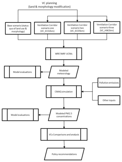
Figure 1.
Flow chart of the research on the VCs’ effects on PM2.5 pollution on an urban scale.
2.1. Case Study Area and Observed Data
The City of Shanghai, China, was chosen to elaborate the research approach. Data from 12 PM2.5 monitors in the city center and suburban areas were collected by Shanghai Environmental Monitor Center and used in the analysis. These PM2.5 monitors did not record meteorology-related data; thus, other data sources needed to be cited for meteorology. Meteorological data, including wind speed, temperature, pressure, wind direction, and humidity, were recorded from two airport stations (Hongqiao and Pudong) (Figure 2a) in the Automated Surface Observing System (ASOS) network. The data period was in the summer and winter of 1–15 July 2014 and 1–15 December 2014. Shanghai base land use data for modeling was drawn in 2011 by the Shanghai government, with resolutions of about 100 m in the city center and about 1000 m in suburban areas. Figure 2b shows the 10major land-use types in the Shanghai base map.
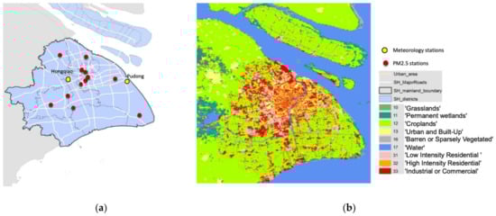
Figure 2.
(a) Shanghai area map and meteorology/PM2.5 monitor locations; (b) 10 base land uses of the city of Shanghai.
2.2. VC Planning Scenarios
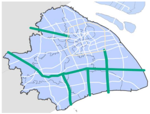
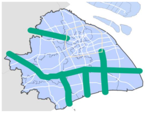
Three VC scenarios were planned, surrounding highways, high-density buildings, and existing or planned ecological areas (Table 1). In all these scenarios, the land within VCs was assumed to be grass, and the emissions were kept the same as the base scenario, which means this research only tests the dispersion effects of the VCs, not the removal effects. Keeping the same emission inventory and population in the base and VC scenarios may not be realistic because green lands usually do not have emission sources in practice. However, it makes the urban average concentration comparison more persuasive with the unchanged emission amount. In the VC scenarios, we set the height of all the VC areas to 0 m for grasslands and kept other areas the same as the base scenario Global Digital Elevation Model (GDEM) file. The decrease in height (including building heights) was 20–50 m in built-up areas and 0–10 m in other areas (Figure 3).

Table 1.
VC planning scenarios and explanations.
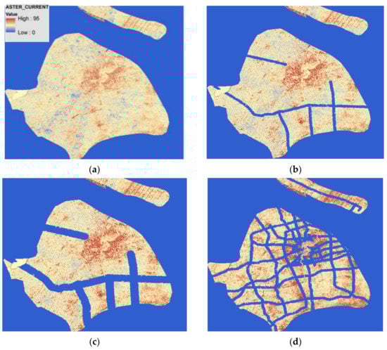
Figure 3.
Base and VC morphology maps of Shanghai, China: (a) base; (b) VC_ECO2KM; (c) VC_ECO5KM; (d) VC_HW2KM.
There are four basic rules for creating VC planning scenarios: current land use status, Shanghai municipal ecological plan, prevailing wind, and highway buffer effect. The VC planning areas contain both high-density urban lands (e.g., the north-west corridor in the ECO_2KM scenario) and low-density suburban lands (e.g., the south corridors in the ECO_2KM scenario). VCs in different locations can test impact differences caused by land density and use.
The Shanghai Municipal Administration of Planning and Land Resource published an ecological protective zone plan in 2020. Figure 4 is the planning map in which the green areas are different ecological zones restricted from urban development. In this plan, the green corridors are mainly located in suburban areas, along with rivers and major roads. Following this plan, we extracted several major green corridors and simplified them to the VCs (Table 1).
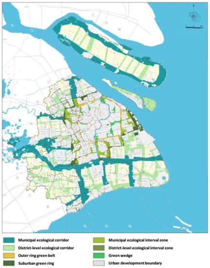
Figure 4.
Shanghai Ecological Protective Plan (draft version) in 2020 [].
Shanghai’s wind fields were also considered in the VC plans. Studies have found that VCs parallel to wind directions usually have larger horizontal ventilation effects, thus decreasing pollution concentration, and VCs perpendicular to wind directions usually have turbulent mixing effects, thus increasing pollution concentration []. Wind from the north is identified as the prevailing wind in winter, while that in summer is from the southeast in Shanghai. The corridors from northeast and southwest directions, which are parallel to the dominant winds, should be the best of all directions for increasing ventilation speeds, according to previous studies [].
In addition, highway buffers were treated as potential VCs because the buffers could alleviate human exposure to the transportation-emitted pollutants if residents did not live in these buffers.
In conclusion, the conceptual VC scenarios were created under considerations of the status quo of land use, ecological zones planned by the government, and wind conditions. There are many limitations to implementing these plans even when their concentration mitigating effects are significant. However, these conceptual VC plans, with various features of land use, building density, location, and width, are appropriate for estimating different VC influences.
2.3. The WRF-UCM Modeling System
Meteorological change before (base scenario) and after (VC scenarios) urban VC plans was modeled by the Weather Research and Forecasting (WRF 3.9) model, incorporating the Single-Layer Urban Canopy Model (UCM) in this study. WRF was developed by the National Center for Atmospheric Research (NCAR) for a broad range of applications across scales. It consists of four major parts: the WRF Preprocessing System (WPS), (optional) WRF Data Assimilation (WRF-DA), the Advanced Research WRF-ARW solver, and post-processing and visualization tools. Regional scale is the WRF’s primary study scope, while urban climate that is influenced by complicated land use and morphology is not primarily considered its modeling objective. An expanded module, WRF-UCM, was then designed specifically for simulating meteorology in urban areas []. The core differences of the WRF-UCM to WRF include (1) urban canopy parameterization schemes, (2) urban maps of land use and building heights, and (3) fine-scale atmospheric and urbanized land DA systems. In the single-layer UCM model, surface-sensible heat fluxes from each land cover (road, wall, roof, and urban corridor) are estimated to model the meteorology in urban areas []. This paper chose WRFv.3.4-UCM to model the city of Shanghai’s key meteorological factors and compared the performances of different models.
The WPS components consist of three steps: geogrid, ungrib, and metgrid. Among the components, key factors for evaluating the VC plans include proper domain choices, customized land use vectors, and urban morphology maps before/after VC planning. Four domains in the geogrid were chosen (Figure 5): the first domain of 27 km and the second domain of 9 km, the third domain of 3 km, and the fourth domain of 1 km to input the WPS. The domains were the same in the base and VC models.
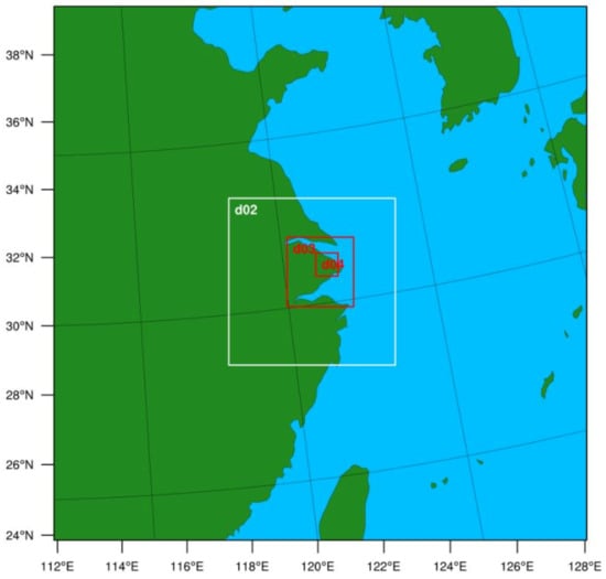
Figure 5.
Research domains in the WPS.
The output of WPS was used as inputs of ARW to process the simulation- and output-modeled meteorology. WRFv.3.4-UCM was differentiated from WRF in the ARW in a set of parameters. These parameters were designed for low residential, high residential, and commercial–industrial lands in the WRFv.3.4-UCM model in general and should be localized according to research area characteristics. The key parameters required by UCM and the values used in our model are shown in Table 2. The values for each parameter were identical for the three land uses, as cited by Zhao et al. [] and Xie et al. [].
Table 2.
Values of key parameters in the UCM models.
2.4. CMAQ Simulations of PM2.5 Pollution
A hindcast simulation was performed using the Community Multiscale Air Quality (CMAQ) model version 5.0.1. to estimate concentrations of atmospheric fine particulate matter (PM2.5) in the area surrounding Shanghai, China, during the summer, from 1–15 July 2014, and winter, from 1–15 December 2014. Model inputs included anthropogenic and biogenic emissions, meteorology, and ocean data. Anthropogenic emission inputs were prepared using the Emissions Database for Global Atmospheric Research—Hemispheric Transport of Air Pollution (EDGAR-HTAP) inventory, and biogenic emissions inputs were produced using the Model for Emissions of Gases and Aerosols from Nature (MEGAN). The outputs of these two systems were then combined prior to use by CMAQv.5.0.1. Meteorology and ocean files were obtained from the WRF models. The emission inventory is the same in both base scenario and VC scenarios. Following the completion of the simulation, evaluations were performed on both meteorological inputs and output concentrations of PM2.5 using observations from Shanghai.
2.5. Model Evaluations
Several statistical measures were calculated to evaluate the outputs of WRFv.3.4-UCM on the Shanghai base scenario on wind speed and wind direction (Equations (1)–(5)). Table 3 provides reference values to evaluate meteorology performance []. The ‘simple’ and ‘complex’ threshold values refer to the topography of the domain.
Table 3.
Results of WRF simulation evaluation and thresholds.
Root mean square error (RMSE) was calculated as the square root of the mean-squared difference in prediction-observation pairings, with valid data within a given analysis region and for a given time:
where and are the individual observed and predicted quantity at site i and time j, and the summations are over all sites (I) and time periods (T).
Mean bias error (MB) was calculated as the mean difference in prediction–observation pairings, with valid data within a given analysis region and for a given time:
Mean gross error (ME) was calculated as the mean absolute difference in prediction–observation pairings, with valid data within a given analysis region and for a given time:
The index of agreement (IOA) metric integrates all the differences between model estimates and observations within a given analysis region and for a given time period (daily) into one statistical quantity. It is the ratio of the total RMSE to the sum of two differences—between each prediction and the observed mean, and each observation and the observed mean:
where M0 is mean observation, calculated from all sites with valid data, within a given analysis region and for a given time:
Two statistical measurements were employed to evaluate the performance of PM2.5 prediction output by CMAQv.5.0.1: mean fractional bias and mean fractional error. Mean fractional bias normalized the difference (model − observed) over the sum (model + observed). A mean fractional bias of 0 indicates that the over predictions and under predictions offset each other; a positive value means that the model prediction exceeds the observation overall; a negative value means that the model prediction is under the observation overall (Equation (6)). Mean fractional error is similar to the mean fractional bias; it is expected that the absolute value of the difference is used so that the error is always positive (Equation (7)). The lower the mean fractional error is, the more accurate the prediction. R2 was also employed to measure the proportion of the variation in the observed values explained by the simulated values (Equation (8)). The mathematic expressions are shown as:
where and are the individual observed and predicted quantity at site i and time j, and the summations are over all sites (I) and time periods (T).
2.6. Assessing VCs’ Impacts on Wind Velocity and PM2.5 Concentrations
Both statistical methods and mapping visualization were employed to assess the VCs’ impacts on wind speed, wind direction, and PM2.5 concentration. Spatial–temporal assessments of PM2.5 concentration changes were comprehensively conducted to explain the VC impacts. Arc_GIS was used to visualize the meteorology map using modeling results, and Statistical Product and Service Solutions (SPSS) was employed to analyze the statistical differences among VCs.
3. Results
3.1. Evaluation Results
WRFv.3.4-UCM results showed good fitness with localized parameters in the ARW (Table 3). Wind speed predictions met the simple thresholds in both summer and winter. The RMSE was from 1.44 to 1.46 m/s. Wind direction did not meet the evaluation threshold because the observation data had certain sudden huge changes periodically. These rapid changes are usually caused by an unsteady micro-environment and could not be captured by models. Generally, WRFv.3.4-UCM can predict wind fields effectively in summer and winter in Shanghai.
The modeled PM2.5 values were calculated by summing all the pollutants of I, J, K modes of PM2.5 pollutants of CMAQv.5.0.1 outputs []. Compared to the 10 monitor observations, the mean fractional bias was −21%; the mean fractional error was 87% using hourly data. Considering the emission inventory is based on global emissions (including China), our CMAQ modeled results could be constrained and may not perfectly reflect the model performance in estimating PM2.5 concentrations. However, this could be improved after implementing local emission inventories in China in the future.
3.2. VCs Impacts on Ground Wind Velocity
The summer modeling wind speed of Shanghai is in the range of 3 to 5 m/s. The wind speed in coastal areas is higher than in the inlands (Figure 6a). Maps of the differences in wind speed among all the VC scenarios (VCs_WSPD_summer minus base_WSPD_summer) were developed. The differences in the modeling results, between −0.1 to 0.1 m/s of wind speed, are regarded as minor differences. These differences in different VC scenarios were not uniform (Figure 6b–d). The major influence of the ECO VCs exists within the northwestern corridor, and the wind speed in the ECO02 and ECO05 scenarios is slower than that in the base scenario. The major influence of the HW02 scenarios occurs in the northern lands, which are within and near the highway corridors. Lands within HW VCs have lower wind speeds, while adjacent zones to HW VCs have higher wind speeds.
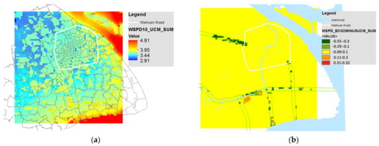
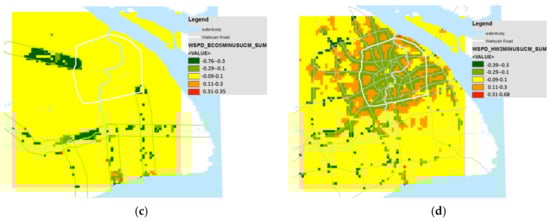
Figure 6.
(a) Modeling wind speed at 10 m high (m/s) in summer 2014; (b) modeling wind speed differences at 10 m high (m/s) in the ECO02 scenario and base scenario; (c) modeling wind speed differences at 10 m high (m/s) in the ECO05 scenario and base scenario; (d) modeling wind speed differences at 10 m high (m/s) in the HW02 scenario and base scenario.
The winter modeling wind speed of Shanghai is in the range of 3 to 7 m/s at the height of 10 m to the ground. Similar to the summer performance, coastal wind speed is higher than in the inlands (Figure 7a). Maps of PM2.5 concentration differences among all the VC scenarios and the base scenario were also constructed (VCs_windspeed_winter minus base_windspeed _winter). The differences in the modeling results, between −0.1 to 0.1 m/s of wind speed, is regarded as minor differences. The VC effects in winter are larger than in summer. The major influence of the VC scenarios is occurring in the northern lands, within and near the highway corridors (Figure 7b–d). The inside zones of VCs have lower wind speeds, while adjacent zones of VCs have higher wind speeds.
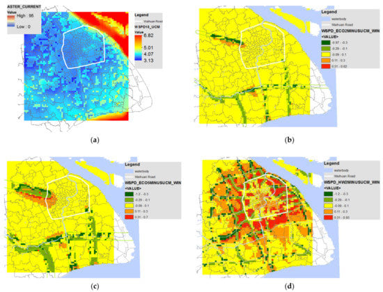
Figure 7.
(a) Modeling wind speed at 2 m high (m/s) in winter 2014; (b) modeling wind speed differences at 2 m high (m/s) in the ECO02 scenario and base scenario; (c) modeling wind speed differences at 2 m high (m/s) in the ECO05 scenario and base scenario; (d) modeling wind speed differences at 2 m high (m/s) in the HW02 scenario and base scenario.
The prevailing wind is from the southeast in the summer and from the west in the winter (Figure S1). The modeling wind directions among the base scenario and all VC scenarios were similar, based on Figure S1. It indicates that wind directions are not influenced much by the VCs in either summer or winter.
3.3. VC Impacts on PM2.5 Concentrations
The summer modeled ground-level PM2.5 of Shanghai is in the range of 2 to 45 μg/m3. The most heavily polluted areas are the west suburbs and the west city center; the coastal areas were less polluted (Figure 8a) than the inlands. Maps of the differences in PM2.5 among all the VC scenarios (VCs_PM2.5_summer minus base_PM2.5 _summer) were developed to analyze the effects of the VCs. The differences in the modeling results between −1 to +1 μg/m3 of PM2.5 concentrations are regarded as minor differences. Figure 8b–d shows that the VCs’ summer PM2.5 concentrations are higher than the baseline in the downwind areas. In the ECO_VC scenarios, certain areas have lower concentrations compared to the base scenario in the upwind of Shanghai.
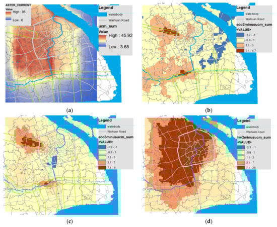
Figure 8.
(a) Modeling ground-level PM2.5 concentrations (μg/m3) in summer 2014; (b) modeling ground-level PM2.5 concentration differences (μg/m3) in the ECO02 scenario and base scenario; (c) modeling ground-level PM2.5 concentration differences (μg/m3) in the ECO05 scenario and base scenario; (d) modeling ground-level PM2.5 concentration differences (μg/m3) in the HW02 scenario and base scenario.
The winter modeled PM2.5 of Shanghai is in the range of 1 to 64 μg/m3. The most heavily polluted areas are the west suburbs and the western city center; the coastal areas are less polluted (Figure 9a). Maps of the differences in PM2.5 among all the VC scenarios (VCs_PM2.5_winter minus base_PM2.5_winter) were developed to analyze the effects of the VCs. The differences of the modeling results, between −1 to +1 μg/m3 of PM2.5 pollution concentration, are regarded as minor differences. Figure 9b–d shows that the VC scenarios’ winter PM2.5 pollution differences depend on the locations. In general, the VC-influenced areas are the VCs and adjacent areas; the affected buffer is roughly double the VCs’ width. The upwind areas (west) to the VCs show lower PM2.5 pollution concentrations, while the downwind areas (east) to the VCs have higher PM2.5 pollution concentrations than the base scenario. According to Figure 9d, the densest VC network of the HW02 scenario merely mitigates northwestern Shanghai’s PM2.5 concentrations but increases the southeastern PM2.5 concentration at the same time. The results suggest that VCs have local concentration influences in winter. The increased downwind area’s PM2.5 pollution could offset the decreasing effects when considered at the city scale.
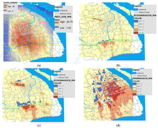
Figure 9.
(a) Modeling ground-level PM2.5 concentrations (μg/m3) in winter 2014; (b) modeling ground-level PM2.5 concentration differences (μg/m3) in the ECO02 scenario and base scenario; (c) modeling ground-level PM2.5 concentration differences (μg/m3) in the ECO05 scenario and base scenario; (d) modeling ground-level PM2.5 concentration differences (μg/m3) in the HW02 scenario and base scenario.
4. Discussion and Links to Previous Studies
The VC effects of increasing PM2.5 concentrations in certain places seem counter-intuitive but can be explained in terms of roughness change, wind field change, and pollutant transportation and deposition. Certain previous studies have been introduced to help understand our modeling results.
One of the important reasons causing the increase in PM2.5 concentration is deposition mitigation. Figure S2a,b compares the modeled base/HW02 PM2.5 dry deposition flux in summer 2014. It clearly shows that lands within the corridors in HW02 have much lower deposition flux than the base scenario. Moreover, the HW02 deposition flux decreases very sharply at night compared to the base scenario, making the original heavily polluted night period even worse (Figure 8d and Figure 9d, Table 4).
Table 4.
Time-dependent change of modeling results between the base scenario and the HW02_scenario at the Xujiahui Monitor Station and ten monitor stations from 5–15 July 2014.
Deposition flux relates to a set of parameters, such as concentrations, deposition velocity, roughness height, roughness, and boundary heights. The above factors are all modified in the VC scenarios. Equations (9) and (10) calculate the deposition flux (F) with impacting factors []:
where Vd is the deposition velocity, C is the concentration at a specific height, Ra is the aerodynamic resistance, Rb is the quasi-laminar boundary layer resistance, and Rc is the surface canopy resistance.
F = Vd × C × 3600
Despite the increase in PM2.5 concentrations, PM2.5 deposition flux still decreases by 17%, indicating sharper decreasing deposition velocity. It may be attributed to the roughness height decrease (because it weakens aerodynamic resistance (Ra)) since by applying UCM, we changed the roughness height in ventilation corridor areas for all three VC scenarios []. On top of it, by replacing previous urban land use surface categories with a grassland surface, Rb could also be changed since the convective velocity scale, w*, which is used in CMAQ to calculate Rb, has been changed. A recent study [] has added a leaf area index (LAI) in the particle dry deposition scheme in CMAQ version 5.3 to better estimate the uptake to vegetative surfaces, which could better represent the influence of changing land use categories with different VCs in this study.
Another important reason causing the increase in the VC scenarios’ PM2.5 concentrations is the planetary boundary layer (PBL) height decrease in the VC scenarios. PBL height usually shows an inverse correlation with PM2.5 concentrations []. PBL height above grasslands tends to be shorter than the height above built-up areas []. Taking the PBL differences between the medium-intensive VC scenario, ECO05, and the base scenario, for example (Figure S2c,d), the PBL heights within the VCs decrease over 15 m, and the entire Shanghai’s PBL heights also decrease in general. Further, by comparing the PBL heights in the base and the most intensive VC scenario HW02, the VC PBL heights were decreased by about 100 m in the VCs and by about −10% to −20% of the base PBL heights (Table 4) This pattern is consistent in all the VCs; thus, VCs increase PM2.5 concentrations via reducing PBL heights.
In addition, the surface ventilation velocity decrease caused by the roughness height modification also contributes to the increase in VC scenario PM2.5 concentrations. Roughness change can have two inverse effects on surface wind. On one hand, decreased roughness height weakens downward momentum transport due to less vertical mixing effects and, hence, reduces surface speeds. Second, decreased surface roughness strengthens the surface horizontal wind speeds []. By changing the heights of the existing dense buildings to grasslands in the VC scenarios, the roughness height and surface roughness are both decreased, indicating concurrent influences in surface wind speeds. According to the wind speed maps in Figure 6 and Figure 7, the vertical mixing effects seem dominant. Therefore, the wind speed within the VCs decreases and the surface PM2.5 concentration increases.
Besides the above reasons, there are references supporting the results. Barnes et al. [] developed a simpler but similar study to model NO2 concentration change before and after roughness decrease. Their model results suggest that reducing surface roughness in a city center can increase ground-level pollutant concentrations locally in both the area of reduced roughness and the downwind region. This finding is the same as this study’s. In addition, studies have also found that VCs parallel to wind directions usually have larger horizontal ventilation effects, thus decreasing pollution concentration, and VCs perpendicular to wind directions usually perform turbulent mixing effects, thus increasing pollution concentration []. Both perpendicular and parallel VCs exist in our scenarios due to land limitations, and the effects could be complicated.
5. Conclusions
In conclusion, the most economical green VCs in high-density areas such as Shanghai are grasslands or parks with sparse shrubs/trees. These VCs change PM2.5 concentrations primarily through urban-morphology-induced velocity, PBL height, and wind field modification. Although the VCs could increase ventilation speed in the nearby upwind areas to strengthen the transport of pollutants, the decrease in roughness height, deposition flux, and PBL height in or near the VCs increases local PM2.5 concentrations, and this phenomenon is more obvious in the summer.
There are several limitations to this study. First, pollution emission inventories were not modified in all the modeled scenarios, and this is not true in practice. In reality, VCs usually do not have emission sources, and their concentrations are generally lower than built-up areas. The conflicts between common reality and the modeling results suggest the VCs reduce pollution concentration by mitigating pollution sources instead of our initial assumption of strengthening dispersions. Second, the substitution of finer local emission inventories with a relatively coarse global emission inventory is an obstacle in this study. Our models need more accurate emission and pollution concentration data to improve the results in the future. Third, deposition becomes more crucial in this study since it is necessary to modify land use categories by applying different VCs; however, there still exists a gap in deposition velocity for both modeling and observation areas, making it difficult to decide the real influence of deposition velocity on our results in this study. There are several studies that have pointed out the uncertainties of particle dry deposition in air quality models [,,,]. Thus, the results of this study could be improved in the future with updated deposition algorithms. Lastly, the monitored meteorology and pollution data from different locations are also needed to verify the VC results and reasons. The conclusions do not indicate whether VCs can decrease PM2.5 pollution effectively in small cities and rural areas, at the community level, or in other materials composing the VCs. The conclusions that this study has found should be very carefully applied to other areas or scales. In the future, the model could be strengthened and validated using data from longer periods. The relationship between land use and air pollution still needs to be examined by other methods, and then the possible reasons for the differences can be cross-validated.
Supplementary Materials
The following are available online at https://www.mdpi.com/article/10.3390/atmos12101269/s1, Figure S1: (a,b) Modeling wind directions at 10m high of base, ECO02, ECO05 and HW02 scenarios in summer 2014; (c,d) Modeling wind directions at 10m height of base, ECO02, ECO05 and HW02 scenarios in winter 2014., Figure S2: (a) Modeling base PM2.5 dry deposition flux (μg/m2/h); (b) Modeling dry deposition flux (μg/m2/h) of HW02 scenario and base scenario; (c) Modeling PBL height map (meters); (d) Modeling PBL differences (meters) of ECO05 scenario and base scenario in Shanghai summer.
Author Contributions
Conceptualization, C.L.; Data curation, Q.S. and S.H.; Formal analysis, C.L.; Investigation, Q.S.; Methodology, C.L.; Writing—original draft, J.G. All authors have read and agreed to the published version of the manuscript.
Funding
This research was funded by Shanghai Natural Science Foundation, grant number 21ZR1466500.
Institutional Review Board Statement
Not applicable.
Informed Consent Statement
Not applicable.
Acknowledgments
The authors wish to acknowledge Barron H. Henderson and Zhong-ren Peng for their help in modeling development and result interpretation. This paper is funded by the Shanghai Natural Science Foundation (21ZR1466500).
Conflicts of Interest
The authors declare no conflict of interest.
References
- Huang, L.; Rao, C.; van der Kuijp, T.J.; Bi, J.; Liu, Y. A comparison of individual exposure, perception, and acceptable levels of PM2. 5 with air pollution policy objectives in China. Environ. Res. 2017, 157, 78–86. [Google Scholar] [CrossRef] [PubMed]
- Long, Y.; Wang, J.; Wu, K.; Zhang, J. Population exposure to ambient PM2. 5 at the subdistrict level in China. Int. J. Environ. Res. Public Health 2018, 15, 2683. [Google Scholar] [CrossRef] [PubMed] [Green Version]
- Ren, C.; Yuan, C.; Ho, C.K.; NG, Y.Y. A study of air path and its application in urban planning. Urban Plan. Forum 2014, 3, 52–60. [Google Scholar]
- Kastner-Klein, P.; Plate, E. Wind-tunnel study of concentration fields in street canyons. Atmos. Environ. 1999, 33, 3973–3979. [Google Scholar] [CrossRef]
- Taseiko, O.V.; Mikhailuta, S.V.; Pitt, A.; Lezhenin, A.A.; Zakharov, Y.V. Air pollution dispersion within urban street canyons. Atmos. Environ. 2009, 43, 245–252. [Google Scholar] [CrossRef]
- Yuan, C.; Ng, E.; Norford, L.K. Improving air quality in high-density cities by understanding the relationship between air pollutant dispersion and urban morphologies. Build. Environ. 2014, 71, 245–258. [Google Scholar] [CrossRef]
- Yu, K.; Zhang, L.; Yanng, Z.; Wang, X.; Liu, M. Eco-city Construction. In Contemporary Ecology Research in China; Springer: Berlin/Heidelberg, Germany, 2015; pp. 555–624. [Google Scholar]
- Tominaga, Y.; Stathopoulos, T. CFD simulation of near-field pollutant dispersion in the urban environment: A review of current modeling techniques. Atmos. Environ. 2013, 79, 716–730. [Google Scholar] [CrossRef] [Green Version]
- Papangelis, G.; Tombrou, M.; Dandou, A.; Kontos, T. An urban “green planning” approach utilizing the Weather Research and Forecasting (WRF) modeling system. A case study of Athens, Greece. Landsc. Urban Plan. 2012, 105, 174–183. [Google Scholar] [CrossRef]
- Pearce, J.L.; Beringer, J.; Nicholls, N.; Hyndman, R.J.; Tapper, N.J. Quantifying the influence of local meteorology on air quality using generalized additive models. Atmos. Environ. 2011, 45, 1328–1336. [Google Scholar] [CrossRef]
- Weng, Q.; Yang, S. Urban air pollution patterns, land use, and thermal landscape: An examination of the linkage using GIS. Environ. Monit. Assess. 2006, 117, 463–489. [Google Scholar] [CrossRef]
- Jerrett, M.; Arain, A.; Kanaroglou, P.; Beckerman, B.; Potoglou, D.; Sahsuvaroglu, T.; Morrison, J.; Giovis, C. A review and evaluation of intraurban air pollution exposure models. J. Expo. Sci. Environ. Epidemiol. 2005, 15, 185–204. [Google Scholar] [CrossRef]
- Barnes, M.; Brade, T.K.; Mackenzie, A.R.; Whyatt, J.; Carruthers, D.; Stocker, J.; Cai, X.; Hewitt, C. Spatially-varying surface roughness and ground-level air quality in an operational dispersion model. Environ. Pollut. 2014, 185, 44–51. [Google Scholar] [CrossRef]
- Chen, F.; Kusaka, H.; Bornstein, R.; Ching, J.; Grimmond, C.; Grossman-Clarke, S.; Loridan, T.; Manning, K.W.; Martilli, A.; Miao, S. The integrated WRF/urban modelling system: Development, evaluation, and applications to urban environmental problems. Int. J. Climatol. 2011, 31, 273–288. [Google Scholar] [CrossRef]
- Tewari, M.; Chen, F.; Kusaka, H. Implementation and Evaluation of a Single-Layer Urban Canopy Model in WRF/Noah. Available online: https://citeseerx.ist.psu.edu/viewdoc/download?doi=10.1.1.470.716&rep=rep1&type=pdf (accessed on 22 September 2021).
- Chen, F.; Kusaka, H.; Tewari, M.; Bao, J.; Hirakuchi, H. Utilizing the coupled WRF/LSM/Urban modeling system with detailed urban classification to simulate the urban heat island phenomena over the Greater Houston area. In Proceedings of the Fifth Symposium on the Urban Environment, Vancouver, BC, Canada, 23 August 2004; pp. 9–11. [Google Scholar]
- Lin, C.-Y.; Su, C.-J.; Kusaka, H.; Akimoto, Y.; Sheng, Y.-F.; Huang, J.-C.; Hsu, H.-H. Impact of an improved WRF urban canopy model on diurnal air temperature simulation over northern Taiwan. Atmos. Chem. Phys. 2016, 16, 1809–1822. [Google Scholar] [CrossRef] [Green Version]
- Ching, J.; Byun, D. Introduction to the Models-3 Framework and the Community Multiscale Air Quality Model (CMAQ). Available online: https://www.cmascenter.org/cmaq/science_documentation/pdf/ch01.pdf (accessed on 22 September 2021).
- Koo, Y.-S.; Kim, S.-T.; Yun, H.-Y.; Han, J.-S.; Lee, J.-Y.; Kim, K.-H.; Jeon, E.-C. The simulation of aerosol transport over East Asia region. Atmos. Res. 2008, 90, 264–271. [Google Scholar] [CrossRef]
- Marshall, J.D.; Nethery, E.; Brauer, M. Within-urban variability in ambient air pollution: Comparison of estimation methods. Atmos. Environ. 2008, 42, 1359–1369. [Google Scholar] [CrossRef]
- Nolte, C.; Appel, K.; Kelly, J.; Bhave, P.; Fahey, K.; Collett, J., Jr.; Zhang, L.; Young, J. Evaluation of the Community Multiscale Air Quality (CMAQ) model v5. 0 against size-resolved measurements of inorganic particle composition across sites in North America. Geosci. Model Dev. 2015, 8, 2877–2892. [Google Scholar] [CrossRef] [Green Version]
- Briggs, D.J.; Collins, S.; Elliott, P.; Fischer, P.; Kingham, S.; Lebret, E.; Pryl, K.; Van Reeuwijk, H.; Smallbone, K.; Van Der Veen, A. Mapping urban air pollution using GIS: A regression-based approach. Int. J. Geogr. Inf. Sci. 1997, 11, 699–718. [Google Scholar] [CrossRef] [Green Version]
- Liu, C.; Henderson, B.H.; Wang, D.; Yang, X.; Peng, Z.-r. A land use regression application into assessing spatial variation of intra-urban fine particulate matter (PM2. 5) and nitrogen dioxide (NO2) concentrations in City of Shanghai, China. Sci. Total Environ. 2016, 565, 607–615. [Google Scholar] [CrossRef]
- Gallagher, J.; Baldauf, R.; Fuller, C.H.; Kumar, P.; Gill, L.W.; McNabola, A. Passive methods for improving air quality in the built environment: A review of porous and solid barriers. Atmos. Environ. 2015, 120, 61–70. [Google Scholar] [CrossRef]
- SHGTJ. Shanghai Ecological Protective Plan. Available online: https://ghzyj.sh.gov.cn/ghgs/20200415/0032-965690.html (accessed on 14 April 2021).
- Zhao, W.; Zhang, N.; Sun, J.; Zou, J. Evaluation and parameter-sensitivity study of a single-layer urban canopy model (SLUCM) with measurements in Nanjing, China. J. Hydrometeorol. 2014, 15, 1078–1090. [Google Scholar] [CrossRef]
- Xie, M.; Liao, J.; Wang, T.; Zhu, K.; Zhuang, B.; Han, Y.; Li, M.; Li, S. Modeling of the anthropogenic heat flux and its effect on regional meteorology and air quality over the Yangtze River Delta region, China. Atmos. Chem. Phys. 2016, 16, 6071–6089. [Google Scholar] [CrossRef] [Green Version]
- Emery, C.; Tai, E.; Yarwood, G. Enhanced Meteorological Modeling and Performance Evaluation for Two Texas Ozone Episodes. Available online: https://www.semanticscholar.org/paper/Enhanced-Meteorological-Modeling-and-Performance-Emery-Tai/3faa521b77acb7158769d9523be8f33e1d7e7ec6 (accessed on 22 September 2021).
- Wesely, M.; Hicks, B. Some factors that affect the deposition rates of sulfur dioxide and similar gases on vegetation. J. Air Pollut. Control Assoc. 1977, 27, 1110–1116. [Google Scholar] [CrossRef] [Green Version]
- Matsuda, K.; Fukuzaki, N.; Maeda, M. A case study on estimation of dry deposition of sulfur and nitrogen compounds by inferential method. Water Air Soil Pollut. 2001, 130, 553–558. [Google Scholar] [CrossRef]
- Shu, Q.; Murphy, B.; Pleim, J.E.; Schwede, D.; Henderson, B.H.; Pye, H.O.; Appel, K.W.; Khan, T.R.; Perlinger, J.A. Particle dry deposition algorithms in CMAQ version 5.3: Characterization of critical parameters and land use dependence using DepoBoxTool version 1.0. Geosci. Model Dev. Discuss. 2021, 1–29. [Google Scholar] [CrossRef]
- Liu, Y.; Paciorek, C.J.; Koutrakis, P. Estimating regional spatial and temporal variability of PM2. 5 concentrations using satellite data, meteorology, and land use information. Environ. Health Perspect. 2009, 117, 886–892. [Google Scholar] [CrossRef] [Green Version]
- Lee, S.-H.; Kim, S.-W.; Angevine, W.; Bianco, L.; McKeen, S.; Senff, C.; Trainer, M.; Tucker, S.; Zamora, R. Evaluation of urban surface parameterizations in the WRF model using measurements during the Texas Air Quality Study 2006 field campaign. Atmos. Chem. Phys. 2011, 11, 2127–2143. [Google Scholar] [CrossRef] [Green Version]
- Kamal, S.; Huang, H.-P.; Myint, S.W. The influence of urbanization on the climate of the Las Vegas metropolitan area: A numerical study. J. Appl. Meteorol. Climatol. 2015, 54, 2157–2177. [Google Scholar] [CrossRef]
- Shu, Q.; Koo, B.; Yarwood, G.; Henderson, B.H. Strong influence of deposition and vertical mixing on secondary organic aerosol concentrations in CMAQ and CAMx. Atmos. Environ. 2017, 171, 317–329. [Google Scholar] [CrossRef]
- Saylor, R.D.; Baker, B.D.; Lee, P.; Tong, D.; Pan, L.; Hicks, B.B. The particle dry deposition component of total deposition from air quality models: Right, wrong or uncertain? Tellus B Chem. Phys. Meteorol. 2019, 71, 1550324. [Google Scholar] [CrossRef] [Green Version]
- Emerson, E.W.; Hodshire, A.L.; DeBolt, H.M.; Bilsback, K.R.; Pierce, J.R.; McMeeking, G.R.; Farmer, D.K. Revisiting particle dry deposition and its role in radiative effect estimates. Proc. Natl. Acad. Sci. USA 2020, 117, 26076–26082. [Google Scholar] [CrossRef] [PubMed]
Publisher’s Note: MDPI stays neutral with regard to jurisdictional claims in published maps and institutional affiliations. |
© 2021 by the authors. Licensee MDPI, Basel, Switzerland. This article is an open access article distributed under the terms and conditions of the Creative Commons Attribution (CC BY) license (https://creativecommons.org/licenses/by/4.0/).