Article

Optimization of HPC Use for 3D High Resolution Urban Air Quality Assessment and Downstream Services

1
ARIA Technologies, 92100 Boulogne-Billancourt, France
2
ARIANET S.R.L., 20128 Milan, Italy
*
Author to whom correspondence should be addressed.
Atmosphere 2021, 12(11), 1410; https://doi.org/10.3390/atmos12111410
Submission received: 22 September 2021 / Revised: 21 October 2021 / Accepted: 22 October 2021 / Published: 26 October 2021

Abstract

:
The number of cities, or parts of cities, where air quality has been computed using the PMSS 3D model now appears to be sufficient to allow assessment and understanding of performance. Two fields of application explain the growing number of sites: the first is the long-term air quality assessment required in urban areas for any building or road project. The geometric complexity found in such areas can justify the use of a 3D approach, as opposed to Gaussian ones. However, these studies have constraining rules that can make the modelling challenging: several scenarios are needed (current, future with project, future without project), the long-term impact implies a long physical time period to be computed, and the spatial extension of the domain can be large in order to cover the traffic impact zone of the project. The second type of application is dedicated to services and, essentially, to forecasting. As for impact assessments, the modelling can be challenging here because of the extension of the domain if the target area is a whole city. Forecast also adds the constraint of time, as results are requested early, and the constraint of robustness. The CPU amount needed to meet all these requirements is important. It is therefore crucial to optimize all possible parts of the modelling chain in order to limit cost and delay. The sites presented in the article have been modelled with PMSS for long periods. This allows feedback to be provided on different topics: (a) daily forecasts offer an opportunity to increase the robustness of the modelling chain; (b) quantitative validation at air quality measurement stations; (c) comparison of annual impact based on a whole year, and based on a sampling list of dates selected thanks to a classification process; (d) large calculation domains with widespread pollutant emissions offer a great opportunity to qualitatively check and improve model results on numerous geometrical configurations; (e) CPU time variations between different sites provide valuable information to select the best parametrizations, to predict the cost of the services, and to design the needed hardware for a new site.

1. Introduction

1.1. General Context and Motivations

Air pollution is known to impact health strongly: the World Health Organization estimates today that it kills approximatively 7 million people per year. Exposure is especially alarming in dense urban areas, where both population and pollutant emissions are high.
Methodologies for estimating the exposure in cities is therefore fundamental to describe current and future situations, and define improvement strategies.
Air quality in cities results not only from local emissions, but is a complex system that can be described by the following simplifications [1]: the regional-scale contribution which have a uniform impact on the city; the city-scale contribution, including emissions from heating for example, that is uniformly considered within the city or within the different districts of the city according to the spatial resolution of the available emission inventory; and the street-scale contribution, which are related mainly to local traffic emissions, and are highly non-uniform.
The present article is focused on the deterministic modelling of the street-scale contribution. As air quality observations provide concentration measurements of all the contributions, model validation is not performed with only the street-scale, but also with the larger scale contributions that can be named “background contribution”.
Modeling provides additional and complementary information to air quality monitoring networks that are limited to a given number of measurement points: exposure maps detailing spatial gradients are one of the added values of modeling. Urban micro-meteorology has been studied since the 1980s [2], and different types of approaches, ranging from simple analytical formulations (Gaussian models) to full fluid dynamics (CFD models), are used nowadays [3].
The approach is noticeably chosen depending on the objectives, the time, and budget constraints. The present article deals with applications where both 3D high resolution and limited CPU time are required, and for which the PMSS modeling system is an applied solution.

1.2. The PMSS Modeling System

Parallel-Micro-SWIFT-SPRAY (PMSS) is a flow and dispersion modelling system constituted by the SWIFT and SPRAY models. They became Micro-SWIFT and Micro-SPRAY when explicit consideration of the obstacles [4,5] was added based on the preliminary work of Rockle [6], with the principal objective of rapid modelling (faster than a full CFD model) of the accidental or malicious dispersion of pollutants in dense urban areas. PMSS has then been improved, and parallel versions of Micro-SWIFT and Micro-SPRAY (abbreviated as PSWIFT and PSPRAY) have been developed [7,8]. Recent validations in this scope of application are presented in [9,10].
The rapid nature of PMSS and the increase in power of the computational machines then enabled, in addition to the defense-oriented use, the study of air quality in dense urban areas, often highly impacted by road traffic. The model was first used on neighborhoods such as Bologna [5], and then on entire cities such as Paris [11]. In this type of application, the number of sources to be considered is much more important, and makes the calculation more CPU expensive.
PSWIFT [1] is a 3D diagnostic, mass-consistent, terrain-following model providing the wind, turbulence, and temperature following three main steps:
  • A first guess computation based on the interpolation of heterogeneous meteorological input data, a mix of surface and profile measurements, and/or possibly meso-scale model outputs;
  • The modification of the first guess using analytical zones defined around isolated buildings or within groups of buildings, based the approach originally proposed by [6];
  • The mass-consistency (with impermeability condition at the ground and buildings) obtained by minimizing the difference of the wind field of the second step over the volume of the domain under the mass conservation constraint. The effect of atmospheric stability on the flow around obstacles is considered through a coefficient α applied to the vertical wind component terms during the minimizing process [12].
The method allows detailed flow fields in the urban environment to be generated within a matter of minutes [13]. To consider traffic-produced turbulence (TPT) in street canyons, a formulation based on the OSPM model [14] has been added, increasing the turbulent kinetic energy field predicted by PSWIFT in these zones according to vehicles fluxes, speed, and effective area.
PSPRAY is a 3D Lagrangian particle dispersion model (LPDM) [15], directly derived from the SPRAY code [16,17,18,19,20,21,22]. The dispersion of a pollutant (gas or fine aerosol) is simulated following the trajectories of a large number of numerical particles. The trajectories are obtained by integrating in time the particle velocity, which is the sum of a transport component defined by the local averaged wind provided by PSWIFT, and a stochastic component representing the dispersion due to the atmospheric turbulence. The stochastic component is obtained by solving a 3D form of the Langevin equation for the random velocity, and applying the stochastic scheme developed by Thomson [23].
To consider the transformation between NO and NO2, a simple chemical scheme has been added in PSPRAY [24].

1.3. The Different Type of High Resolution Air Quality Modeling Applications

In France, the two main frameworks in which such modelling are used are regulatory impact studies for road or building projects, and forecasting (or now-casting) systems operated by territorial agencies. The number of neighborhoods or cities modelled in these contexts with PMSS now seems to be sufficiently large to gather different feedbacks and optimization methods of the computational resource in the present article, with the goal of satisfying temporal and budgetary constraints.
In the first section, different reasons making the use of HPC useful for long-term impact studies of air quality in cities are presented. In some examples, optimization methods of computing resources and modelling validations are also presented. It should be noted that for most impact studies, contractual context frequently does not allow for the publication of results. These studies, limited in terms of budget, also don’t include modelling validation. Consequently, in this article, only the results obtained in the study of chronic pollution in the framework of collaborative research and innovation projects are presented.
In the second section, feedback is presented from forecasting systems incorporating the PMSS model. This type of system poses a significant performance constraint in terms of computational time in order to obtain results early enough.
Finally, the third section gathers information on the configuration parameters of the model, on the computational machines used, and on the performances obtained, in order to identify useful trends for specifying the resources required for future modelling of the same type.

2. Long Term Air Quality Assessment in Urban Areas

2.1. Why Is HPC Used?

In France, urban development projects can be subjected to environmental assessment or to a case-by-case analysis according to criteria and thresholds (decree No. 2020-844 of 3 July 2020 on the environmental authority and the authority responsible for the examination of the case). The content of the “air and health” section of impact studies is defined in the methodological guide provided with the technical note of “22 February 2019”, related to consideration of the health effects of air pollution in road infrastructure impact studies. According to this methodological guide, air concentrations that are induced by the project must be estimated with the help of a dispersion model.
Several specificities of these development project impact studies on air quality in dense urban areas potentially lead to a model choice whose complexity and computational cost guide towards the use of HPC machines. The following section describes these different specificities, partially within the prism of French regulations.

2.1.1. Complex Geometry

The first element is the geometric context of this type of study: in a dense urban area, the volume occupied by buildings is important. Inside Paris, for example, 39% of land is covered with buildings (calculated from the BD TOPO database of the National Geographic Institute (IGN)). This significant percentage implies a calculation error of the pollutant concentration for modelling approaches that do not consider the volume occupied by buildings. This is the case, for example, for Gaussian models such as CALINE4 [25], for which concentration underestimations are recorded by [26] for a canyon street configuration. The operational street pollution model, OSPM [27], takes into account the confinement effect in street canyons, while keeping an inexpensive approach in terms of computation time.
The high buildings density and their organization into streets, crossroads, and blocks of houses also involve channeling effects. The Gaussian approach to model the dispersion can then be upgraded, as in the SIRANE model [28], with pollutant mass exchange algorithms both at the top of canyon streets, and at crossroads between road segments. Modelling consequently remains inexpensive in terms of computing time.
These approaches are based on the geometric hypothesis of a classic or semi-open canyon street with a uniform building height along the street. To address any geometric configurations, it seems required to explicitly take into consideration the volumes of each building, for example, by constructing an unstructured mesh around it, or by projecting these volumes on a structured mesh. This spatial discretization is typical for CFD models, which are, however, more expensive in terms of computation time. In the atmospheric dispersion field, the family of models based on Rockle’s work [6], such as PSWIFT, provides less expensive alternatives compared to full CFD models [29].

2.1.2. Unsteady Meteorology and Unsteady Emissions

A second specificity of impact studies is the temporal variability, both in terms of meteorological conditions, and pollutant emissions. This double variability raises questions concerning the use of steady or unsteady models, and increases the potential number of situations to be modelled.

Steady versus Unsteady Approaches

Straight-lined Gaussian models are stationary by construction, and the most complete models, such as the CFD models, can also be used in a stationary way within the atmospheric dispersion framework when the considered meteorological conditions and emissions are constants. To calculate an annual impact, a number (often limited for the more expensive models) of these steady-state situations is simulated, and an average, weighted by the frequency of occurrence of each situation, is used to estimate annual values. This approach was used in 2020, for example, on the impact study of the developing project around the Eiffel Tower (https://www.paris.fr/pages/grand-site-tour-eiffel-un-poumon-vert-au-c-ur-de-paris-6810/ (accessed on 10 September 2021)), and for the developing project at the “Porte de Montreuil” (https://www.paris.fr/pages/20-e-porte-de-montreuil-3329 (accessed on 10 September 2021)). It can be described as a frequency approach. The transitory aspect of the dispersion is neglected. To take it into account, it is necessary to use an unsteady dispersion model over sequences of several hours or several days for example, and ideally, over a full year. Today, calculating sequences over several days with a full CFD model seems to be too costly, in terms of computation time, to be compatible with deadlines and the total costs of impact studies, however, with intermediate approaches such as PMSS, it is reasonable, and already done for many studies. A complete one-year sequence is a possible approach (sequential approach), but in practice, the selection of a few dozen typical days (several 24 h sequences) is more affordable. The latter has been used, for example, in the impact study of the Porte Maillot project in 2019 (https://www.paris.fr/pages/projet-16e-17e-porte-maillot-4559 (accessed on 10 September 2021)). It is then both a sequential and frequential approach. This trade-off is detailed in a concrete study case in Section 2.2.

Input Data Cross-Variability

Time variability in meteorology and emissions implies, for a frequential approach, choosing the most representative combinations, a task which might not be trivial. For example, if low winds are rather nocturnal and, therefore, associated with low traffic periods, in winter, the night can last until the morning peak traffic. The situation then penalizes the air quality because of weak winds and large emissions, and might be considered in the selection. However, in a frequential approach, the limited number of cases often entails the impossibility of considering this type of specific combination because only average daily traffic values are used.

2.1.3. Purifying Systems

In order to bring a contribution to the air quality improvement in cities, some development projects include depollution systems. The use of a high-level model with a sufficient complexity is required in order to take into account the effects of the depollution systems, and quantify the extent of the affected zone in three dimensions.

2.1.4. Numerous Scenarios

In France, the methodological guide, coming with the technological note of “22 February 2019”, related to the effects of air pollution on health in impact studies of road infrastructures, states the necessity of examining numerous scenarios: the current situation, and the future situation at different horizons (at least at the commissioning of the project, and up to 20 years after the commissioning, with and without the project)—at least five scenarios for each project should be examined. As deadlines to conduct impact studies are often short, it is necessary to use powerful computing machines to complete all of the calculations.

2.1.5. Domain Extents

For road development impact studies, French regulations require the computational domain to cover the zone for which road traffic is modified by 10%. Areas that must be modelled can then be far more extended than the development project itself. As an example, for the development of the Eiffel Tower neighborhood (Autorité Environnementale, 2020 Avis délibéré de l’Autorité environnementale sur l’aménagement du site de la Tour Eiffel (75)—N° Ae 2020-115), the project’s extension is included in a 1.5 km × 1.5 km area, and the computation domain for the modelling of the air quality is 7 km × 5.3 km.

2.2. Annual Impact on a Coastal City with Very Complex Terrain—HPC Use Optimization with Classification

2.2.1. Presentation and Objectives

The computation times of PMSS can lead to costly annual impact studies of a site when many sources are being considered. As discussed in the previous section, for an urban site with emissions linked to road traffic, a classification of the input data (meteorological data for example), allows for the selection of a few entire days to model. Statistics, and, in particular, average concentrations, are therefore calculated from a few dozen days, but not from the whole year. The use of classified input data allows the computation time to be restricted, while keeping the benefits associated with the modelling of continuous sequences, taking into account diurnal cycle and emission modulations.
Self-organized maps (SOMs) is the classification method used in the study presented in this section. It is based on artificial neural networks that operate through unsupervised learning [30]. This method was introduced in the context of atmospheric studies in the late 1990s as a classification and shape recognition method. The article [31] reviews the applications of the SOMs method to meteorology and oceanography. This method is shown to be useful at very different spatial and temporal scales. The current study proposes verifying that the SOMs classification of the input data allows for the estimation of a yearly average and percentiles of concentrations close to those obtained without SOMs classification. Percentiles are important to assess the frequencies of exceedances for regulatory impact studies. Estimating these values with the classification is more challenging than annual averages because classifications tend to approximate statistical tails less accurately.
This study, in collaboration with Atmo Sud, deals with the air quality modelling of a port agglomeration in the south of France. The horizontal extent of the study domain is about 3.6 km by 4.6 km. Given the street types of the agglomeration, a 3 m resolution was chosen for the whole domain to efficiently model the dispersion of the pollutant in the urban fabric. The steep topography culminates at 770 m. The 3D buildings database (BD TOPO IGN) has 3637 polygons in the modelled domain. The road network is described in 1382 sections, on average 101 m long, but whose length can vary from a few meters up to 3.3 km. Hourly meteorological data from a station located in the computation domain is integrated as an input to the PMSS model. Pollutant emissions from road traffic were modelled with the COPERT 5 method, and were provided by Atmo Sud with time modulation profiles for business days, Saturdays, Sundays, and holidays. Atmo Sud also provided the emissions from an incinerator located in the modelled domain with the thermodynamic properties of the chimneys (height, temperature, expulsion speed of the discharges at the chimney output). Other sources of pollutants are taken into account by integrating background concentrations recorded at urban background stations located in the modelled area. These stations are supposed to be located outside of the direct influence of the sources that are explicitly modelled.
NO2 concentrations are herewith presented. PM10 and PM2.5 concentrations have also been analyzed. As the conclusions from the SOMs classification assessment are similar, they are not presented. Background concentrations of NO2 were recorded at two measurement stations, but only the minimum value is selected as the background concentration. O3 background was also extracted from observations at background monitoring stations.

2.2.2. Model Performance without Classification

Days without observations were not modelled. Consequently, the year 2017 counted 359 days that could be modelled. In this first part of the study, all the available days were considered. Calculations were carried out at the CALMIP computation center (University of Toulouse). With PSWIFT, one day is modelled in 15 min by allocating 151 computation cores, whereas PSPRAY runs for 91 min with 240 computation cores. In comparison with a Eulerian model such as PSWIFT, the Lagrangian approach of the PSPRAY model implies a significant variability of the computation time, mainly according to meteorological situation. For example, the 15 March was modelled in 102 min, whereas the 17 March was modelled in 76 min.
In the context of the project, in 2018, Atmo Sud conducted a measurement campaign to complete the field diagnostic by bringing complementary data to the five permanent stations located in the modelled area.
Table 1 presents the scores obtained for hourly concentrations at the five stations. The high scores at station three can be explained by the fact that the values at this station were used as input data for the model.
In addition to the five permanent stations, passive NO2 measuring samplers were positioned on 37 locations in the modelled domain. The locations of the measurements aim to better characterize air quality at a fine scale on the modelled area. Particular attention has been paid to consider:
  • Different neighborhoods, in order to evaluate the distribution of the concentrations, and to better consider the impact of the topography;
  • Major road axes crossing the territory, and those with a canyon-type;
  • The acquisition of measurements in the vicinity of atypical sources of emissions (proximity to heliports, gas stations, cruise ships quays, tunnel portals, etc.).
Sampling took place over two periods of the year. The first took place during the winter between the 22 January and the 26 February, whereas the second one took place between the 19 June and the 17 July in the summer season. Assessing two distinct periods allows for the inclusion of seasonal meteorological variations, as well as activity variations on the territory. Linear regression coefficients to estimate the 2017 annual average as a function of the values obtained during the campaign (average of summer and winter) were established for the permanent stations. These linear regression coefficients are then used to estimate average concentrations for 2017 of each passive sample.
Figure 1a shows the average observed concentrations for 2017 at the passive samplers for NO2, and those computed with the PMSS model. The figure shows a significant heterogeneity in concentration levels, and this observation is generally valid for dense urban centers. For 86% of the points in Figure 1a, a vast majority of them, the PMSS model is less than 10 µg·m−3 from the observations. The regression line shows a slight underestimation of PMSS. The origin of this underestimation is difficult to isolate, and probably results from the different intermediate approximations. Figure 1b shows the annual average and 99.8th percentile estimated by PMSS at the five permanent stations. The calculation of the annual average also presents a slight underestimation. In the case of three stations out of five, an underestimation is observed by the model for the 99.8th percentile. The line «y = x/2» shows, however, that these values remain within a factor of 2 of the observations.

2.2.3. Results with SOMs Classification

All the elements that need to be classified (vectors) at the input of SOMs are of the same size: there are 359 days (vectors) described in hourly step, and each component of these vectors can be the 24 values of speed, and (or) of direction, and of temperature, etc. The SOMs classification is applied to two sets of surface data from permanent monitoring stations. In the c1 setup, the input data of SOMs are wind speed, its direction, humidity, and temperature, whereas setup c2 also includes background concentrations (PM10, PM25, NO, NO2, O3).
Input data processing is applied before the SOMs classification. The comparison between vectors is based on a Euclidian distance. In order to not privilege components with high values (temperatures in Kelvin for example) over those with low values (wind amplitudes in m·s−1 for example), the variables were standardized (zero mean and standard deviation of 1). The wind direction and its magnitude are preferred to wind components, in order to preserve the angle notion in the classification. This was not the case in this example, however, a shift of 90° might be considered if the north sector is a dominant direction of the wind (because of the proximity between 359° and 1°).
One of the parameters of the SOMs classification algorithm is the targeted class number Nc, defined as the product of two integers Nc = Xdim.Ydim. The SOMs method forms a grid with Xdim.Ydim nodes, where each node is associated with a vector. The classification is done through two successive learning phases, where the second one is finer than the first one. In this study, the number of neighbors of a node is fixed at 4 (rectangular grid), and all the nodes are modified by each input vector, with a respective weight that decreases with distance. Three-hundred fifty-nine vectors at the input are divided into Nc classes. A Euclidian distance between vectors and the barycenter of “their class” is calculated, and the vector with the smallest distance is acknowledged as the best representative of the class. The modelling of this day (=vector) with PMSS thus represents its class. It is then necessary to choose a method to rebuild a complete time history, in order to compute annual means and percentiles from the Nc best representatives modelled with PMSS. Two reconstruction methods are tested: an unmodelled day is represented by “its best” representative among those modelled (method m1); or by a weighted sum of the modelled days (method m2), with a weighting chosen from the Euclidean distance between a representative and the studied day (the weighting is described in [32]).
The symmetry of the SOMs classification has been checked. This means that a classification with Nc = Xdim.Ydim classes is identical to the classification with the Ydim.Xdim classes. It must, however, be noted that a number of classes can be obtained in several ways (40 = 5 × 8 = 4 × 10), and as many different classifications. For this study, and for the convergence analysis, the number of targeted classes is chosen as 5 × 5 = 25 and 10 × 10 = 100. Concentrations are extracted from the five air quality monitoring stations located in the calculation domain. Table 2 summarizes the presented elements.
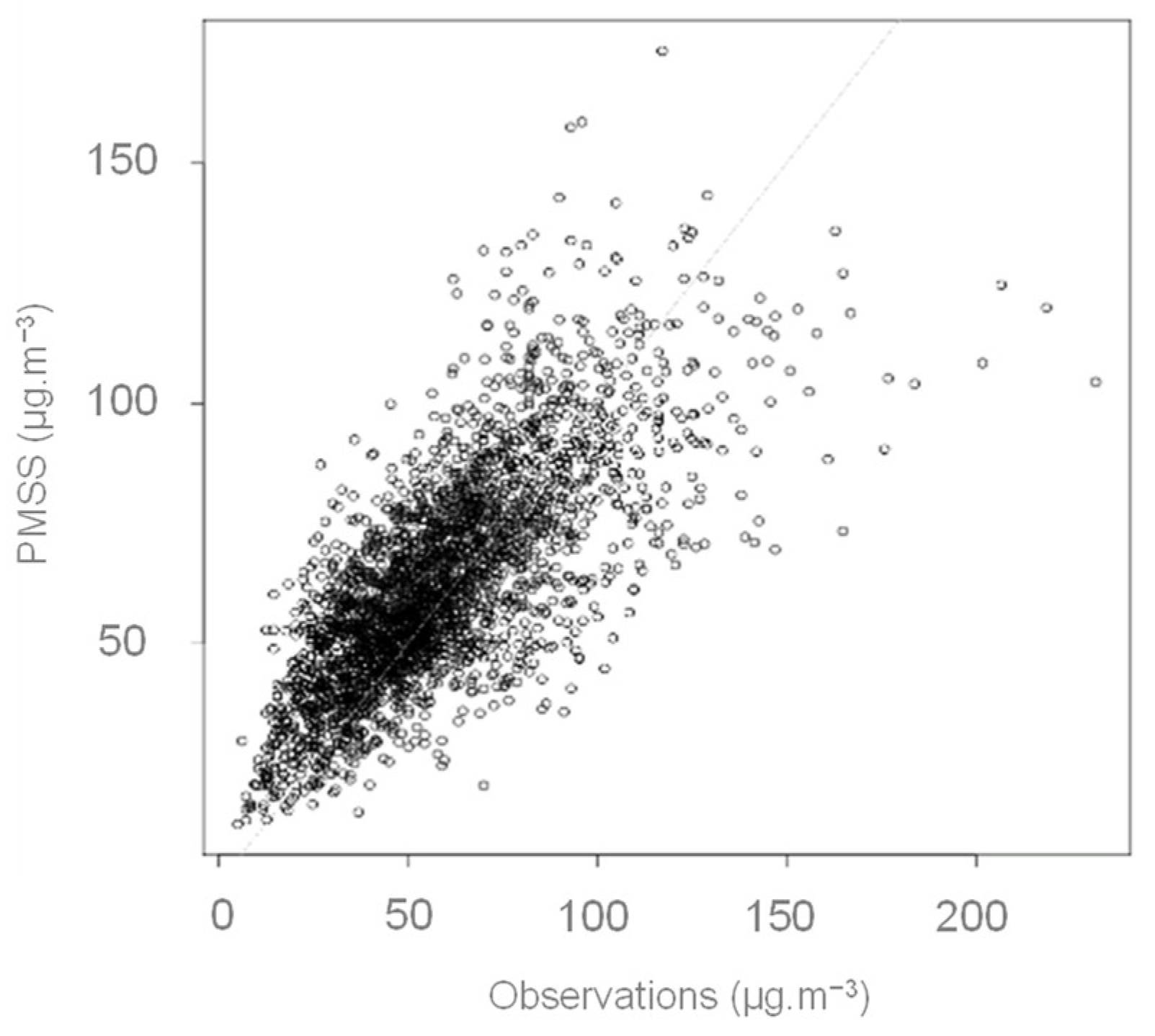
For the eight possible cross configurations (setup/reconstruction/Nc), Figure 2 shows the obtained values for the annual mean estimate (left) and the 95th percentile (right). Other statistics, such as the median and the 5th percentile, were also analyzed, and present similar conclusions. The regression lines allow an aggregation of the values at the five stations, and the correlation coefficients R2 of the different lines are all superior to 0.995.
A greater gap with and without the classification is observed on the 95th percentile than on averages. A greater deviation also implies that the regression line moves away from the perfect correlation (y = x). The classification tends to underestimate the means and the 95th percentile values, and tends to overestimate the 5th percentiles. This is consistent with the complexity for the classifications to properly reproduce statistical distribution tails. However, errors remain in the order of 5 µg·m−3, and are less than 2 µg·m−3 for the means. The consideration of the background concentrations (setup c2) substantially improves the means and the 95th percentile values estimation. It is consistent with the fact that air quality in urban areas is not only sensitive to local emissions, but also to background concentrations, with air quality being a multiscale issue. The 95th percentile estimate with the c1 setup does not seem to depend on the number of classes. In other cases, a decrease in the differences is observed overall with the increase of the number of classes. For the percentile’s estimation in the c2 setup, this decrease is actually faster for the reconstruction method m1. This last finding is understandable because method 2 (m2) represents the unmodelled days by a weighted sum of all the representatives, and thus, smooths the complete time history more than the m1 method does. Annual means do not seem responsive to the reconstruction model, and this also remains true for each annual means at a specific hour (not shown here).

2.3. Grenoble Case—Validation with High Density Sensors Network

2.3.1. Context and Model Setup

A modelling at the local scale is operated on the Grenoble agglomeration by Atmo Auvergne Rhône Alpes (Atmo AURA), mainly based on the SIRANE model. In 2016–2018, the Mobicit’air project has also allowed the evaluation of different methodologies for the assimilation of concentration observations (https://www.atmo-auvergnerhonealpes.fr/sites/ra/files/atoms/files/rapport_final_mobicitair_lot3.pdf (accessed on 10 September 2021), published in 2017) with a relatively high density of sensors, thanks to the use of micro-sensors, which are less costly than reference stations with analyzers. In 2018–2019, as part of the FUI FAIRCITY project (https://www.axelera.org/fr/actualite/Projet-Faircity (accessed on 10 September 2021), published in 2019), this measurement campaign, including micro-sensors and reference stations, was used to assess the performance of the PMSS model, and develop a coupling methodology between SIRANE and PMSS. The coupling, which is not detailed in this article, aims to allow the application of PMSS on a sub-domain to the one of SIRANE. It is based on the creation of groups of emission sources in the SIRANE input in order to be able to access the effects of all sources, but also of all sources except the ones taken into account by PMSS. This specification in the larger scale modelling (here SIRANE) allows for the summing of the concentrations of PMSS and SIRANE in the PMSS subdomain without double counting. This summation assumes a linearity of the sources’ contributions particularly, despite chemical reactions in the atmosphere, such as NO/NO2 conversion.
The PMSS computation domain is 1770 m × 1671 m, located in the center of Grenoble (the SIRANE domain extent is, in comparison, 32 km × 44 km). The horizontal spatial resolution is 3 m. The vertical spatial resolution is 2 m between the ground and the first 10 m, then progressively decreases up to the computation ceiling, located at 2000 m. The mesh contains about 7.9 million cells. The domain was specifically chosen in order to include a large number of sensors: two reference stations and five micro-sensors. Concentration values used by the micro-sensors were post-processed by Atmo AURA, notably, thanks to the cross-comparisons before and after the measurement campaign (see https://www.atmo-auvergnerhonealpes.fr/sites/ra/files/atoms/files/rapport_final_mobicitair_lot3.pdf (accessed on 10 September 2021) published in 2017).
The emissions considered with PMSS are limited to the road traffic emissions. They are extracted from the emissions estimated by Atmo AURA and used in the SIRANE setup for the whole agglomeration. The potential contributions of other (and external) sources are considered with the help of the regional scale model (named CHIMERE [33]) and a kriging algorithm using concentration measurements from the entire Atmo AURA measurements network. Comparisons are made on NO2 hourly concentrations over the continuous period from the 15 January 2017 to the 31 January 2017.

2.3.2. Results

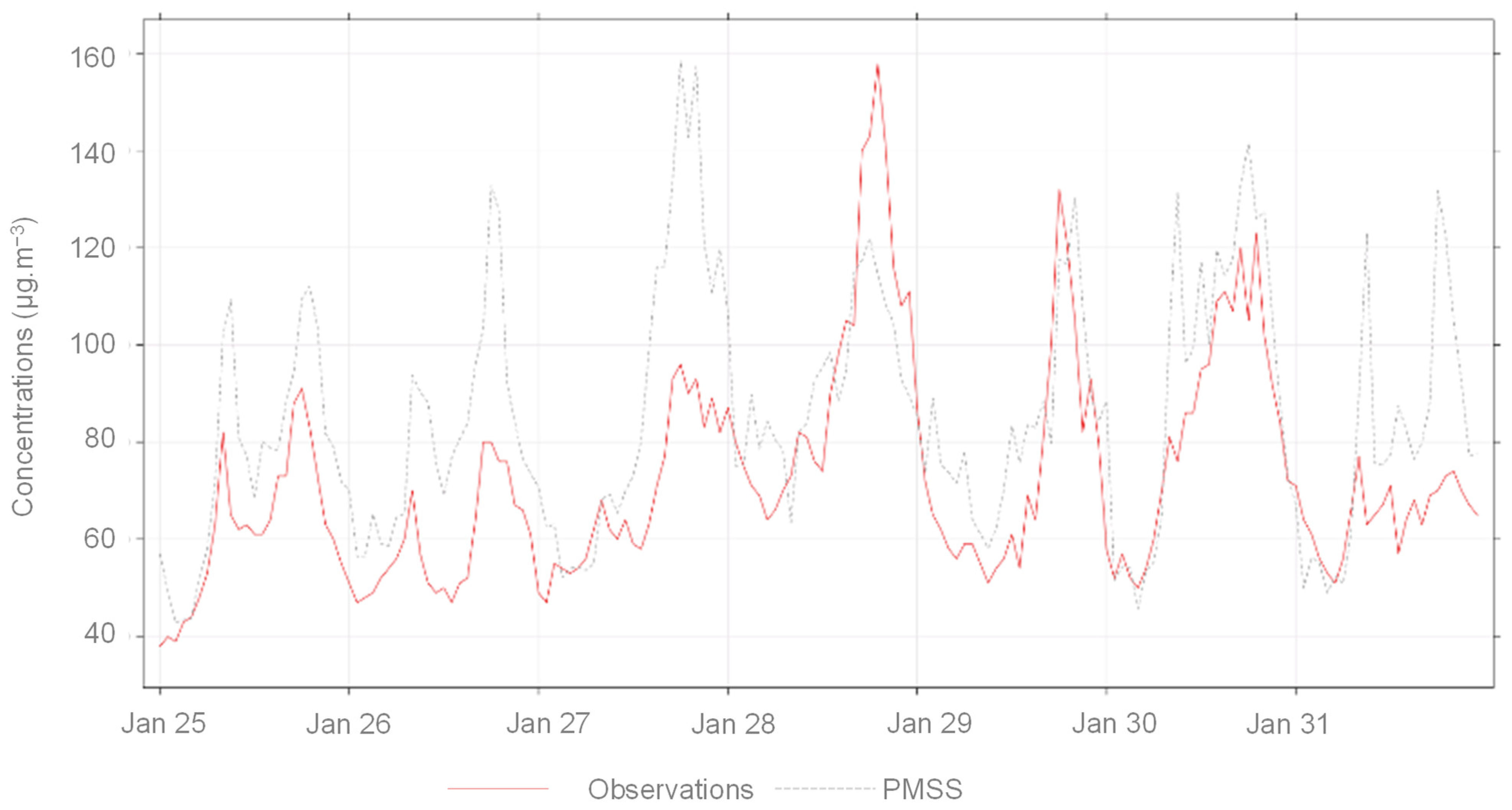
The model-measurement deviations are inferior to 20%, except for the MC_GRE_JPerrot station, where the error exceeds 50%. A strong correlation is observed with an overestimation trend (see Figure 3). All the comparison stations are located close to traffic. Only the Mob_Grenoble_caserne_Bonne is an urban background type. For this station, where scores are the best (see Table 3), regional modelling quality might be preponderant. At the fixed station Grenobles_Boulevard, the hourly evolution of modelled concentrations reproduces well those of the observed concentrations (see Figure 4). If the absolute values of the concentrations are not properly reproduced on the peaks, the temporality is satisfactory.
PMSS NO2 results are compared to SIRANE results obtained by Atmo AURA over the same computation period with strictly the same input data (emissions, meteorology, and background concentrations) (see Figure 5). Only the first vertical level of the PMSS model is compared to the concentrations of the SIRANE model, which correspond more by construction to spatial averages within each street.
At the MC_GRE_JPerrot station, an overestimation with both models is observed. At the MC_GRE_Leclerc station, where PMSS presents an underestimation compared to SIRANE, PMSS input data was therefore reviewed, allowing for the notification of an underestimation of the pollutant mass rates in the neighborhood because of the position at the boundary of the calculation subdomain. The contribution of some near-road sections is missing.
At the Grenoble_Boulevards reference station, it is interesting to observe a good agreement for SIRANE, and an overestimation for PMSS. It is also interesting to analyze the geometric definition of the emission strands in this street, which is, in real life, organized into two traffic lanes separated by two tramway lanes at the center of the street. In the input data, the emissions from both directions are allocated to a single strand, which is itself off-centered and located near the measuring station on one of the sidewalks. In the database, most of the streets are taken into account by a single emission strand, as the SIRANE model considers a balance per street. This might explain the difference observed in the comparison between the two models.
Average concentration maps over the period (see Figure 6) have been calculated by only taking into account the results of the models, without adding the regional background. This enables a better comparison between the specificities of each model. The SIRANE map resolution is 10 m, whereas the PMSS one is 3 m. For the same color scale, concentrations are more contrasted with the PMSS model compared to the SIRANE model (higher concentrations on the road delineation, and zero in buildings). The decrease in concentrations obtained by moving away from a road is more abrupt with the PMSS model, where the SIRANE model further dilutes the concentrations within the streets. This difference not only originates from the resolution difference between the two models, but also, perhaps, from the different modelling principles.

2.4. Rome Case

2.4.1. Context and Model Setup

In the framework of the BEEP project (Big Data in Environmental and Occupational Epidemiology, https://www.progettobeep.it/index.php (accessed on 10 September 2021), 2019), a long-term simulation at building-resolving scale over a large domain that covers most of the Rome conurbation has been run. The simulation has been conducted for the entire year 2015 over a 12 × 12 km urban domain with a high spatial resolution of 4 m grid step, and provides hourly ground concentration fields for different pollutants. The resulting fields account for the concentration values in cells between 0 and 3 m in height, but the domain extends in height up to 300 m, therefore, the calculation grid considers 1.8 × 10⁷ cells.
The simulation has been carried out using a hybrid modelling approach to reproduce air quality of an urban area. The developed hybrid modelling system (HMS) couples PMSS with the Eulerian chemical transport model (CTM) and FARM (flexible air quality regional model) [34,35]. The latter reproduces the transport and the chemical interactions at regional scale of all the sources that are discretized only at the resolution of the CTM, such as the space heating. PMSS simulates, instead, traffic emissions within the city, which cause hotspots and strong concentration gradients typical of urban environments, and deals with the presence of buildings that lead to urban canyon effects. The two models have been run independently, and subsequently combined, allowing the application of each model over a different domain with appropriate grid resolution, and with proper emission inputs. The consistency between the models is ensured by using the same meteorological data, provided by the WRF meteorological model [36], as well as the same topography and land use data for both models. Consequently, FARM considers a 60 × 60 km domain centered over Rome with a horizontal resolution of 1 km, whereas PMSS is applied over the target domain described above.
The advantage of the models’ independent execution is minimizing the computational effort, making it feasible to run long-term microscale simulations over large domains. In fact, a CTM, which requests a lower computational time, manages a greater number of sources, whereas a LPDM, which is more demanding, simulates only traffic emissions. Accordingly, PMSS computational time is representative of that of HMS. In this work, FARM computational time is equal to 11 min per simulated day on an HPC system with 1 node and 36 cores, whereas PMSS takes 3 h per simulated day on an HPC system with 5 nodes and 180 cores. Furthermore, PMSS computational demand is particularly low in respect to traditional implementations, thanks to the exploitation of the kernel method to calculate concentrations inside PMSS code [37]: for this simulation, the deployment of this method has allowed a reduction estimated at about 80% of the computational time compared to what would be obtained using the traditional PMSS code.

2.4.2. Results

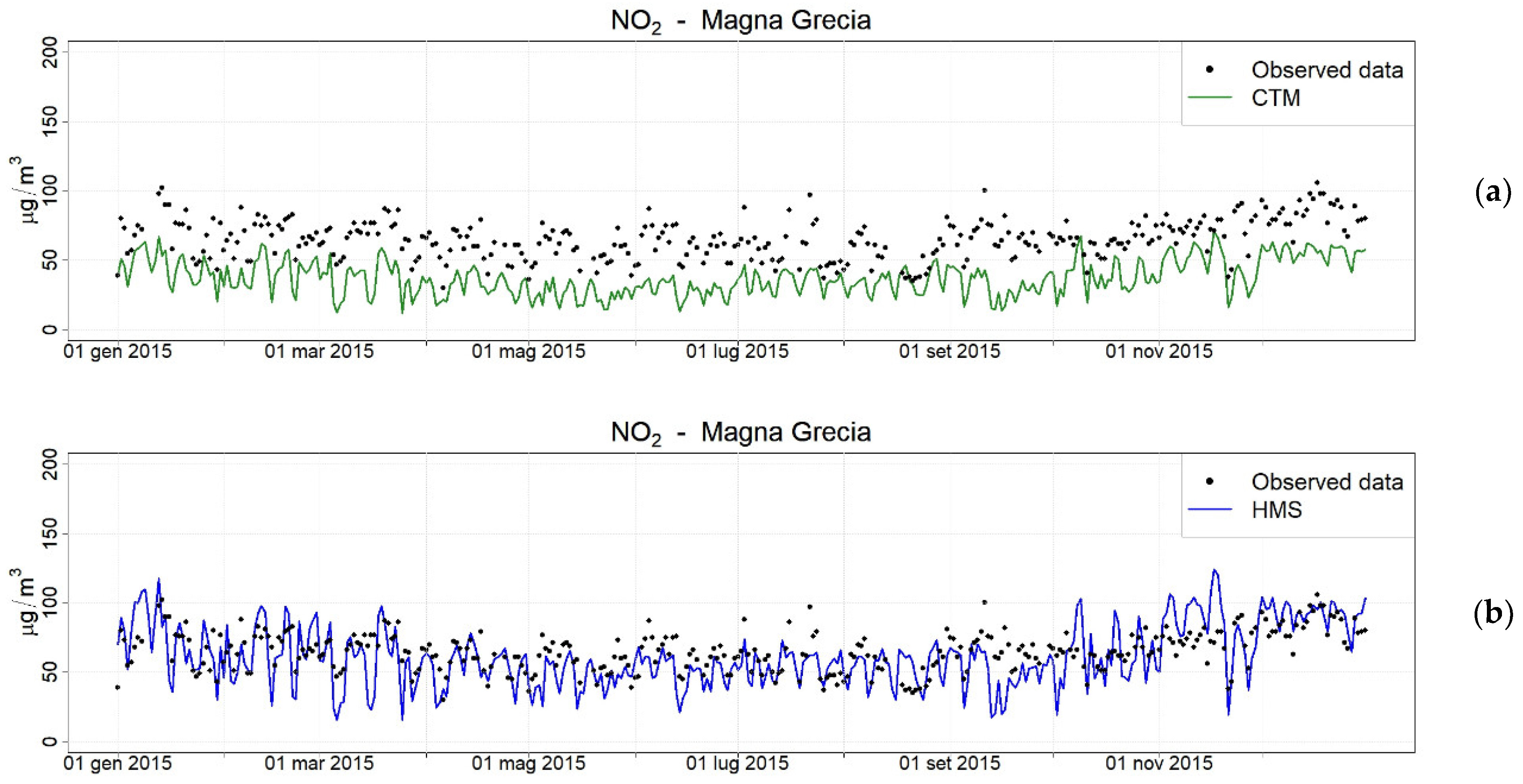
The HMS achieved good performance when reconstructing the typical urban spatial variability, showing very diverse concentration levels in different neighborhoods across the city. The comparison of HMS outcomes with the results of a CTM run at urban scale (typically of 1 km) is particularly promising, mainly due to the fact that the HMS is capable of reproducing the presence of city hotspots, contrarily to a CTM, which is unable to capture these because of its coarser horizontal resolution. Figure 7 shows the comparison between observed and two predicted daily NO2 concentrations during the entire year 2015 at Magna Grecia station, which belongs to the air quality monitoring system of this region, and which is located near a main road. The figure reports the concentrations calculated with FARM in green, run at 1 km of horizontal resolution, and taking into account all the emissions considered by the HMS, and the HMS concentrations are in blue. From this comparison, it is evident that the CTM itself underestimates NO2 concentrations at this urban traffic station, whereas HMS, mainly thanks to PMSS, which better reproduces traffic contribution, has a good agreement with measurements.
Table 4 reports the statistical evaluation of HMS performance on the urban traffic station of Magna Grecia for daily NO2 concentrations, carried out with the estimation of bias, RMSE, and correlation. It confirms the good agreement of HMS results with measurements.

3. REX from Different Forecast Systems

Using a full deterministic approach to forecast physical phenomena implies the constraint of a CPU time smaller than the real time: the whole modelling chain must be faster than real time.
Contrary to the context of the studies presented in the previous section, the computational time cannot be shortened by modelling only a number of days limited by a classification. Hybrid methods including a statistical part can be used [38]. In this paper, the focus is only on entirely deterministic approaches. Two operational systems on cities are presented in this section. The system operated during the Elise project in Turin in 2015–2016 gives an additional example, not detailed here, but described in [39].

3.1. Paris Forecast System

3.1.1. Context and Model Setup

A forecasting system was operated in Paris between September 2018 and January 2019 as part of the FUI FAIRCITY project. It partly takes the configuration setup previously used during the FEDER AIRCITY project [11]: the extent of the calculation domain of the PMSS model is 14,022 m × 11,499 m, including the whole city of Paris. The horizontal spatial resolution is constant, and equal to 3 m. The vertical spatial resolution is of 2 m between the ground, and the first 30 m then decreases until the calculation ceiling, located at 800 m. The mesh counts approximately 6.27 × 10⁸ cells. The calculation chronology allows the calculation of the 24 h of the following day during the night. The system provides hourly concentrations.
Large-scale meteorological data and background concentrations of NO, NO2, O3, and PM10 are taken from the ESMERALDA forecast system of AIRPARIF (http://www.esmeralda-web.fr/accueil/index.php (accessed on 10 September 2021). They are available around 10 PM, local time. Emissions considered by the PMSS model are limited to those from road traffic. The pollutant emissions are estimated by AIRPARIF with the help of a classification by standard day (as opposed to quasi-real-time estimates using real-time-existing measurements of the vehicles fluxes that are not available for the forecasting system). All the input data are available at an hourly time resolution.
The period of several months was leveraged to make the computational workflow more robust. Malfunctions were analyzed and, if possible, led to calculation chain upgrades. Among the malfunctions, those that come from the hardware can be cited (under-sizing of the memory requested to the calculation server: a safety margin has been put into place; crash of a computational node of the calculation server: one occurrence without possible patch; AIRPARIF ftp server does not provide access to the ESMERALDA forecast: two disfunctions), and those that come from the software can be cited (case of a very weak wind leading to PMSS error: three crashes before setting up a patch). The chronology of the malfunctions of the calculation system over the targeted period was: six in September, four in October, one in November, and none in December and January.
The results, in terms of NO2 and PM10 concentrations, were quantitatively analyzed by comparison to observations at the location of AIRPARIF monitoring stations, qualitatively, through the observation of hourly average maps.

3.1.2. Results

Over the period between the 1 September 2018 and the 30 January 2019, the comparison of statistics at monitoring stations, from which we can distinguish those close to the traffic and those in the background, shows a significant over-estimation trend (see Table 5). The over-estimation is lower for the background stations, but present for NO2 and PM10. The models’ calculation cost has greatly limited the number of sensitivity tests that could be carried out afterward. The following paragraphs present some attempts to improve the modelling chain.
Background concentrations added hour by hour to the PMSS results could explain a part of the over-estimation. Modifying them does not require a recalculation, but only post-treatments. Scores at the measuring stations could be recalculated over the entire period with a different method of background estimation: instead of extracting the cell value of the ESMERALDA chain (horizontal resolution of 15 km in the available nesting level early enough for the PMSS forecast chain) located in downtown Paris, we have extracted the cell values upwind of Paris, according to the wind prediction from the ESMERALDA chain. This new calculation, therefore, remains compatible with a forecast mode. It allows for the avoidance of doubly counting emissions related to traffic in Paris, considered both with PMSS and ESMERALDA. Inversely, it does not allow for the inclusion of sources in the PMSS domain but not considered by PMSS, such as urban heating. This method permits significant improved RMSEs and biases, except for several background stations, particularly, with the emergence of negative biases for the NO2 (PA_12, PA_13, and PA_18) and PM10 (PA_18) concentrations, which could be explained by the underestimate of sources other than the road traffic previously mentioned.
The significant size of the computation domain and the large size of the number of modelled days constitute a database with a large variability of both geometric and meteorological configurations. The analysis of concentration maps, more particularly, days with major deviations at stations, has enabled the identification of several issues. The main one is the emergence of a large number of concentration accumulation zones in front of buildings, yet not direct neighbors of an emission strand. The settings analysis of PMSS, and, more specifically, the comparison with other setups that do not present this artifact, highlighted the effect of the α stability coefficient in PSWIFT, used during the mass conservation step. In the Paris calculation chain, this coefficient was calculated during a pre-processing step to PSWIFT from the ESMERALDA temperatures profiles and a tabulation indexed on the vertical temperature gradient. This tabulation, derived from an in-house parametric study carried out with confidential data from a wind farm site with a complex terrain, is adapted for the consideration of the stability effect on obstacle avoidance with hill or mountain length scale, but not with a building length scale: for a Froude number lower than 1, an atmospheric flow bypasses an obstacle [40], but, even for a very stable meteorological case, such as a weak wind with a speed of 1 m·s−1 and a vertical gradient of potential temperature of 0.03°·m−1, the Froude number Fr is equal to 1.59 for an obstacle of height h = 20 m, such as Parisian buildings (Fr = 0.31 for h = 100 m). It is therefore convenient to use α coefficient close to 1 in order to calculate the flow around buildings in urban areas.
Over the 5 months modeling period, 5 days were selected by including cases with good and bad scores, and recalculated with α = 1. Accumulation zones have significantly decreased. Scores from the initial setup (called Config 1) limited to the 5 days are available in Table 5 next to the scores obtained with the α coefficient correction and the choice of the background concentration value in the upwind cell of Paris (named Config 2). Config 1 scores, limited to the 5 days, are generally worse than those for the 5-month period. The choice of 5 days is therefore rather penalizing. Over these 5 days, RMSE, bias, and correlation are improved between Config 1 and Config 2, except at the background stations PA_12, PA_13 and PA_18 for NO2, and at PA_18 for PM10. Low scores recorded at the Auteuil station are significantly improved. This station located on the edge of the ring road is not in the vicinity of a building. Nevertheless, it is close to a slope, the ring road there being located in a 10 m recessed zone. Modification of the α coefficient can therefore have an impact on the calculation of the flow in this area.
Another issue that was observed through the analysis of the hourly average concentration maps is the noisy appearance of the values with horizontal gradients from one cell to the other, even in open areas. Emissions might have been not well discretized because of the number of Lagrangian particles being too low. The calculation time constraint limits this number. Possible improvements include the use of the Kernel method [38] for the computation of concentrations from particles, as well as the optimization of the number of particles emitted by each road section. In the setup used for the Paris forecast system, all the strands emit the same number of particles, even if they emit different amounts of pollutants. On the setup presented in the next section, this distribution, according to mass rate, has been implemented and optimized. It allows the balance between computation time and noise in concentration fields to be improved.
Finally, another issue was observed on the hourly average concentration maps: concentration levels on some major roads appear to be potentially very high (exceeds 1000 µg·m−3 in NO2 some days). These roads are associated with rather fast traffic and rather open areas, which are too wide to experience canyon effects (for example Grande Armée Avenue in Neuilly-sur-Seine or Paris Ring Road). The noise, due to the number of lagrangian particles being too low, could explain some of these high values, but it seems also that the impacted zones depend on the wind direction: particle accumulation along the road axis is maximized when the wind is aligned with the axis. One possibility for improvement could be to consider the turbulence induced by the traffic of these road axes, as already done in the canyon type streets (see Section 1), but with a formulation that would be adapted to less-confined areas.

3.2. Antony Forecast System

3.2.1. Context and Model Setup

A forecasting system for the city of Antony, located in the south suburbs of Paris, was operated between the 15 October 2019 and the 16 April 2020 in the framework of the “Numerical Challenge POC & Go on Air Quality”. The extent of the computational domain of the PMSS model is 4300 m × 4800 m. The horizontal spatial resolution is constant, and is equal to 4 m. The vertical resolution is equal to 1.5 m between the ground, and the first 20 m then decreases gradually up to the calculation ceiling, located at 500 m. The mesh is composed of approximately 3.48 × 10⁷ cells.
The computation chronology allows for calculation of the 24 h of the following day overnight. The chain provides hourly concentrations. Meteorological forcing of PMSS is driven by a forecast made with the WRF model, which, itself, is forced by the NCEP/GFS global forecast. Background concentration forecasts are extracted from the forecast of the COPERNICUS Atmosphere Monitoring Service (CAMS) implemented by ECMWF.

3.2.2. CPU Time Performance and Optimization

No reference station of air quality measurement is included in the domain. The validation of the pollutant concentration forecasts could not be done. Nonetheless, this case remains interesting for the optimization aspect of the computational time. The forecast chain has indeed been operated with a machine which has a limited computation capacity: one node of 12 cores. In order to obtain forecasts results on time (the targeted CPU time is 5 h for 24 modelled hours), the number of particles that discretize the dispersion in PSPRAY has been optimized. The particles emission time step, and the number of particles emitted per source (here, per section of road), were adjusted. By default, this number is identical for all sources, even if they have different pollutant mass rates. Some particles therefore have, with this configuration, a more important weight, which can lead to very noisy concentration fields. PSPRAY enables, though pre-processing or internally, to modulate the numbers of emitted particles according to the mass rate of the pollutant. A pre-processing adjustment was applied to the case of Antony, whose domain includes high traffic highways and low traffic residential lanes.

4. CPU Demand Analysis and Estimation

This section summarizes the computation times for the modelling described previously. Only the dispersion part (calculated by PSPRAY) is detailed because it is predominant in this type of application. For the meteorological part with PSWIFT, the optimization of the computation time could be done by the choice of the number/sizes of tiles (i.e., subdomains). However, this has not been carried out on the different cases. Computation times of PSPRAY can be found in Table 6, in hour and hour.core. They are given for the modelling of a day of physical time. Three of the cases were performed on the EOS server at the CALMIP computing center. Different servers were used for the two other cases. Part of the computing times variability can thus come from the variability of machine performances, but this has not been quantified.
To compare the different cases, it is firstly assumed that the computation time increases linearly with the extent of studied area—the table thus provides CPU times per area unit. The resulting values range from 2.4 to 68 h·core·km−2.
Other parameters that seem to significantly affect the computation time are provided: the number of emission sources, normalized by area, in order to compare sites of different sizes; emission time step and synchronization time step (the synchronization time step in PSPRAY allows recording of the position of particles at a regular frequency, which, apart from these moments, move with their own time steps); whether or not the Kernel method was used for the computation of concentrations. The latter takes more time for the concentration calculation, but can allow the number of particles that need to be transported to be reduced (see the larger emission time-step for the Rome study).
The table only provides a sample of five sites, and the number of parameters influencing the computation time is maybe too large to perform a multi-regression. However, a rough approximation of computation time by unit area (conjecturing the CPU time linearity with the calculation domain area) was done, assuming linearity with: (1) the emission sources number; (2) the inverse of the emission time step; (3) the inverse of synchronization time step; and possibly (4) the inverse of the square of the horizontal resolution. These rough approaches underestimate CPU times for the cases of Grenoble and Rome, but are satisfying for the three other cases. In the Rome study, the Kernel method was used, making this case special compared to others.
The goal of these estimates is to quantify, in principle, the CPU cost for a new site, in order to design the required size for the computing machines.

5. Discussion

The different sites presented in the paper provided both validation scores and valuable feedback to improve the modelling and its CPU cost. The scores’ quality appears to be disparate between the sites, but also for the same site: modelling air quality at local scale means dealing with different configurations, even in the same city (narrow canyon streets, complex crossroads, half-buried highways, skyscraper zones, streets with complex emission distribution due to the presence of tramway lanes).
An overestimation tendency seems to be observed. Even if the possible origins are numerous, an underestimation of the turbulence due to road traffic could be one. This effect could be considered in the 3D turbulence fields, or, more simply, by enlarging the emission volumes.
The long-term results analysis has shown some patterns, and provides feedback that has led to model improvements, especially for making the Rockle approach more robust in more geometrical configurations.
The long-term calculations were also useful to analyze the performances of two methods used to improve the CPU cost:
-
Classification with SOMs method to reduce the number of days to be considered. The study provides the quantification of the classification effect on annual average concentration and, more challengingly, on percentiles;
-
Kernel method to compute concentration fields from particle clouds. The obtained CPU times during the BEEP project are attractive. The method, already implemented in other LPDM, such as FLEXPART [41] and LAPMOD [42], should be tested on other sites.
The CPU time of the different sites have been compared, and a tentative estimation has been made from input parameters and characteristics, such as the area, the number of roads, and particle emission time steps. The limited number of sites does not allow a true multi-regression to be calculated, so only a raw linear law is set. The CPU time database should be fed by all the impact studies performed with PMSS, but these values are not available because they are not stored by default.
The 3D approach presented in the paper allows access to detailed 3D concentration fields that open perspectives about health impact and exposure. Exposure, which is the integration of both concentration and population density, is usually performed based on a 2D raster method. The results provided with PMSS can be used differently: as the buildings are seen explicitly, the exposure can be computed by building. The concentration for each building could be the average and maximum concentration around it, for example. Moreover, the exposure can be computed level by level, quantifying the vertical gradient between the first and last floors. During the FAIRCITY project, a first attempt has been made on an area of Grenoble, with ATMO AURA showing some significant gradients (10% reduction between the ground and 18 m.a.g.l. for the NO2 concentration), but no observation was available to validate the results. Observations in wind tunnel experiments are available [43], but might miss some of the processes present in a real street, such as traffic-induced turbulence, or convective flows due to the thermal and radiative effects of buildings. Having a field campaign with sensors at different heights on the façades of buildings, as is described in [44,45,46], would open a great validation perspective.

Author Contributions

Conceptualization: M.N.; Methodology: M.N.; Software: B.R. and D.B.; Validation: M.N., B.R., G.T. and D.B.; Formal Analysis: M.N., B.R., G.T. and D.B.; Writing—Original Draft Preparation: M.N., B.R., L.R., G.T. and D.B.; Writing—Review and Editing: M.N.; Visualization: B.R. and D.B.; Supervision: M.N.; Project administration: J.M. and G.T.; Funding Acquisition: J.M., G.T. and A.A. All authors have read and agreed to the published version of the manuscript.

Funding

The authors would like to thank the FUI, the Auvergne-Rhône-Alpes and Ile-de-France regions for the funding of the FAIRCITY project, and also the National Institute for Insurance against Accidents at Work for the project “BEEP” (project code B72F17000180005).

Institutional Review Board Statement

Not applicable.

Informed Consent Statement

Not applicable.

Data Availability Statement

Air quality observations on Paris are available on https://data-airparif-asso.opendata.arcgis.com/search?tags=mesure (accessed on 10 September 2021).

Acknowledgments

We truly appreciate the help of the three Air quality regional agencies who provided input data of their own modelling systems and participated in the analyses of the results obtained with the 3D model PMSS. The authors would also like to thank the CALMIP HPC teams for their support.

Conflicts of Interest

The authors declare no conflict of interest.

References

  1. Harrison, R.M. Urban atmospheric chemistry: A very special case for study. NPJ Clim. Atmos. Sci. 2018, 1, 20175. [Google Scholar] [CrossRef] [Green Version]
  2. Arya, S.P. Introduction to Micrometeorology; Academic Press: San Diego, CA, USA, 1987; p. 307. [Google Scholar]
  3. Oke, T.R.; Mills, G.; Christensen, A.; Voogt, J.A. Urban Climates; Cambridge University Press: Cambridge, UK, 2017; p. 519. [Google Scholar]
  4. Moussafir, J.; Oldrini, O.; Tinarelli, G.; Sontowski, J.; Dougherty, C. A new operational approach to deal with dispersion around obstacles: The MSS (Micro-Swift-Spray) software suite. In Proceedings of the 9th International Conference on Harmonisation within Atmospheric Dispersion Modelling for Regulatory Purposes, Garmish-Partenkirchen, Germany, 6–10 June 2004; Volume 2, pp. 114–118. [Google Scholar]
  5. Tinarelli, G.; Brusasca, G.; Oldrini, O.; Anfossi, D.; Trini Castelli, S.; Moussafir, J. Micro-swift-spray (MSS) A new modeling system for the simulation of dispersion at microscale, general description and validation. In Proceedings of the 27th CCMS-NATO Meeting, Banff, AB, Canada, 24–29 October 2004. [Google Scholar]
  6. Rockle, R. Bestimmung der Stromungsverhaltnisse im Bereich Komplexer Bebauungsstrukturen. Ph.D. Thesis, Vom Fachbereich Mechanik, der Technischen Hochschule Darmstadt, Darmstadt, Germany, 1990. [Google Scholar]
  7. Oldrini, O.; Olry, C.; Moussafir, J.; Armand, P.; Duchenne, C. Development of PMSS, the parallel version of Micro SWIFT SPRAY. In Proceedings of the 14th International Conference on Harmonisation within Atmospheric Dispersion Modelling for Regulatory Purposes, Kos, Greece, 2–6 October 2011; pp. 443–447. [Google Scholar]
  8. Oldrini, O.; Armand, P.; Duchenne, C.; Olry, C.; Tinarelli, G. Description and preliminary validation of the PMSS fast response parallel atmospheric flow and dispersion solver in complex built-up areas. J. Environ. Fluid Mech. 2017, 17, 997–1014. [Google Scholar] [CrossRef]
  9. Trini Castelli, S.; Armand, P.; Tinarelli, G.; Duchenne, C.; Nibart, M. Validation of a Lagrangian particle dispersion model with wind tunnel and field experiments in urban environment. Atmos. Environ. 2018, 193, 273–289. [Google Scholar] [CrossRef]
  10. Gomez, F.; Ribstein, B.; Makké, L.; Armand, P.; Moussafir, J.; Nibart, M. Simulation of a dense gas chlorine release with a lagrangian particle dispersion model (LPDM). Atmos. Environ. 2021, 244, 117791. [Google Scholar] [CrossRef]
  11. Moussafir, J.; Olry, C.; Nibart, M.; Albergel, A.; Armand, P.; Duchenne, C.; Mahé, F.; Thobois, L.; Loaëc, S.; Oldrini, O. AIRCITY: A Very High Resolution Atmospheric Dispersion Modeling System for Paris. In American Society of Mechanical Engineers, Fluids Engineering Division; FEDSM: Chicago, IL, USA, 2014; Volume 1D. [Google Scholar] [CrossRef] [Green Version]
  12. Geai, P. Méthode d’interpolation et de reconstitution tridimensionnelle d’un champ de vent: Le code d’analyse objective SWIFT. In EDF/DER Internal Report HE34-87; EDF Group: Chatou, France, 1987. [Google Scholar]
  13. Hanna, S.; White, J.; Trolier, J.; Vernot, R.; Brown, M.; Gowardhan, A.; Kaplan, H.; Alexander, Y.; Moussafir, J.; Wang, Y.; et al. Comparisons of JU2003 observations with four diagnostic urban wind flow and Lagrangian particle dispersion models. Atmos. Environ. 2011, 45, 4073–4081. [Google Scholar] [CrossRef]
  14. Berkowicz, R.; Hertel, O.; Larsen, S.; Sørensen, N. Modelling Traffic Pollution in Streets; Ministry of Environment and Energy, National Environmental Research Institute: Roskilde, Denmark, 1997. [Google Scholar]
  15. Rodean, H.C. Stochastic Lagrangian Models of Turbulent Diffusion; American Meteorological Society: Boston, MA, USA, 1996; Volume 45. [Google Scholar]
  16. Anfossi, D.; Desiato, F.; Tinarelli, G.; Brusasca, G.; Ferrero, E.; Sacchetti, D. TRANSALP 1989 experimental campaign Part II: Simulation of a tracer experiment with Lagrangian particle models. Atmos. Environ. 1998, 32, 1157–1166. [Google Scholar] [CrossRef]
  17. Carvalho, J.; Anfossi, D.; Castelli, S.T.; Degrazia, G.A. Application of a model system for the study of transport and diffusion in complex terrain to the TRACT experiment. Atmos. Environ. 2002, 36, 1147–1161. [Google Scholar] [CrossRef]
  18. Ferrero, E.; Anfossi, D. Comparison of PDFs, closures schemes and turbulence parameterizations in Lagrangian Stochastic Models. Int. J. Environ. Pollut. 1998, 9, 384–410. [Google Scholar]
  19. Ferrero, E.; Anfossi, D.; Tinarelli, G. Simulations of Atmospheric Dispersion in an Urban Stable Boundary Layer. Int. J. Environ. Pollut. 2001, 16, 1–6. [Google Scholar] [CrossRef]
  20. Trini Castelli, S.; Anfossi, D.; Ferrero, E. Evaluation of the environmental impact of two different heating scenarios in urban area. Int. J. Environ. Pollut. 2003, 20, 207–217. [Google Scholar] [CrossRef]
  21. Tinarelli, G.; Anfossi, D.; Brusasca, G.; Ferrero, E.; Giostra, U.; Morselli, M.G.; Moussafir, J.; Tampieri, F.; Trombetti, F. Lagrangian particle simulation of tracer dispersion in the lee of a schematic two-dimensional hill. J. Appl. Meteorol. 1994, 33, 744–756. [Google Scholar] [CrossRef] [Green Version]
  22. Tinarelli, G.; Anfossi, D.; Bider, M.; Ferrero, E.; Trini Castelli, S. A new high performance version of the Lagrangian particle dispersion model SPRAY, some case studies. In Air Pollution Modelling and Its Applications XIII; Gryning, S.E., Batchvarova, E., Eds.; Kluwer Academic/Plenum Press: New York, NY, USA, 2000; pp. 499–507. [Google Scholar]
  23. Thomson, D.J. Criteria for the selection of stochastic models of particle trajectories in turbulent flows. J. Fluid Mech. 1987, 180, 529–556. [Google Scholar] [CrossRef]
  24. Kaplan, H.; Olry, C.; Moussafir, J.; Oldrini, O.; Mahé, F.; Albergel, A. Chemical reactions at street scale using a lagrangian particle dispersion model (LPDM). In Proceedings of the 15th International Conference on Harmonization within Atmospheric Dispersion Modeling for Regulatory Purposes, Madrid, Spain, 6–9 May 2013. [Google Scholar]
  25. Benson, P. CALINE4—A Dispersion Model for Predicting Air Pollutant Concentrations near Roadways. Internal Report No FHWA/CA/TL-84/15. 1989. Available online: https://trid.trb.org/view/215944 (accessed on 15 September 2021).
  26. Malherbe, L.; Wroblewski, A.; Letinois, L.; Rouil, L. Evaluation of numerical models used to simulaite atmospheric pollution near roadways 13. In Proceedings of the International Conference on Harmonisation within Atmospheric Dispersion Modelling for Regulatory Purposes (HARMO 13), Paris, France, 1–4 June 2010; pp. 697–700. [Google Scholar]
  27. Hertel, O.; Berkowicz, R. Operational Street Pollution Model (OSPM). In Evaluation of the Model on Data from St. Olavs Street in Oslo, DMU Luft A-135; National Environmental Research Institute: Roskilde, Denmark, 1989. [Google Scholar]
  28. Soulhac, L.; Salizzoni, P.; Cierco, F.-X.; Perkins, R.J. The model SIRANE for atmospheric urban pollutant dispersion: PART I: Presentation of the model. Atmos. Environ. 2011, 45, 7379–7395. [Google Scholar] [CrossRef]
  29. Armand, P.; Commanay, J.; Nibart, M.; Albergel, A.; Achim, P. 3D simulations of pollutants atmospheric dispersion around the buildings of an industrial site comparison of MERCURE CFD approach with Micro-SWIFT-SPRAY semi-empirical approach. In Proceedings of the 11th International Conference on Harmonisation within Atmospheric Dispersion Modelling for Regulatory Purposes (HARMO11), Cambridge, UK, 2–5 July 2007. [Google Scholar]
  30. Kohonen, T. Self-Organizing Maps, 2nd ed.; Springer: Berlin/Heidelberg, Germany, 1997. [Google Scholar]
  31. Yonggang, L.; Weisberg, R.H. A Review of Self-Organizing Map Applications in Meteorology and Oceanography. In Self Organizing Maps: Applications and Novel Algorithm Design; Mwasiagi, J.I., Ed.; IntechOpen: London, UK, 2011; pp. 253–272. [Google Scholar]
  32. Wendum, D.; Moussafir, J. Méthodes d’interpolation spatiale utilisables pour le calcul d’écoulements atmosphériques à moyenne échelle. In EDF Internal Report EDF/DER HE/32-85.22; EDF Group: Chatou, France, 1985. [Google Scholar]
  33. Menut, L.; Bessagnet, B.; Khvorostyanov, D.; Beekmann, M.; Blond, N.; Colette, A.; Coll, I.; Curci, G.; Foret, G.; Hodzic, A.; et al. CHIMERE (2013): A model for regional atmospheric composition modelling. Geosci. Model Dev. 2013, 6, 981–1028. [Google Scholar] [CrossRef] [Green Version]
  34. Gariazzo, C.; Silibello, C.; Finardi, S.; Radice, P.; Piersanti, A.; Calori, G.; Cecinato, A.; Perrino, C.; Nussio, F.; Cagnoli, M.; et al. A gas/aerosol air pollutants study over the urban area of Rome using a comprehensive chemical transport model. Atmos. Environ. 2007, 41, 7286–7303. [Google Scholar] [CrossRef]
  35. Silibello, C.; Calori, G.; Brusasca, G.; Giudici, A.; Angelino, E.; Fossati, G.; Peroni, E.; Buganza, E. Modelling of PM10 Concentrations Over Milano Urban Area Using Two Aerosol Modules. Environ. Model. Softw. 2008, 23, 333–343. [Google Scholar] [CrossRef]
  36. Skamarock, W.C.; Klemp, J.B.; Dudhia, J.; Gill, D.O.; Barker, D.M.; Duda, M.G.; Huang, X.Y.; Wang, W.; Powers, J.G. A Description of the Advanced Research WRF Version 3; NCAR Technical Note NCAR/TN-475+STR; NCAR: Boulder, CO, USA, 2008. [Google Scholar] [CrossRef]
  37. Barbero, D. Sviluppo e Applicazione del Metodo Kernel in Modelli Lagrangiani a Particelle a Scala Locale e a Microscala. Master’s Thesis, Politecnico di Milano, Milan, Italy, 2019. Available online: http://hdl.handle.net/10589/146531 (accessed on 11 September 2021).
  38. Bessagnet, B.; Couvidat, F.; Lemaire, V. A statistical physics approach to perform fast highly-resolved air quality simulations—A new step towards the meta-modelling of chemistry transport models. Environ. Model. Softw. 2019, 116, 100–109. [Google Scholar] [CrossRef]
  39. Carlino, G.; Pallavidino, L.; Prandi, R.; Avidano, A.; Matteucci, G.; Ricchiuti, F.; Bajardi, P.; Bolognini, L.; Elise, P. Micro-scale modelling of urban Air quality to forecast NO2 critical level in traffic Hot-spots. In Proceedings of the Air Quality 2013, Milan, Italy, 14–18 March 2016. [Google Scholar]
  40. Stull, R.B. An Introduction to Boundary Layer; Springer: Dordrecht, The Netherland, 1988. [Google Scholar]
  41. Stohl, A.; Forster, C.; Frank, A.; Seibert, P.; Wotawa, G. Technical note: The Lagrangian particle dispersion model FLEXPART version 6.2. Atmos. Chem. Phys. 2005, 5, 2461–2474. [Google Scholar] [CrossRef] [Green Version]
  42. Bellasio, R.; Bianconi, R. LAPMOD—Manuale D’uso; Technical report of Enviroware-Air Qual; Consult; Enviroware: Concorezzo, Italy, 2017. [Google Scholar]
  43. Soulhac, L.; Méjean, P.; Perkins, R.J. Modelling the transport and dispersion of pollutants in street canyons. Int. J. Environ. Pollut. 2001, 16, 404–416. [Google Scholar] [CrossRef]
  44. Wu, Y.; Hao, J.; Fu, L.; Wang, Z.; Tang, U. Vertical and horizontal profiles of airborne particulate matter near major roads in Macao, China. Atmos. Environ. 2002, 36, 4907–4918. [Google Scholar] [CrossRef]
  45. Tuckett-Jones, B.T. Reade. In City Quality at Height—Lessons for Developers & Planners; Report from WSP; Parsons Brinkerhoff: London, UK, 2017. [Google Scholar]
  46. Wong, P.P.Y.; Lai, P.-C.; Allen, R.; Cheng, W.; Lee, M.; Tsui, A.; Tang, R.; Thach, T.-Q.; Tian, L.; Brauer, M.; et al. Vertical monitoring of traffic-related air pollution (TRAP) in urban street canyons of Hong Kong. Sci. Total Environ. 2019, 670, 696–703. [Google Scholar] [CrossRef] [PubMed] [Green Version]
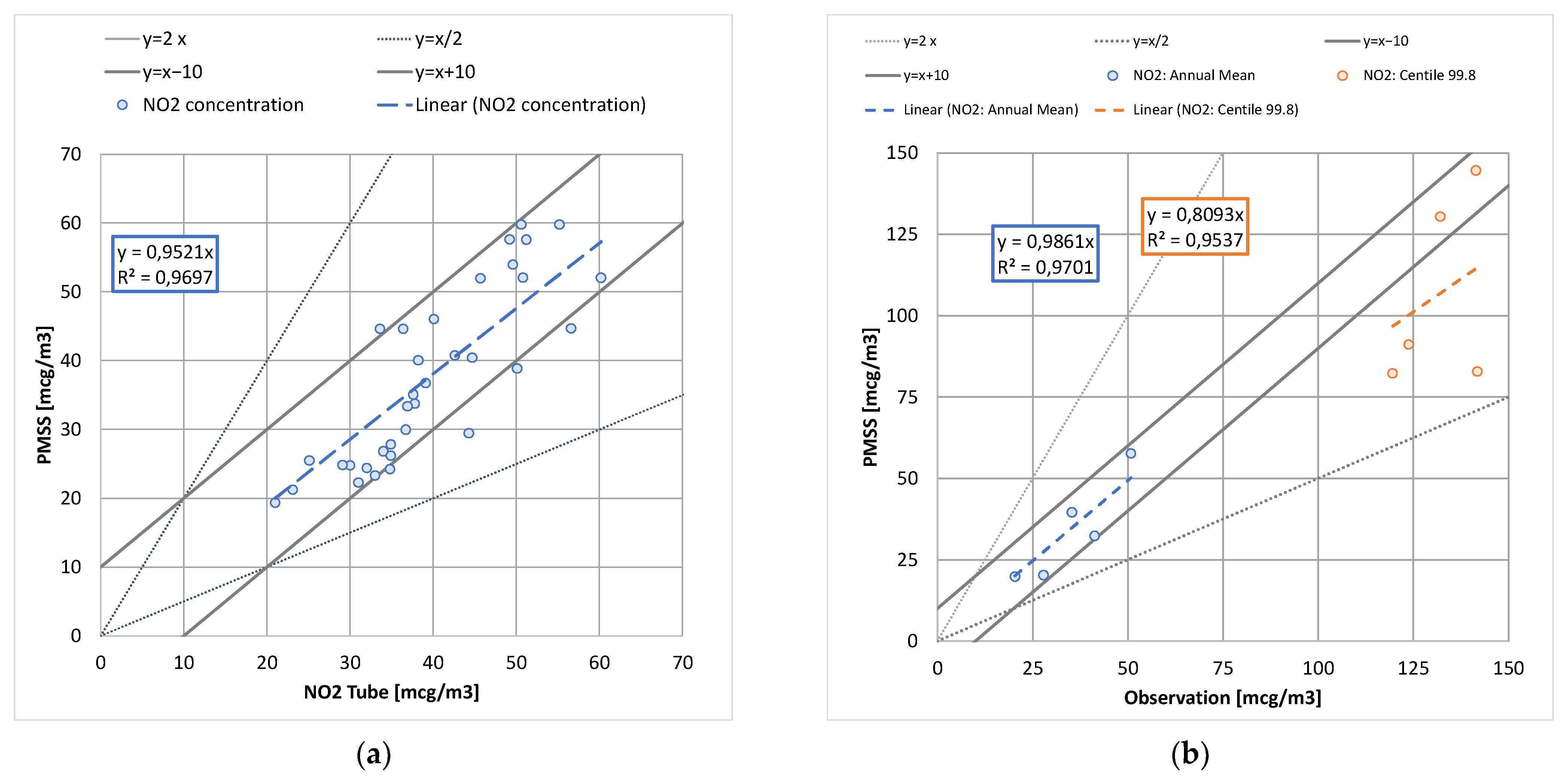
Figure 1. Comparison of observed and computed NO2 concentration for annual average at passive sensors (a), and annual average and 99.8th percentile at monitoring stations (b).
Atmosphere 12 01410 g001
Figure 2. Comparison of annual average (a) and 95th percentile (b) with and without SOMs classification, for different configurations (c1; c2), reconstruction method (m1; m2), and number of target classes (5 × 5; 10 × 10).
Atmosphere 12 01410 g002
Figure 3. Scatter plot observation versus model for all the measurements points (two stations and five micro-sensors)—Hourly average concentration of NO2 during the period from the 15 January 2017 to the 31 January 2017.
Atmosphere 12 01410 g003
Figure 4. Time series of observed and computed concentration of NO2 at Grenoble_boulevards station between the 25 January 2017 and the 31 January 2017.
Atmosphere 12 01410 g004
Figure 5. Average NO2 concentrations during the period from the 15 January 2017 to the 31 January 2017 at measurements points—Observation in blue, PMSS model in orange, and SIRANE model in grey.
Atmosphere 12 01410 g005
Figure 6. Average NO2 concentrations maps during the period from the 15 January 2017 to the 31 January 2017 computed with SIRANE (a) and PMSS (b) models.
Atmosphere 12 01410 g006
Figure 7. Comparison between observed (black dots) and modelled daily NO2 concentrations by the CTM FARM run at 1 km (a) and by HMS (FARM + PMSS) (b) at monitoring station Magna Grecia in Rome.
Atmosphere 12 01410 g007
Table 1. Statistical evaluation of the model performances for hourly NO2 concentrations on five monitoring stations during 359 days of year 2017.
StationMean Observation (µg/m3)Mean Model (µg/m3)Bias (µg/m3)RMSE (µg/m3)r
Station 1 *27.921.4−6.815.460.78
Station 241.333.7−7.624.440.56
Station 3 *20.420.2−0.45.330.95
Station 450.852.92.220.890.68
Station 535.332.8−2.320.100.57
* background stations.
Table 2. List of tested classifications parameters.
Setupc1Wind speed, direction, humidity, and temperature
c2Wind speed, direction, humidity, temperature, and background concentration (PM10, PM25, NO, NO2, O3)
Reconstructionm1A day is equal to the day associated with its representative among the modelled days
m2A day is equal to the weighted sum of the modelled days
Nc5 × 5
10 × 10
Table 3. Statistics of comparison between observed and computed hourly average concentration of NO2 during the period from the 15 January 2017 to the 31 January 2017.
StationMean Observation (µg/m3)Mean Model (µg/m3)Bias (µg/m3)RMSE (µg/m3)r
Grenoble_Boulevards64.976.111.219.90.74
MC_GRE_JJaures53.461.07.613.50.84
MC_GRE_JPain76.572.9−3.624.70.73
MC_GRE_JPerrot40.461.020.623.20.85
MC_GRE_Leclerc52.945.6−7.318.10.77
MC_GRE_VHugo62.063.61.616.20.76
Mob_Grenoble_caserne_Bonne53.853.7−0.18.80.90
Table 4. Statistical evaluation of HMS (FARM + PMSS) performance for daily NO2 values on Magna Grecia station.
StationMean Observation (µg/m3)Mean Model (µg/m3)Bias (µg/m3)RMSE (µg/m3)r
Magna Grecia65.261.6−3.618.780.56
Table 5. Comparative statistics between observed and computed hourly average concentration of NO2 and PM10 in µg·m−3—Config 1 corresponds to the initial parametrization of PMSS and background concentration extracted on Paris cell in the regional modelling; Config 1 Upwind background corresponds to the same parametrization of PMSS, but with background concentration extracted upwind Paris cell in the regional modelling; Config 2 corresponds to the parametrization of PMSS with a correction on the stability coefficient, and with background concentration extracted from the upwind Paris cell in the regional modelling; 5 months and 5 days corresponds, respectively, to the large period modelled initially, and to the sub list of 5 days used afterward.
Period 5 Months5 Days
ObsModel Config 1Model Config 1 Upwind BackgroundModel Config 1Model Config 2
MeanMeanRMSEBiasrMeanRMSEBiasrMeanRMSEBiasrMeanRMSEBiasr
NO2_AUT81.6124.477.243.70.34103.469.231.40.35127.393.653.2−0.0288.531.115.70.62
NO2_BONAP48.567.722.212.10.6544.819.9−0.20.6074.828.121.30.8455.514.25.00.82
NO2_CELES58.781.726.118.60.8055.819.96.60.7771.524.619.30.8058.914.26.50.77
NO2_ELYS47.573.136.525.90.5457.630.113.70.4870.133.024.90.5266.229.421.20.72
NO2_HAUS51.666.328.115.10.6651.523.02.90.6382.341.432.50.5163.825.814.00.58
NO2_OPERA64.999.947.535.50.6681.939.523.40.63104.754.543.30.5694.645.133.50.68
NO2_PA04C *39.346.917.97.80.6133.816.7−4.30.5554.223.115.20.4733.211.6−6.30.78
NO2_PA07 *34.851.129.416.40.3537.625.84.20.2857.931.525.70.6736.318.13.90.61
NO2_PA12 *38.240.817.13.00.5828.219.1−9.20.5346.313.48.70.8126.213.7−11.40.87
NO2_PA13 *35.838.416.23.00.5826.118.7−9.20.5241.213.05.80.7325.113.7−10.50.82
NO2_PA18 *41.534.914.6−5.20.7226.723.2−17.40.6435.39.2−1.80.8019.222.0−17.70.68
PM10_AUT37.251.029.914.30.4444.727.110.10.4353.135.518.40.3138.819.24.40.45
PM10_ELYS31.036.616.15.30.5531.714.70.90.5435.121.98.90.4332.018.35.70.47
PM10_HAUS30.634.415.14.00.5629.713.9−0.20.5337.118.48.50.7230.513.11.70.71
PM10_OPERA29.741.019.011.70.6335.716.17.50.6141.824.314.20.6437.020.29.40.60
PM10_PA04C *21.328.916.37.90.4824.714.53.70.4228.719.210.40.6921.613.22.90.67
PM10_PA18 *21.117.98.4−2.50.7623.511.4−6.70.6715.96.4−1.50.819.212.7−8.30.51
* background stations.
Table 6. Modelling setup parameters, effective CPU demand for dispersion part with PSPRAY model, and estimation through a simple linear fit. The CALMIP calculation center server used is EOS. It is constituted of nodes with Intel IvyBridge @2.80 GHz (20 logical cores per node). The server1 and server2 are internal calculation servers, respectively constituted of two intel Xeon E5-2640 V4 @2.40 GHz (40 logical cores) and two Intel Xeon X5680 @3.33 GHz (12 physical cores without hyperthreading). The two last lines give estimations of CPU based on input parameters and a simple linear fit.
ParisCoastal CityGrenobleAntonyRome
VariableShort NameUnit
Domain X-axis dimensionLxkm103.61.74.312
Domain Y-axis dimensionLykm134.61.84.812
Horizontal resolutiondxm33344
Number of tiles 12091936
Number of line sources per unit areanblinkm−2327.71078.6260.8454.4513.9
Number of emitted particles is function of mass rate nononoyesyes
Kernel method nonononoyes
Emission time stepdtmins210110100
Synchronisation time stepdtsyncs655105
Number of cores 4802403010180
Machine CALMIPCALMIPServer 1Server 2CALMIP
CPU time for 24 h (PSPRAY only) hour6.01.46.95.03.0
Number of hour·core for 24 h hour·core288033320850540
Number of hour·core per day and per km2CPU_costhour·core. km−2·day−122.220.168.02.43.8
CPU_cost estimation = f(nblin/dtmin/dtsync/dx2)CPU_cost_estim1hour·core·km−2·day−122.818.043.52.10.5
CPU_cost estimation = f(nblin/dtmin/dtsync/)CPU_cost_estim2hour·core·km−2·day−122.417.742.83.70.8
Publisher’s Note: MDPI stays neutral with regard to jurisdictional claims in published maps and institutional affiliations.