Abstract
Estimation of satellite-based remotely sensed evapotranspiration (ET) as consumptive use has been an integral part of agricultural water management. However, less attention has been given to future predictions of ET at watershed-scales especially since with a changing climate, there are additional challenges to planning and management of water resources. In this paper, we used nine years of total seasonal ET derived using a satellite-based remote sensing model, Mapping Evapotranspiration at Internalized Calibration (METRIC), to develop a Random Forest machine learning model to predict watershed-scale ET into the future. This statistical model used topographic and climate variables in agricultural areas of Lower Yakima, Washington and had a prediction accuracy of 88% for the region. This model was then used to predict ET into the future with changed climatic conditions under RCP4.5 and RCP8.5 emission scenarios expected by 2050s. The model result shows increases in seasonal ET across some areas of the watershed while decreases in other areas. On average, growing seasonal ET across the watershed was estimated to increase by +5.69% under the low emission scenario (RCP4.5) and +6.95% under the high emission scenario (RCP8.5).
1. Introduction
Water resources are severely stressed particularly in arid and semi-arid regions of the world with diverse competing pressures like agricultural, industrial, municipal, and environmental uses [1,2,3]. Climate change poses an additional risk to water stress and will probably exacerbate water management plans in the future [4,5]. This is because climate change is expected to alter the dynamics of spatiotemporal temperature and precipitation patterns, often resulting in increased evaporative demands [6]. With climate change expected to impose additional limitations on water management activities, it becomes increasingly necessary to predict changes in future agricultural water demands. Moreover, numerous studies have identified water quantity trading as a practical strategy for reducing the detrimental impact of climate change and water shortages [7,8,9,10]. However, uncertainty and complexity in the processes have repercussions in responding to climate change and water shortages [11]. Difficulty in estimating spatiotemporally varied evapotranspiration (ET) at field and watershed scales has led to inefficient water allocation, trading, and other planning operations, which are tremendous concerns in the face of climate variability, change and drought [12,13].
Irrigated agriculture accounts for approximately 80–85% of consumptive water use [14,15] making ET an important measure for agricultural water management. ET is a significant part of the water balance and is therefore essential for predicting water yields, designing water supply, and managing water quantity and quality in watersheds [16,17,18,19]. Therefore, accurate estimation of ET is critical for better agricultural water management both now and in the future. Despite continuing efforts to improve estimation procedures, watershed scale ET is still difficult to determine using measured data and even more difficult to predict due to its spatial and temporal complexity. ET can be modeled using data from weather stations and can be measured directly with high accuracy at specific points using lysimeter or eddy covariance stations [20,21,22]. However, spatially explicit information is more useful to water resource managers. Moreover, being able to determine future ET values as a result of climate modeling efforts is required for strategic planning purposes [23]. Traditional methods for estimating watershed-scale ET addresses these needs by estimating crop coefficients (Kc) over the watershed and multiplying them by a reference ET value at the nearest weather station. Since variability of watershed properties and crop growth stages cannot be accommodated completely into one factor of Kc, alternative approaches for estimating watershed scale ET has been employed—such as the Antecedent Precipitation Index, Advection-Aridity actual ET model [24,25,26] or physically based spatial models like VIC-CropSyst [27] or remote sensing models like METRIC, SEBAL, TSEB, etc. [28,29,30]. Empirical models predicting actual ET and physically-based spatial models, when being used on a larger watershed scale, however, require huge amounts of data, careful consideration of assumptions based on the region of study, and extensive calibration effort [22,27]. Remote sensing approaches have been shown to overcome some of these limitations of physically-based models and perform consistently better with less effort towards calibration or requirement for additional data [31,32]. However, physically-based models have been used extensively in the prediction of ET into the future but use of remote sensing methods to do the same is not yet possible. This study presents a unique approach to use remote sensing with statistical modeling to predict ET into the future that requires much less computational effort than physically-based models.
Due to the complexity of ET estimation, there is increasing interest in the use of machine learning algorithms for robust prediction. Several studies have used statistical and machine learning approaches to predict reference ET and energy balance processes [19,33,34,35]. However, as described by Kumar et al. [36] these models are unable to describe the physical relationship between different components of the process due to the nature of machine learning techniques. Therefore, a model trained with inputs from a specific location cannot be used in a different region without local training Jain et al. [37]. Additionally, these approaches still require extrapolation of ET from point to watershed-scale using Kc. ET values resulting from these models represent the climatic conditions of the locations close to the weather station while the Kc are estimated for specific crop conditions based on the time in the growing season. A few studies have attempted to upscale point measurements of ET to regional scale using climatic predictors and machine learning [38,39] but these studies have used hourly or sub-hourly temporal scale climate variables to estimate regional ET. Since it is impossible to predict climate variables at such fine temporal scale several years into the future, these upscaling methods are not feasible for future prediction of watershed scale ET. Similarly, a few studies have used machine learning techniques to estimate ET between days when satellite imagery is available [40], but these models cannot predict the future due to the lack of imagery. To our knowledge, there are no studies that have used remote sensing models to predict future water consumption in a watershed. A key research question of this paper is to develop a model based on remote sensing information to predict crop consumptive use in agricultural watershed. However, as pointed out by Hindman [41], robust model prediction requires a good set of both response data and predictor variables.
Multiple approaches for determining evapotranspiration using remote sensing technologies have been proposed in the literature [29,42,43,44]. One of these approaches, an energy balance model that uses Landsat imagery called Mapping Evapotranspiration at Internalized Calibration (METRIC) [45], has been used to quantify agricultural consumptive use for decision-making where the results were even upheld in the courts [46,47]. METRIC [45] is specifically designed and parametrized for agricultural areas and has been proven to be reliable as an operational model for producing ET maps at field resolutions across large regions [32]. Here, we use the METRIC ET as the response variable to train a machine learning model to predict the consumptive use of water. Similarly, predictor variables are chosen ranging from topographical, climatic and crop, based on the watershed properties.
The objective of this paper is to develop a predictive model for crop consumptive use in agricultural watersheds and subsequently predict the effect of climate change on crop consumptive use. We developed a random forest model using topographic, climate and crop variables as predictors and METRIC ET as the response. The predictors thus determined are used for estimating the effects of climate change on future consumptive use of water using forecasted climate variables. To provide proof-of-concept for potential watershed-scale forecasting, we focused on agricultural area of Lower Yakima River Basin in Washington State where we trained the Random Forest (RF) model using a growing period dataset of 2008–2014 and tested using the growing period dataset of 2015 and 2016. We make a significant advance on previous studies by developing a framework to predict regional scale ET estimates using climate, topographic and cropping patterns. Using 2008–2014 as the baseline period, we estimated the change in ET in the 2050s with climate projection data for two greenhouse gas emission scenarios (RCP4.5 and RCP8.5). Our study can have multiple uses including better prediction of future water demands and identification of the probable areas for water markets.
2. Materials and Methods
2.1. Study Area
While we believe our approach would be valid for most arid and semi-arid regions, this study focused on the Lower Yakima River basin in the Pacific Northwest U.S. This area is a highly developed watershed for irrigated agriculture and has multiple stakeholders which makes water management a complex issue. There are five upstream reservoirs in the Yakima River basin that account for holding 30% of the mean annual runoff of the system [9]. Moreover, an estimated 97% of water withdrawals from the Yakima River is used in irrigated agriculture [48]. Thus, predicting the impact of climate change on consumptive use of water would be useful to the water managers in the region as storage is highly susceptible to climate change. Besides, the heterogeneity of crops, water rights, irrigation practices, and management decisions of different irrigation districts would make the study applicable in more watersheds.
The 7606 km2 (~3000 square miles) watershed located in southcentral Washington encompasses one of the most productive agricultural areas in the State (Figure 1). This region supports a USD 3 billion irrigated agriculture industry and significant crops include apple, corn, alfalfa, hops, grapes and wheat [9]. The region receives an average rainfall of 212 mm (8.35 inches) and snowfall of 584 mm (23 inches). For this study, we focus only on the agricultural areas of the watershed.
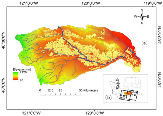
Figure 1.
Study area (Lower Yakima watershed) with agricultural areas highlighted in yellow (a). Location of study area in Washington state with two Landsat image footprints showing the extent of overlap(b).
2.2. Data
2.2.1. Landsat Imagery
Landsat images were used to map ET for our study area due to the high spatial and temporal resolution required. All available Landsat images with cloud cover less than 30% within the Yakima River basin for the growing period of 2008–2016 (mid-April to mid-October) were used. This resulted in Landsat images with path-row 45–28 and 44–28 that covered the agricultural area of the watershed (Figure 1). Google Earth Engine (GEE) [49] was used to access and analyze Landsat data from the public catalog GEE provides using the process implemented in Dhungel and Barber [50].
2.2.2. Weather Data
Hourly and daily weather data required for ET estimation using the METRIC methodology were extracted from two US Bureau of Reclamation (USBR) Agrimet Network weather stations at Harrah (HRHW) and Legrow (LEGW) (Table 1).

Table 1.
Weather station detail used in this study.
2.2.3. Gridded Climate Data
Gridded climate data at 4 km resolution required for the Random forest model were extracted from the PRISM dataset [51].
2.2.4. Climate Projection Data
Gridded climate projections (MACAv2-METADATA) from 20 global climate models downscaled using the Multivariate Adaptive Constructed Analogs approach [52] were extracted for two Representative Concentration Pathway (RCP) scenarios (RCP4.5 and RCP8.5). The GCMs considered in evaluating predictive model performance are: bcccsm1-1, bcccsm1-1, BNU-ESM, CanESM2, CCSM4, CNRM-CM5, CSIRO-Mk3-6-0, GFDL-ESM2G, GFDL-ESM2M, HadGEM2-CC365, HadGEM2-ES365, inmcm4, IPSL-CM5A-LR, IPSL-CM5A-MR, IPSL-CM5B-LR, MIROC5, MIROC-ESM, MIROC-ESM-CHEM, MRI-CGCM3, and NorESM1-M. Instead of choosing a single GCM for prediction, we took the equally weighted multi-model mean of the 20 climate models as the multimodal ensemble average outperforms any individual model [53,54,55].
2.2.5. Elevation and Land Use Data
Digital Elevation Model (DEM) data at 30 m resolution was obtained from the USGS National Elevation Dataset. We also used 30 m resolution agricultural land-use pixels and pasture land-use pixels from the 2006–2011 period obtained from the USGS National Land Cover Database to calibrate the model.
2.2.6. Crop Data
The Cropland Data Layer (CDL), available in the GEE catalog from the US Department of Agriculture (USDA) National Agriculture Statistics Service (NASS), was used to identify the five major crops in the study area based on acreage (corn, alfalfa, hops, grapes, apples).
2.3. METRIC Model
METRIC [46] is an image processing tool for mapping regional ET as a residual of energy balance at the surface (Equation (1)).
where LE is the latent heat flux (W·m−2), Rn is the net radiation (W·m−2), G is the soil heat flux (W·m−2), and H is the sensible heat flux (W·m−2). LE is divided by latent heat of vaporization to get instantaneous ET. The fraction of ET (ETrF, assumed Constant within one day) is calculated by dividing instantaneous ET by the reference ET (ETr, calculated from the nearby weather station, here computed using the American Society of Civil Engineers (ASCE) standardized alfalfa-based reference ET method). To calculate daily ETrF cubic spline interpolation is performed between ETrF of day of satellite overpass, which is multiplied with daily reference ETr for seasonal ET calculation.
Net Radiation (Rn) is estimated from the sum of the difference between the incoming (Rs ↓) and the reflected outgoing shortwave solar radiation (Rs↑), and the difference between the downwelling atmospheric (RL↓) and the surface-emitted and -reflected longwave radiation (RL ↑) (Equation (2)).
The ground heat flux (G) is calculated as the fraction of net radiation using the following equation:
where Ts is surface temperature, is albedo and NDVI is Normalized vegetation index. The sensible heat flux (H) is the rate of heat loss to the air by convection and conduction due to a temperature difference, which can be calculated as:
where is the density of air (kg·m−3), Cp is the air specific heat (=1004 J·kg−1·K−1), while dT is the difference between the air temperature and the aerodynamic temperature near the surface, (dT = Ta − Ts), and rah is the aerodynamic resistance.
METRIC uses two anchor pixels (hot and cold) for internal calibration and to fix boundary conditions for energy balance eradicating the need for in-depth atmospheric correction of surface temperature and reflectance. The calibration is done by choosing the hot and cold pixels to define the vertical temperature gradient range above the surface. Typically, cold conditions correspond to well-irrigated alfalfa fields ET = ETr (reference evapotranspiration over standardized 0.5 m tall alfalfa) whereas hot conditions correspond to dry bare agricultural fields ET = 0. These two pixels are used as boundary conditions to find temperature gradients (dT) at each pixel which is then used to determine the coefficients of a linear relationship (Equation (5)) to be used to calculate dT across the entire image and subsequently the sensible heat flux.
where a and b are empirical constants and are determined using extreme end conditions i.e., with cold pixel (representing maximum LE) and hot pixel (representing zero LE). An iterative solution approach is then applied at these two anchor pixel locations to determine dT followed by the relationship between dT and Ts. For the selection of anchor pixel locations, we followed the process outlined by Dhungel and Barber [50] where a detailed analysis was performed on the effect of anchor pixel selection on the relationship of dT vs. Ts and subsequently on sensible heat flux (H). This approach provides better understanding of the uncertainty and error in METRIC results due to variability in anchor pixel selection process, which is one of the major sources of error in METRIC.
The iterative process and series of steps in the METRIC process requires large data storage and computational engine. We used Google Earth Engine (GEE) [49] and the associated Python API to develop and implement METRIC in an entirely web-based environment that does not require the use of a personal computational engine. GEE is a cloud-based geospatial processing platform that uses per-pixel algebraic functions with a powerful computational infrastructure optimized for parallel processing of large geospatial datasets. Readers are referred to Dhungel and Barber [50] for more details on the process.
2.4. Random Forest Model
We used the Random Forest (RF) [56] algorithm to develop a predictive model for our study as it has been used to predict climate change effects [57,58] and has been shown to perform better than similar other machine learning techniques Fernández-Delgado et al. [59]. RF has been successfully used in similar activities such as predicting the effect of climate change on species distribution [57,58] and land use/cover classification [60,61].
Random forest is a machine learning technique that can be used for both classification and regression. For our purpose, we use it as a regression tool. RF creates a large number of individual decision trees, each based on a bootstrapped sample of the training data [56,62]. As an ensemble machine learning method, RF is relatively insensitive to noise. Further, as long as the individual decision tree models are kept simple, it does not overfit [63] even when the number of records is not large which is the case for our study. Further, splits within each tree are based on different subsamples of the available variables to reduce correlation between trees and to allow the model to explore minor correlations that might otherwise be ignored. As only a subsample of the observations are used to build each tree, the remaining set of observations (out-of-bag; OOB) can be used to test the model. Model predictive error is quantified by comparing OOB predictions with original response variable. The final prediction model is based on the average of an ensemble of decision trees.
2.5. Model Development
Random Forest model development was done using the “randomForest” [62] package available in R, a statistical programming language [64]. Based on Snow Water Equivalent (SWE) and Palmer Drought Severity Index (PDSI) there were two wet years (2011 and 2016) and two dry years (2014 and 2015) in the period of analysis. Thus, the observed nine years dataset (2008–2016) was split into a training set (2008–2014) and a testing set (2015 and 2016) to evaluate the final model performance. Cross-validation was performed on the training data prior to testing final performance by splitting it into training and testing datasets (train: 80% and test: 20%).
For this study, the annual growing season ET computed using METRIC was used as the response variable and watershed and climate properties were used as the predictor variables. A total of 33 predictor variables were selected based on process and basin characteristics that we assumed could affect ET (Table 2). These were derived using temperature, precipitation, crops and elevation data of the watershed. Table 2 provides detailed information about the input and response variable for the Random Forest model, while Table 3 provides the summary statistics of these variables for both training and testing dataset. Correlations between these predictor variables and their correlation with seasonal ET are shown in Figure 2. While summer maximum temperatures, summer maximum vapor pressure deficits, and crop acreage have higher positive correlation, spring minimum vapor pressure deficits and elevation show a slightly higher negative correlation with ET. These variables are expected to perform better in the random forest model. The correlation plot provides the idea about which predictor value could be deterministic in predicting the ET. However, as RF methods model non-linear relationships which may not be apparent from a linear correlation, we used all the predictor parameters for initial model development and implemented a variable selection routine to select the final variable set.
Table 2.
Input and output variables used in Random Forest model.
Table 3.
Summary statistics of input and output variables for both training and testing datasets.
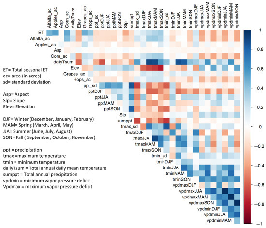
Figure 2.
Correlation matrix of predictor variables.
The 30 m scale ET was upscaled to 4 km scale to have the same scale with climate predictor variables. The upscaling was performed by calculating the total ET from each of the agricultural pixels within the climate variable pixel. As METRIC ET performs well for agricultural areas we masked the METRIC ET with USDA crop layer and used ET values only from agricultural areas.
The next step in model development was selection of model parameters. Variable selection and tuning of model parameters were done using the Variable importance plot and tuneRF method available in the “randomForest” R package [62]. Among all of the variables used in the model, a subset was chosen based on their effect on reduction of Mean Square Error. (MSE) provided as the variable importance plot by the Random Forest package. Since model errors do not decrease significantly after the addition of around 17 variables we selected those 17 variables for our final model. Similarly based on output of tuneRF (Figure 3), we selected tuning parameters the maximum number of terminal nodes (maxnodes) as 10 and number of trees for the forest (ntree) as 100. Since we have a smaller dataset increased number of trees does not affect the computational efficiency and choosing a greater number of trees ensures that every input row gets predicted at least few times.
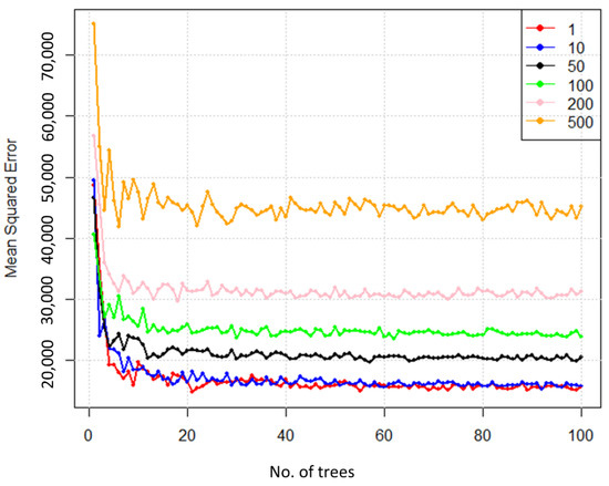
Figure 3.
Tuning of maxnodes and number of trees. Colors in the plot indicate a reduction in MSE error with varying maxnodes.
2.6. Projecting Future Evapotranspiration
Future climate data derived from 20 GCMs for 2051–2060 and for two Representative Concentration Pathway (RCP) scenarios (RCP4.5 and RCP8.5) were used to calculate climate predictor variables identified as important predictors for RF model. To focus only on the effect of climate change we kept the same crop and topographical parameters from the observed period 2008–2014. This was further motivated by the fact that we assume that the crop pattern of major crops (alfalfa, hops, apples, grapes, corn) is unlikely to change substantially over a short period of time. Using the identified current crop and topographical parameters and the projected climate variables, future consumptive uses were computed under present (2008–2014) as well as future time periods and scenarios (2051–2060 for RCP4.5 and RCP8.5). This step was conducted using the “predict” function available in the “randomForest” package in “R” [62]. Here, future predicted evapotranspiration is superimposed on the current evapotranspiration map to assess how climate projections would impact the consumptive use of water.
3. Results
3.1. Historical ET
Figure 4 depicts the METRIC ET values for the growing seasons of 2008–2016 at 4 km scale. METRIC ET was computed at pixel size of Landsat imagery (30 m), but for the purposes of developing the statistical model, it was upscaled from 30 m to 4 km by calculating total ET from each agricultural pixel with the 4 km grid. The spatial variation of evapotranspiration within the watershed and between different years is evident. Evapotranspiration is affected by both climate and supply systems. From Figure 4 we can observe that there are reductions in ET during non-drought periods which could be attributed to the effects of climate change. Similarly, the effects of the supply system on consumptive use are also evident as there are relatively higher ET values on the northern side of the watershed, which is served by the Roza Irrigation District.
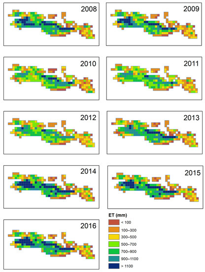
Figure 4.
METRIC ET upscaled from 30 m to 4 km for Lower Yakima River Basin for 2008 to 2016. Each subplot represents the seasonal ET for the corresponding year.
Figure 5 presents the boxplot of the METRIC ET across the study period. From the figure, we can observe that the test dataset of 2015–2016 are in the range of the training dataset of 2008–2014. Since RF model can predict within the range of input variables only. We can expect that the good performance of RF model on test and training dataset. Similarly, variation in the distribution of ET across the years will help in the generalization of the model.
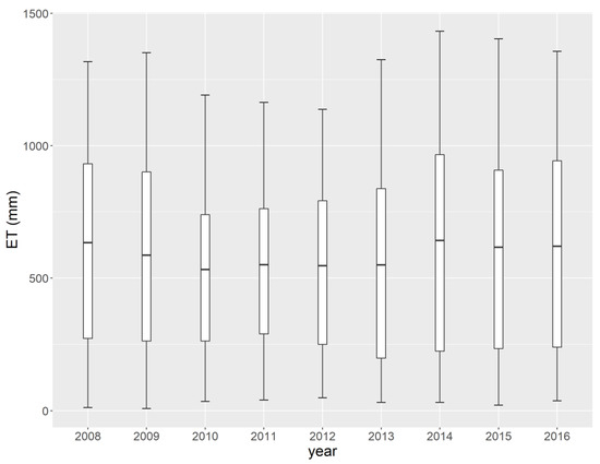
Figure 5.
Distribution plot of 4 km growing seasonal METRIC ET for Lower Yakima River Basin from 2008 to 2016.
3.2. Important Predictors of Watershed ET
Using the variable analysis tools available from the Random Forest package in R, a variable importance plot as shown in Figure 6 was used for selecting the most important variables for the model. The variable importance plot shows the increase in Mean Square Error (MSE) with iterative removal of each predictor in random forest model and sorting them. This results in variables that are considered to have the largest impact on model error to be identified as important predictors. Based on Figure 6, we can identify the important variables for the model which are—(1) apple crop area, (2) corn crop area, (3) hops crop area, (4) slope, (5) grapes crop area, (6) elevation, (7) alfalfa crop area, (8) maximum vapor pressure deficit from September to November, (9) minimum vapor pressure deficit from September to November, (10) minimum temperature from September to November, (11) standard deviation of precipitation, (12) minimum temperature from June to August, (13) aspect, (14) maximum vapor pressure deficit from March to May, (15) standard deviation of maximum temperature, (16) maximum temperature from March to May, and (17) minimum vapor pressure deficit from June to August. These 17 variables were selected as the most important model parameters since additional variables added to the model did not produce significant decreases in the mean square error (MSE). Based on the variable importance plot (Figure 6), we can infer that the most important predictor variables for ET are crop area, basin topography and spring, summer and fall climatic variables. Since the ET values were calculated only from crop pixels, we assume that crop area would have a significant effect on ET. The basin topography parameters slope and aspect determine the amount of radiation received, a major driver of ET. Similarly, temperature is affected by the elevation and thus ET. Since the evaporation from a basin depends upon the precipitation and the temperature, these variables were expected to be important predictors. In addition, the model selected summer and fall climatic variables as important predictors, which is consistent with general consensus that much of the growth and irrigation water application occurs during this time. We also examined the correlation among these variables (Figure 2)and found that all these variables had a correlation coefficient of less than 0.6.
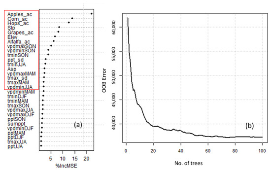
Figure 6.
Variable importance plot for Random Forest with selected variables for final model in red box (a) and reduction of OOB error in the model with an increasing number of trees (b).
3.3. Model Evaluation
The RF model developed in this study could explain about 89% of ET variability using climate and watershed properties. The model’s Out-of-Box (OOB) error levels off as shown in Figure 6 with 80 trees. Figure 7 presents the comparison of RandomForest-predicted-ET with METRIC-ET for two years (2015 and 2016). Overall RF-predicted-ET compared well with METRIC-ET with a Standard Error of Estimate (SEE) of 65 mm (R2: 0.9, slope: 0.74). While 2015 had a SEE of 8.7 mm (R2: 0.92 slope: 0.8), 2016 had a SEE of 83 mm (R2: 0.89, slope: 0.7). Although R2 was ~0.9 for both cases, we can observe from the figure that higher values of ET are underpredicted and lower values of ET are overpredicted by the RF model. This is because prediction by the RF model is based on the average values at the final nodes causing the model to either increase the lowest values or decrease the highest peak values. Therefore, the RF model developed is not good for predicting peak ET values. Nevertheless, it provided a reasonable estimation of the spatial distribution of water use across the watershed. The average difference between METRIC and RF predicted ET for 2015 and 2016~3.5 mm, which is ~0.5% of mean METRIC ET.
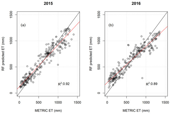
Figure 7.
Performance of RF model to predict METRIC ET for 2015 (a) and 2016 (b). The red line on each subplot is the fitted line and the black line is the line of slope of 1.
3.4. Historical and Projected Climate
Table 4 shows the seasonal average of maximum and minimum temperatures observed for 2008–2014, and the average GCM ensemble maximum and minimum temperatures projected for 2008–2014 and 2051–2060 for our study area. Both the observed and projected temperatures show similar trends although the projected temperatures are slightly higher than the observed. Winter and spring have greater departures whereas summer and fall have the least departures for both maximum and minimum temperatures. In comparison to the 2008–2014 GCM projections, the average increase in maximum temperature projections for RCP4.5 and RCP8.5 for 2051–2060 are 1.62 °C and 2.35 °C, respectively. Similarly, the average increase in minimum temperature for RCP4.5 and RCP8.5 are 1.49 °C and 2.15 °C respectively. As expected, this shows that there is more temperature rise under RCP8.5 (maximum temperature: 0.73 °C, minimum temperature: 0.66 °C) compared to RCP4.5 for 2051–2060.
Table 4.
Average maximum and minimum temperature in °C.
Figure 8 presents the observed and projected precipitation values. While the projected and observed precipitation for the 2008–2014 period are similar during the spring and summer seasons, projected precipitation substantially exceeds the observed precipitation during the fall and winter seasons. A comparison of the projected precipitation for 2008–2014 with 2051–2060 shows that there is little or no change in precipitation during the spring and summer seasons. Whereas, under both scenarios, the precipitation is expected to increase during the winter season. Based on Table 4 and Figure 8 we can expect that our study area will be hotter and drier during the summer and wetter and warmer during the winter.
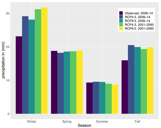
Figure 8.
Barplot of seasonal precipitation.
As depicted in Table 4 and Figure 8, the RCP4.5 and 8.5 climate projections have errors in replicating historic climate conditions. To reduce the impacts of these discrepancies in the climate model projections, we compared the effect of climate change using the low emission scenario RCP4.5 for 2008–2014 data as the baseline and the future forecasted data as the future data. The choice of RCP4.5 is motivated by the fact that it is reasonably close to the original data compared to RCP4.5 for our baseline study.
3.5. Change in Consumptive Use of Water under Future Projected Climate
Figure 9 below shows the predicted change in seasonal consumptive use of water between 2008–2014 and 2051–2060 predicted using the Random Forest statistical model for RCP4.5 and RCP8.5 scenarios. We found that on average the ET increases by 5.69% under RCP4.5 and 6.95% under RCP8.5 scenarios, this is consistent with the increase of temperature for 2051–2060 as shown in Table 4. This will increase the total water demand in the watershed approximately by 130 and 164 million cubic meters of water under the low and high emission scenarios, respectively. The higher value of change in RCP8.5 with respect to RCP4.5 may be because of the effect of a rise in temperature and increasing precipitation in winter. Across the study region, we found that expected change in ET ranges −9.71% to +32.81% when RCP4.5 climate projections are used and between −9.16% to +33.78% when RCP8.5 projections are used. The decrease in ET is noticed around the bottom western region of the study area whereas the increase does not show any discernable pattern. The boxplot in Figure 9 depicts that the distribution of change in ET is expected to be wider under RCP8.5 compared to RCP4.5 scenarios.
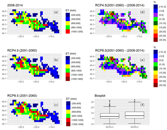
Figure 9.
Change of ET with climate change. (a–c) represent the random forest predicted ET for each climatic scenario. (d,e) represent the percentage change in ET for 2051–2060 with respect to 2008–2014 under RCP4.5 and RCP8.5 scenarios. (f) the boxplot of the percentage change in ET under the two RCP scenarios (black dots present the outlier values).
4. Discussion
Our results show that the future water demand in a watershed increases with the change in climate. We found that in the 2050s there will be an additional water demand of about 130 million cubic meters (110 thousand acre-ft) and about 164 million cubic meters (130 thousand acre-ft) water under the low and high emission scenarios, respectively. With warmer summer and wetter winter projections [65], it can be expected that there will be more water demand in the future, especially during the growing season. This analysis does not factor in any changes in planting dates that may occur due to climate change. Similarly, warmer winter results in less snowfall, quicker snowmelt, and more rainfall. Therefore, it is expected that while there will be an increase in water demand, supplies could dwindle. This necessitates careful and deliberate management of water for future water projects within the watershed. Various water management strategies such as increasing reservoir storage, adopting differing crop patterns, changing management practices, facilitating partial leasing of water rights, groundwater storage and recovery, and improving irrigation efficiency can be employed to manage future water demand [10,66].
Additionally, our results demonstrate that the RF regression model is highly effective for forecasting future evapotranspiration at the watershed scale. A statistical measure of the strength of prediction of future ET using crop acreages and climate data for 2015 and 2016 from this model showed SEE of 65 mm and R2 values greater than 0.9 (Figure 7). The model identified the 17 important variables which influence consumptive use within the selected watershed. Unlike models to estimate potential evapotranspiration, which depends mostly on climate variables, our study showed accurate estimation of actual watershed ET depends on cropping patterns, climate and topography of the area. Removal of any of these variables significantly reduces the accuracy of the model. Moreover, the RF model can also provide useful information about the underlying process and determine the important variables for predicting watershed ET. Another advantage of this model is that, unlike other statistical spatial ET model (support vector machine, extreme learning machine) products [67] which predict potential ET, and requires assumptions of crop coefficients for predictions of actual ET, it provides a direct measure of actual crop ET of the entire watershed. However, there are some limitations to our model.
The Random Forest model developed for our study consistently underpredicted the high values of ET and overpredicted the low values of ET (Figure 7). This is because prediction of regression for the RF model is based on the average of decision trees as well as the inability of the RF model to extrapolate beyond the range of input variables. Thus, the RF model cannot be used to predict peak values in the watershed. Nevertheless, it provides a reasonable estimation of the spatial distribution of water use across the watershed. Although our study is focused on the Yakima region, the model is generalizable to other regions with the understanding that the identified predictor variable will vary. While magnitude and timing of effect of climate change may vary significantly from one basin to another depending upon crop mix, topographical properties of the basin, the results are useful for context such as those in the Yakima River basin where summers are expected to be hotter and winters are expected to be wet and warmer (Table 4 and Figure 8).
Finally, it is important to acknowledge the several necessary simplifications in the decision-making process that were considered beyond the scope of this project. We used the ensemble average mean of the 20 climate models for the projection. This could result in error as only one model could be suitable for the study area and ignores the variation among these, which is a measure of inter-GCM uncertainty. Similarly, we used the METRIC ET as the true ET value. However, there is uncertainty associated with ET estimation using remote sensing model like error due to error in the selection of hot and cold pixel. Nevertheless, we selected hot pixel that had maximum dT and cold pixel that had minimum dT from candidate pixel as the METRIC’s overall performance is better using this selection, we assume that our model is less impacted by error in ET estimation [50]. Besides, in our model, we assume that the ET depends only on the hydrologic characteristics of a particular pixel. However, the supply of water into this basin is not based only on the hydrology of this area but also depends on the reservoir release from the upstream watershed (Upper Yakima), outside our study area. Since statistical models operate only within the bounds of predictor and response space, any change in ET due to change in supply patterns from outside the model space cannot be predicted by this model. In addition, for predicting the future ET we used the same cropping pattern of 2008–2014. While this may not represent the exact change in ET as the cropping pattern may change over time, this will help in predicting the potential change in ET due to the effect of change in the climate.
5. Conclusions
Climate change is likely to alter the dynamics of future water supply and demand around the globe, and thus increase the water stress. While leasing of water rights has been shown to reduce the levels of water stress, the lack of insightful temporal and spatial information on consumptive uses has affected trade flexibility in many watersheds. Information regarding how much water demand will there be in future would allow the better management of water resources with water trading. With the use of Random Forest statistical modeling with a remote sensing model, we have successfully demonstrated the possibility of reliable estimation of future consumptive use of water in facilitating water quantity trading. Superimposing the output of the Random Forest model on observed consumptive use, we predicted the possible change in water demand. We found that on average the future water demand for 2051–2060 will increase by 5.69% and 6.95% percentage under low emission and high emission scenarios respectively.
Researchers and water managers continue finding ways to mitigate the impact of climate change on agricultural water supply and demand. In the future, we hope that this research will lead to alleviating climate change induced water shortage in the watershed. Although this model has been developed for a small area, the same modeling principle can be used to create models in larger spatial domains. This could provide better predictions of change in future actual ET at regional scales. More research and innovations are needed to cope with the climate change induced water shortage.
Author Contributions
Conceptualization: R.K., S.D. and M.E.B. Methodology: R.K., S.D., S.C.B. and M.E.B. Software: R.K. and S.D. Validation: R.K., S.D. and S.C.B. Formal Analysis: R.K., S.D. and M.E.B. Investigation: R.K. and S.D. Resources: M.E.B. Data Curation: R.K. Writing—original draft preparation: R.K. Writing—review and editing: R.K., S.D., S.C.B. and M.E.B. Visualization: R.K. and S.D. Supervision: M.E.B. Project Administration: M.E.B. Funding Acquisition: M.E.B. All authors have read and agreed to the published version of the manuscript.
Funding
This research was supported by the Washington State Department of Ecology, Office of Columbia River and USDA National Institute of Food and Agriculture, project #1016467.
Institutional Review Board Statement
Not applicable.
Informed Consent Statement
Not applicable.
Data Availability Statement
The datas used in this study are publicly available Landsat image (https://earthexplorer.usgs.gov/ accessed on 23 November 2021), PRISM data (https://prism.oregonstate.edu/ accessed on 23 November 2021) and downscaled climate projection data (https://climate.northwestknowledge.net/MACA/data_portal.php accessed on 23 November 2021).
Conflicts of Interest
The authors declare no conflict of interest.
Abbreviations
| CDL | Cropland Data Layer |
| Specific heat of air | |
| DEM | Digital Elevation Model |
| dT | Temperature gradient |
| ET | Evapotranspiration |
| ETr | Reference evapotranspiration |
| G | Sensible heat flux conducted into the ground |
| GCM | General Circulation Model |
| GEE | Google Earth Engine |
| H | Sensible heat flux convected to the air |
| Kc | Crop coefficient |
| LE | Latent Energy |
| maxnodes | Maximum number of terminal nodes |
| METRIC | Mapping Evapotranspiration at Internalized Calibration |
| MSE | Mean Square Error |
| mtry | Number of variables used in splitting |
| NASS | National Agriculture Statistics Service |
| ntree | Number of trees for the forest |
| OOB | Out-of-bag |
| PDSI | Palmer Drought Severity Index |
| RCP | Representative Concentration Pathway |
| R2 | R-square |
| RF | Random Forest |
| Rn | Net Radiation |
| SEBAL | Surface Energy Balance Algorithm for Land |
| SEE | Standard Error of Estimate |
| SWE | Snow Water Equivalent |
| Ts | Surface temperature |
| TSEB | Two-Source Energy Balance |
| USBR | US Bureau of Reclamation |
| USDA | US Department of Agriculture |
| Albedo | |
| Density of air |
References
- Vörösmarty, C.J.; Green, P.; Salisbury, J.; Lammers, R.B. Global Water Resources: Vulnerability from Climate Change and Population Growth. Science 2000, 289, 284–288. [Google Scholar] [CrossRef]
- Scanlon, B.R.; Faunt, C.C.; Longuevergne, L.; Reedy, R.C.; Alley, W.M.; McGuire, V.L.; McMahon, P.B. Groundwater depletion and sustainability of irrigation in the US High Plains and Central Valley. Proc. Natl. Acad. Sci. USA 2012, 109, 9320–9325. [Google Scholar] [CrossRef]
- Flörke, M.; Schneider, C.; McDonald, R.I. Water competition between cities and agriculture driven by climate change and urban growth. Nat. Sustain. 2018, 1, 51–58. [Google Scholar] [CrossRef]
- Crossman, J.; Futter, M.; Oni, S.; Whitehead, P.; Jin, L.; Butterfield, D.; Baulch, H.; Dillon, P. Impacts of climate change on hydrology and water quality: Future proofing management strategies in the Lake Simcoe watershed, Canada. J. Great Lakes Res. 2012, 39, 19–32. [Google Scholar] [CrossRef]
- Rajagopalan, K.; Chinnayakanahalli, K.J.; Stockle, C.O.; Nelson, R.L.; Kruger, C.E.; Brady, M.P.; Malek, K.; Dinesh, S.T.; Barber, M.E.; Hamlet, A.F.; et al. Impacts of Near-Term Climate Change on Irrigation Demands and Crop Yields in the Columbia River Basin. Water Resour. Res. 2018, 54, 2152–2182. [Google Scholar] [CrossRef]
- Collins, M.; Knutti, R.; Arblaster, J.; Dufresne, J.-L.; Fichefet, T.; Friedlingstein, P.; Gao, X.; Gutowski, W.J.; Johns, T.; Krinner, G.; et al. Long-term Climate Change: Projections, Commitments and Irreversibility. In Climate Change 2013: The Physical Science Basis. Contribution of Working Group I to the Fifth Assessment Report of the Intergovernmental Panel on Climate Change; Stocker, T.F., Qin, D., Plattner, G.-K., Tignor, M., Allen, S.K., Boschung, J., Nauels, A., Xia, Y., Bex, V., Midgley, P.M., Eds.; Cambridge University Press: Cambridge, UK; New York, NY, USA, 2013; pp. 1029–1136. [Google Scholar] [CrossRef]
- Pease, M.; Snyder, T. Model Water Transfer Mechanisms as a Drought Preparation System. J. Contemp. Water Res. Educ. 2017, 161, 66–80. [Google Scholar] [CrossRef][Green Version]
- Rey, D.; Holman, I.P.; Knox, J.W. Developing drought resilience in irrigated agriculture in the face of increasing water scarcity. Reg. Environ. Chang. 2017, 17, 1527–1540. [Google Scholar] [CrossRef]
- Yoder, J.; Adam, J.; Brady, M.; Cook, J.; Katz, S.; Johnston, S.; Malek, K.; McMillan, J.; Yang, Q. Benefit-Cost Analysis of Integrated Water Resource Management: Accounting for Interdependence in the Yakima Basin Integrated Plan. JAWRA J. Am. Water Resour. Assoc. 2017, 53, 456–477. [Google Scholar] [CrossRef]
- Khanal, R.; Brady, M.P.; Stöckle, C.O.; Rajagopalan, K.; Yoder, J.; Barber, M.E. The Economic and Environmental Benefits of Partial Leasing of Agricultural Water Rights. Water Resour. Res. 2021, 57. [Google Scholar] [CrossRef]
- Grafton, Q.; Libecap, G.; McGlennon, S.; Landry, C.; O’Brien, B. An Integrated Assessment of Water Markets: A Cross-Country Comparison. Rev. Environ. Econ. Policy 2011, 5, 219–239. [Google Scholar] [CrossRef]
- Knox, J.; Kay, M.; Weatherhead, E. Water regulation, crop production, and agricultural water management—Understanding farmer perspectives on irrigation efficiency. Agric. Water Manag. 2012, 108, 3–8. [Google Scholar] [CrossRef]
- Luo, B.; Maqsood, I.; Yin, Y.Y.; Huang, G.H.; Cohen, S.J. Adaption to Climate Change through Water Trading under Uncertainty An Inexact Two-Stage Nonlinear Programming Approach. J. Environ. Inform. 2015, 2, 58–68. [Google Scholar] [CrossRef]
- Schaible, G.; Aillery, M. Water Conservation in Irrigated Agriculture: Trends and Challenges in the Face of Emerging Demands. SSRN Electron. J. 2012. [Google Scholar] [CrossRef]
- D’Odorico, P.; Chiarelli, D.D.; Rosa, L.; Bini, A.; Zilberman, D.; Rulli, M.C. The global value of water in agriculture. Proc. Natl. Acad. Sci. USA 2020, 117, 21985–21993. [Google Scholar] [CrossRef]
- Syed, T.H.; Webster, P.J.; Famiglietti, J.S. Assessing variability of evapotranspiration over the Ganga river basin using water balance computations. Water Resour. Res. 2014, 50, 2551–2565. [Google Scholar] [CrossRef]
- Singh, R.K.; Senay, G.B.; Velpuri, N.M.; Bohms, S.; Scott, R.L.; Verdin, J.P. Actual Evapotranspiration (Water Use) Assessment of the Colorado River Basin at the Landsat Resolution Using the Operational Simplified Surface Energy Balance Model. Remote Sens. 2013, 6, 233–256. [Google Scholar] [CrossRef]
- Xue, B.-L.; Wang, L.; Li, X.; Yang, K.; Chen, D.; Sun, L. Evaluation of evapotranspiration estimates for two river basins on the Tibetan Plateau by a water balance method. J. Hydrol. 2013, 492, 290–297. [Google Scholar] [CrossRef]
- Torres, A.F.; Walker, W.R.; McKee, M. Forecasting daily potential evapotranspiration using machine learning and limited climatic data. Agric. Water Manag. 2011, 98, 553–562. [Google Scholar] [CrossRef]
- Hirschi, M.; Michel, D.; Lehner, I.; Seneviratne, S.I. A site-level comparison of lysimeter and eddy covariance flux measurements of evapotranspiration. Hydrol. Earth Syst. Sci. 2017, 21, 1809–1825. [Google Scholar] [CrossRef]
- Ding, R.; Kang, S.; Li, F.; Zhang, Y.; Tong, L.; Sun, Q. Evaluating eddy covariance method by large-scale weighing lysimeter in a maize field of northwest China. Agric. Water Manag. 2010, 98, 87–95. [Google Scholar] [CrossRef]
- Mobilia, M.; Longobardi, A. Prediction of Potential and Actual Evapotranspiration Fluxes Using Six Meteorological Data-Based Approaches for a Range of Climate and Land Cover Types. ISPRS Int. J. Geo-Inf. 2021, 10, 192. [Google Scholar] [CrossRef]
- Tian, D.; Martinez, C.J. Forecasting Reference Evapotranspiration Using Retrospective Forecast Analogs in the Southeastern United States. J. Hydrometeorol. 2012, 13, 1874–1892. [Google Scholar] [CrossRef]
- Mawdsley, J.A.; Ali, M.F. Estimating Nonpotential Evapotranspiration by Means of the Equilibrium Evaporation Concept. Water Resour. Res. 1985, 21, 383–391. [Google Scholar] [CrossRef]
- Mobilia, M.; Schmidt, M.; Longobardi, A. Modelling Actual Evapotranspiration Seasonal Variability by Meteorological Data-Based Models. Hydrology 2020, 7, 50. [Google Scholar] [CrossRef]
- Brutsaert, W.; Stricker, H. An advection-aridity approach to estimate actual regional evapotranspiration. Water Resour. Res. 1979, 15, 443–450. [Google Scholar] [CrossRef]
- Malek, K.; Stöckle, C.; Chinnayakanahalli, K.; Nelson, R.; Liu, M.; Rajagopalan, K.; Barik, M.; Adam, J.C. VIC–CropSyst-v2: A regional-scale modeling platform to simulate the nexus of climate, hydrology, cropping systems, and human decisions. Geosci. Model. Dev. 2017, 10, 3059–3084. [Google Scholar] [CrossRef]
- Anderson, M.C.; Kustas, W.P.; Norman, J.M.; Hain, C.R.; Mecikalski, J.R.; Schultz, L.; González-Dugo, M.P.; Cammalleri, C.; D’Urso, G.; Pimstein, A.; et al. Mapping daily evapotranspiration at field to continental scales using geostationary and polar orbiting satellite imagery. Hydrol. Earth Syst. Sci. 2011, 15, 223–239. [Google Scholar] [CrossRef]
- Bastiaanssen, W.; Menenti, M.; Feddes, R.; Holtslag, B. A remote sensing surface energy balance algorithm for land (SEBAL). 1. Formulation. J. Hydrol. 1998, 212–213, 198–212. [Google Scholar] [CrossRef]
- Velpuri, N.M.; Senay, G.B.; Singh, R.K.; Bohms, S.; Verdin, J.P. A comprehensive evaluation of two MODIS evapotranspiration products over the conterminous United States: Using point and gridded FLUXNET and water balance ET. Remote Sens. Environ. 2013, 139, 35–49. [Google Scholar] [CrossRef]
- Dile, Y.T.; Ayana, E.K.; Worqlul, A.W.; Xie, H.; Srinivasan, R.; Lefore, N.; You, L.; Clarke, N. Evaluating satellite-based evapotranspiration estimates for hydrological applications in data-scarce regions: A case in Ethiopia. Sci. Total. Environ. 2020, 743, 140702. [Google Scholar] [CrossRef] [PubMed]
- Dhungel, S. Predicting Watershed-scale Agricultural Water Consumption Using Statistical and Cropping System Models with Satellite-Based Remote Sensing. University of Utah. 2019. Available online: https://www.proquest.com/openview/6127c38237edeb338b37ef083e159a52/1?pq-origsite=gscholar&cbl=18750&diss=y (accessed on 23 November 2021).
- Famiglietti, J.S.; Wood, E.F. Multiscale modeling of spatially variable water and energy balance processes. Water Resour. Res. 1994, 30, 3061–3078. [Google Scholar] [CrossRef]
- Solomatine, D.P.; Shrestha, D.L. A novel method to estimate model uncertainty using machine learning techniques. Water Resour. Res. 2009, 45. [Google Scholar] [CrossRef]
- Abdullah, S.S.; Malek, M.; Abdullah, N.S.; Kisi, O.; Yap, K.S. Extreme Learning Machines: A new approach for prediction of reference evapotranspiration. J. Hydrol. 2015, 527, 184–195. [Google Scholar] [CrossRef]
- Kumar, M.; Raghuwanshi, N.S.; Singh, R. Artificial neural networks approach in evapotranspiration modeling: A review. Irrig. Sci. 2010, 29, 11–25. [Google Scholar] [CrossRef]
- Jain, S.K.; Nayak, P.C.; Sudheer, K.P. Models for estimating evapotranspiration using artificial neural networks, and their physical interpretation. Hydrol. Process. 2008, 22, 2225–2234. [Google Scholar] [CrossRef]
- Xu, T.; Guo, Z.; Liu, S.; He, X.; Meng, Y.; Xu, Z.; Xia, Y.; Xiao, J.; Zhang, Y.; Ma, Y.; et al. Evaluating Different Machine Learning Methods for Upscaling Evapotranspiration from Flux Towers to the Regional Scale. J. Geophys. Res. Atmos. 2018, 123, 8674–8690. [Google Scholar] [CrossRef]
- Bodesheim, P.; Jung, M.; Gans, F.; Mahecha, M.D.; Reichstein, M. Upscaled diurnal cycles of land–atmosphere fluxes: A new global half-hourly data product. Earth Syst. Sci. Data 2018, 10, 1327–1365. [Google Scholar] [CrossRef]
- Bachour, R.; Walker, W.R.; Ticlavilca, A.M.; McKee, M.; Maslova, I. Estimation of Spatially Distributed Evapotranspiration Using Remote Sensing and a Relevance Vector Machine. J. Irrig. Drain. Eng. 2014, 140, 04014029. [Google Scholar] [CrossRef]
- Hindman, M. Building Better Models: Prediction, Replication, and Machine Learning in the Social Sciences. Ann. Am. Acad. Political Soc. Sci. 2015, 659, 48–62. [Google Scholar] [CrossRef]
- Courault, D.; Seguin, B.; Olioso, A. Review on estimation of evapotranspiration from remote sensing data: From empirical to numerical modeling approaches. Irrig. Drain. Syst. 2005, 19, 223–249. [Google Scholar] [CrossRef]
- Senay, G.B.; Bohms, S.; Singh, R.K.; Gowda, P.H.; Velpuri, N.M.; Alemu, H.; Verdin, J.P. Operational Evapotranspiration Mapping Using Remote Sensing and Weather Datasets: A New Parameterization for the SSEB Approach. JAWRA J. Am. Water Resour. Assoc. 2013, 49, 577–591. [Google Scholar] [CrossRef]
- Thorp, K.R.; Thompson, A.L.; Harders, S.J.; French, A.N.; Ward, R.W. High-Throughput Phenotyping of Crop Water Use Efficiency via Multispectral Drone Imagery and a Daily Soil Water Balance Model. Remote Sens. 2018, 10, 1682. [Google Scholar] [CrossRef]
- Allen, R.G.; Tasumi, M.; Trezza, R. Satellite-Based Energy Balance for Mapping Evapotranspiration with Internalized Calibration (METRIC)—Model. J. Irrig. Drain. Eng. 2007, 133, 380–394. [Google Scholar] [CrossRef]
- Allen, R.G.; Tasumi, M.; Morse, A.; Trezza, R. A Landsat-based energy balance and evapotranspiration model in Western US water rights regulation and planning. Irrig. Drain. Syst. 2005, 19, 251–268. [Google Scholar] [CrossRef]
- Liaqat, U.W.; Choi, M. Surface energy fluxes in the Northeast Asia ecosystem: SEBS and METRIC models using Landsat satellite images. Agric. For. Meteorol. 2015, 214-215, 60–79. [Google Scholar] [CrossRef]
- Hillman, B.; Douglas, E.M.; Terkla, D. An analysis of the allocation of Yakima River water in terms of sustainability and economic efficiency. J. Environ. Manag. 2012, 103, 102–112. [Google Scholar] [CrossRef] [PubMed]
- Gorelick, N.; Hancher, M.; Dixon, M.; Ilyushchenko, S.; Thau, D.; Moore, R. Google Earth Engine: Planetary-scale geospatial analysis for everyone. Remote Sens. Environ. 2017, 202, 18–27. [Google Scholar] [CrossRef]
- Dhungel, S.; Barber, M.E. Estimating Calibration Variability in Evapotranspiration Derived from a Satellite-Based Energy Balance Model. Remote Sens. 2018, 10, 1695. [Google Scholar] [CrossRef]
- PRISM Climate Group, Oregon State University. Available online: http://prism.oregonstate.edu (accessed on 23 November 2021).
- Abatzoglou, J.T.; Brown, T.J. A comparison of statistical downscaling methods suited for wildfire applications. Int. J. Clim. 2011, 32, 772–780. [Google Scholar] [CrossRef]
- Herger, N.; Abramowitz, G.; Knutti, R.; Angélil, O.; Lehmann, K.; Sanderson, B.M. Selecting a climate model subset to optimise key ensemble properties. Earth Syst. Dyn. 2018, 9, 135–151. [Google Scholar] [CrossRef]
- Meehl, G.A.; Hu, G.A.M.A.; Santer, B.D.; Xie, S.-P. Contribution of the Interdecadal Pacific Oscillation to twentieth-century global surface temperature trends. Nat. Clim. Chang. 2016, 6, 1005–1008. [Google Scholar] [CrossRef]
- Knutti, R. The end of model democracy? Clim. Chang. 2010, 102, 395–404. [Google Scholar] [CrossRef]
- Breiman, L. Random forests. Mach. Learn. 2001, 45, 5–32. [Google Scholar] [CrossRef]
- Attorre, F.; Alfò, M.; de Sanctis, M.; Francesconi, F.; Valenti, R.; Vitale, M.; Bruno, F. Evaluating the effects of climate change on tree species abundance and distribution in the Italian peninsula. Appl. Veg. Sci. 2011, 14, 242–255. [Google Scholar] [CrossRef]
- Evans, J.S.; Murphy, M.A.; Holden, Z.A.; Cushman, S.A. Modeling Species Distribution and Change Using Random Forest. In Predictive Species and Habitat Modeling in Landscape Ecology: Concepts and Applications; Drew, C.A., Wiersma, Y.F., Huettmann, F., Eds.; Springer: New York, NY, USA, 2011; pp. 139–159. [Google Scholar] [CrossRef]
- Fernández-Delgado, M.; Cernadas, E.; Barro, S.; Amorim, D. Do we need hundreds of classifiers to solve real world classification problems? J. Mach. Learn. Res. 2014, 15, 3133–3181. [Google Scholar]
- Nitze, I.; Barrett, B.; Cawkwell, F. Temporal optimisation of image acquisition for land cover classification with Random Forest and MODIS time-series. Int. J. Appl. Earth Obs. Geoinf. 2015, 34, 136–146. [Google Scholar] [CrossRef]
- Rodriguez-Galiano, V.F.; Ghimire, B.; Rogan, J.; Chica-Olmo, M.; Rigol-Sanchez, J.P. An assessment of the effectiveness of a random forest classifier for land-cover classification. ISPRS J. Photogramm. Remote Sens. 2012, 67, 93–104. [Google Scholar] [CrossRef]
- Liaw, A.; Wiener, M. Classification and Regression by RandomForest. Forest 2002, 23, 18–22. [Google Scholar]
- Watts, J.; Lawrence, R. Merging random forest classification with an object-oriented approach for analysis of agricultural lands. Int. Arch. Photogramm. Remote Sens. Spat. Inf. Sci. 2008, 37, 579–582. [Google Scholar]
- R Core Team. R: A Language and Environment for Statistical Computing 2020; Foundation for Statistical Computing: Vienna, Austria, 2019. [Google Scholar]
- Abatzoglou, J.; Rupp, D.E.; Mote, P.W. Seasonal Climate Variability and Change in the Pacific Northwest of the United States. J. Clim. 2014, 27, 2125–2142. [Google Scholar] [CrossRef]
- Lane, B.A.; Rosenberg, D.E. Promoting In-Stream Flows in the Changing Western US. J. Water Resour. Plan. Manag. 2020, 146, 02519003. [Google Scholar] [CrossRef]
- Fan, J.; Yue, W.; Wu, L.; Zhang, F.; Cai, H.; Wang, X.; Lu, X.; Xiang, Y. Evaluation of SVM, ELM and four tree-based ensemble models for predicting daily reference evapotranspiration using limited meteorological data in different climates of China. Agric. For. Meteorol. 2018, 263, 225–241. [Google Scholar] [CrossRef]


Publisher’s Note: MDPI stays neutral with regard to jurisdictional claims in published maps and institutional affiliations. |
© 2021 by the authors. Licensee MDPI, Basel, Switzerland. This article is an open access article distributed under the terms and conditions of the Creative Commons Attribution (CC BY) license (https://creativecommons.org/licenses/by/4.0/).