Article

Recognizing the Aggregation Characteristics of Extreme Precipitation Events Using Spatio-Temporal Scanning and the Local Spatial Autocorrelation Model

1
State Key Laboratory of Earth Surface Processes and Resource Ecology, Beijing Normal University, Beijing 100875, China
2
National Tibetan Plateau Data Center, Beijing 100101, China
*
Author to whom correspondence should be addressed.
Atmosphere 2021, 12(2), 218; https://doi.org/10.3390/atmos12020218
Submission received: 23 December 2020 / Revised: 31 January 2021 / Accepted: 2 February 2021 / Published: 5 February 2021

Abstract

:
Precipitation is an essential climate variable in the hydrologic cycle. Its abnormal change would have a serious impact on the social economy, ecological development and life safety. In recent decades, many studies about extreme precipitation have been performed on spatio-temporal variation patterns under global changes; little research has been conducted on the regionality and persistence, which tend to be more destructive. This study defines extreme precipitation events by percentile method, then applies the spatio-temporal scanning model (STSM) and the local spatial autocorrelation model (LSAM) to explore the spatio-temporal aggregation characteristics of extreme precipitation, taking China in July as a case. The study result showed that the STSM with the LSAM can effectively detect the spatio-temporal accumulation areas. The extreme precipitation events of China in July 2016 have a significant spatio-temporal aggregation characteristic. From the spatial perspective, China’s summer extreme precipitation spatio-temporal clusters are mainly distributed in eastern China and northern China, such as Dongting Lake plain, the Circum-Bohai Sea region, Gansu, and Xinjiang. From the temporal perspective, the spatio-temporal clusters of extreme precipitation are mainly distributed in July, and its occurrence was delayed with an increase in latitude, except for in Xinjiang, where extreme precipitation events often take place earlier and persist longer.

1. Introduction

Precipitation is a climatic variable with high spatio-temporal variability, playing an important role in the eco-hydrological cycle [1]. An abnormal increase or decrease of precipitation will lead to an imbalance in surface runoff and soil moisture content, causing severe catastrophic effects on socioeconomic development, ecological environmental system and life safety [2,3]. Due to global climate change, the frequency and intensity of extreme precipitation events has increased in most regions [4,5,6,7]. Many studies have performed extreme precipitation trends analysis (extreme precipitation, precipitation intensity, precipitation distribution patterns, etc.) under global warming [8,9,10], while little research has been conducted on the regionality and the persistence of extreme precipitation events [11]. Extreme precipitation events are often more destructive if the intensity and frequency are relatively high within a certain spatial scope and temporal range [12,13].
Identifying regional persistence and aggregation characteristics of extreme precipitation events has mainly gone through three stages. Early studies were mostly based on extreme precipitation indicators, such as the widely used ETCCDMI (Expert Team on Climate Change Detection Monitoring and Indices) [14,15,16]. Those studies can reflect moderate disasters but cannot effectively characterize the disaster’s severity [17,18]. Whereas, extreme precipitation events with long durations, which are often more destructive, have been overlooked.
In the second stage, related researches began to introduce time series to precipitation, the extreme precipitation events were artificially divided into N days (1 day, 3 days or 5 days). Biondi et al. defined days with precipitation values above a certain threshold as a complete and continuous extreme precipitation process, achieving good results [19]. Min et al. used the percentile threshold method to define extreme precipitation events and strong precipitation events by the area index method, then used a single or several uninterrupted extreme precipitation events to discover the persistent extreme precipitation events (1-day, 2-day, 3-day, etc.) [18]. A regional formulation of Intensity–Duration–Frequency curves of point rainfall maxima in a scale-invariant generalized extreme value (GEV) framework was proposed by Blanchet, under the assumptions that extreme daily rainfall is GEV-distributed, and extremes of aggregated daily rainfall follow simple-scaling relationships [20]. Gentilucci et al. [21], using GEV, successfully forecast extreme precipitation events.
In the third stage, space-time interaction becomes an essential feature for identifying extreme precipitation events. Extreme precipitation events are not only related to the duration of extreme precipitation but are also affected by the scope of coverage. Events possessing both persistent and regional characteristics often cause the most serious damage. Jing proposed an intensity–area–duration (IAD) analysis method [22], which was improved from the severity–area–duration (SAD) method created by Andreadis et al. [23], to define an extreme precipitation event when considering both time period and spatial continuity. The temporal range is established when the effective precipitation exceeds the corresponding extreme precipitation threshold on a certain time scale (1 day, 3 days, 5 days, or 7 days). The continuous spatial extent is established when adjacent grid points exceed the threshold during the same temporal range. Although the IAD method can accurately identify the spatial extent and temporal range of regional extreme precipitation events, the values of time scale are determined subjectively, separating the continuity of the rainfall process [14,24]. Meanwhile, these extreme precipitation events are mainly concerned with short-term multi-day extreme precipitation events, but relatively stable continuous extreme precipitation events are likely to cause greater destructive power [25]. Chen et al. redefined regional persistent extreme precipitation events (PEPE) with severe disasters by time intervals and spatial adjacency based on multi-day and single-station PEPEs [25].
Coupling temporal processes and spatial patterns, we can better identify extreme precipitation events [26,27,28]. However, the above syntheses just superimpose different time segments onto spatial pattern, separating space and time. The spatio-temporal scanning model (STSM) was developed by introducing time dimension into the spatial dynamic scanning window [29,30,31], and has been broadly applied in infectious diseases, criminology, economics, and geography [32,33,34]. It considered both spatial extent and temporal range through a scanning window, thus can be used to determine the boundary of extreme precipitation accumulation areas with significant spatial aggregation characteristics.
The definition of extreme precipitation thresholds also plays an important role in understanding the spatial and temporal aggregation characteristics of extreme precipitation events. Early definitions of extreme precipitation thresholds mainly adopted the absolute critical value method, giving one extreme precipitation threshold, which cannot reflect the actual distribution of precipitation extremes [35,36]. The catastrophic extreme precipitation events are related not only to the physical properties, but also to the ecological carrying capacity, which are highly regional. Regions with small spatial scales and similar climate characteristics can use absolute thresholds; regions with large spatial scales should use the percentile method. To better reflect the spatio-temporal characteristics of extreme precipitation events in China, the percentile method is more suitable to be adopted to define extreme precipitation [37,38].
In this paper, we combine the spatio-temporal scanning model (STSM) and the local spatial autocorrelation model (LSAM) to explore the spatio-temporal aggregation characteristics of extreme precipitation. First, we used daily precipitation data from the China Meteorological Forcing Data during 1979 to 2018 as input data; then integrated the 31 × 40 time sliding window and the 95% percentile threshold to extract the extreme precipitation threshold in July 2016. Second, the STSM was applied to detect the spatio-temporal extreme precipitation events in China. The spatio-temporal aggregation characteristics were evaluated by log likelihood ratio (LLR) and the relative risk (RR). Last, the local spatial autocorrelation model (LSAM) was integrated to discover the internal distribution of extreme precipitation in the spatio-temporal accumulation area.

2. Materials and Methods

2.1. Data

Ground-based rain gauge records are stable and have the longest historical precipitation observation data, widely used in hydrology and climate research [39,40,41]. However, ground-based rain gauge records are sparse at point scale, and there are not enough to develop a reliable high-resolution global dataset and capture the spatio-temporal variation characteristics of precipitation [42]. The China Meteorological Forcing Data [43] has provided long-standing, globally covered precipitation data through the fusion of remote sensing products, reanalysis dataset and in-situ observation data at weather stations, improving the extraction accuracy of extreme precipitation events [43,44,45,46,47]. The forcing dataset is expected to be better with more stations as the input observation dataset. A large number of stations were used to generate the China Meteorological Forcing Data, which allowed it to show superior quality. Two ground-based observation data sources are used in the China Meteorological Forcing Data: China Meteorological Administration’s China Meteorological Data Service Center, approximately 700 stations; and the National Oceanic and Atmospheric Administration (NOAA)’s National Centers for Environmental Information (NCEI), approximately 300–400 weather stations in China [45]. This paper uses these daily datasets at 0.1° × 0.1° (longitude, latitude), covering China from 1979 to 2018. The effective precipitation value of each grid point is defined as greater than 1 mm.

2.2. Extreme Precipitation Threshold Extraction Method

The percentile method calculates a percentile as the extreme value for each grid. The detailed calculation is as followed: for each grid, we obtain a 31-day monthly time series of effective precipitation using a forward sliding window of 15 days and a backward sliding window of 15 days; then, we apply the 31-day monthly time range of each grid point from 1979 to 2018 to obtain a 31 × 40 yearly precipitation sequence. Finally, the 95th percentile of the yearly precipitation sequence is extracted as the extreme precipitation threshold for the grid. For example, to calculate the extreme precipitation threshold of a certain grid point on 16 July, the effective precipitation sequence from 1–31 July from 1979 to 2018, and the 95th percentile of the effective sequence is the extreme precipitation threshold for the grid point.

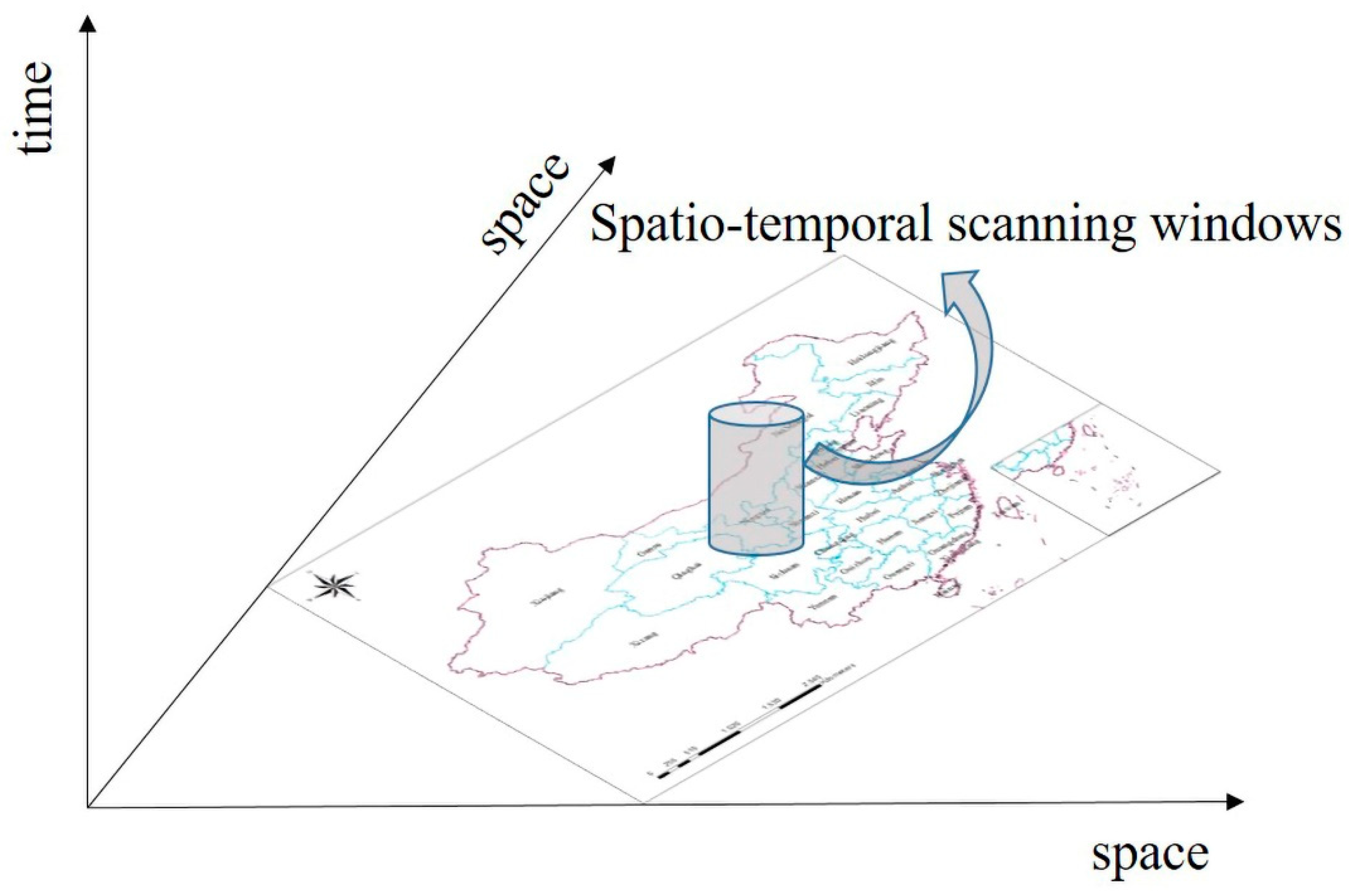
2.3. Spatio-Temporal Scanning Model

STSM selects an event in the scanning area as the center of the bottom surface of the dynamic cylinder scanning window, continuously enlarging the radius of the bottom surface (the upper limit of the radius is generally set less than or equal to 50% of the total number of points in the research area) and the height of the cylinder (the upper limit of the time is generally set greater than or equal to 50% of the maximum time sequence) until reaching the upper limit. This scanning process will repeat for each event in study area (Figure 1). Then, the LLR and RR are calculated based on the actual number of events and expected number of events inside and outside the scanning window. Finally, the sample data of the scanning area are simulated multiple times using the Monte Carlo randomization method to obtain a confidence value of the aggregated regions. The window of the spatio-temporal clustering area needs to satisfy both the LLR greater than 0 (LLR > 0) and the ratio of extreme precipitation events in the window greater than outside (RR > 1). Among all the clustering areas, the clustering area with the maximum LLR is the first-level accumulation area, indicating that the clustering area has the highest occurrence probability of extreme precipitation.
There are only two states for the daily precipitation extreme precipitation event data (either extreme or not extreme precipitation events), which are suitable for the Bernoulli distribution model, also known as a typical 0–1 distribution. Both the shape and size of the scanning windows should be considered: based on the structure of the scanning regions and the spatial characteristics of China, we adopted a circular scanning window. The principle of the STSM is as followed:
The probability of extreme precipitation events (P) for the entire study area G can be calculated by Equation (1), where m z is the actual number of extreme precipitation events in the scanning window Z, μ ( Z ) is the total number of events, μ ( G ) is the total number of extreme precipitation events in all regions G, m s is the actual number of extreme precipitation events, p [ 0 , 1 ] is the probability of extreme precipitation events in the scanning window, and q [ 0 , 1 ] is the probability of extreme precipitation events outside the scanning window.
P = p m z ( 1 - p ) μ ( Z ) - m z q m g - m z ( 1 - q ) ( ( μ ( G ) - μ ( Z ) ) - ( m g - m z )
Assuming L(Z) is the likelihood function value of the spatio-temporal scanning window Z, then Equation (1) can be expressed as Equation (2):
L ( Z ) = ( m z μ ( Z ) ) m z ( 1 - m z μ ( Z ) ) μ ( Z ) - m z ( m g - m z μ ( G ) - μ ( Z ) ) m g - m z ( 1 - m g - m z μ ( G ) - μ ( Z ) ) ( ( μ ( G ) - μ ( Z ) ) - ( m g - m z )
Based on the null assumption, the likelihood function L 0 is given as Equation (3):
L 0 = ( m g μ ( G ) ) m g ( μ ( G ) - m G μ ( G ) ) μ ( G ) - m g
K is an indication function. If the probability of an extreme precipitation event in the spatio-temporal scanning window is greater than the outside of the window, K = 1; otherwise, it is 0. The maximum LLR in Z has the expression in Equation (4):
max   LLR = maxlog [ L ( Z ) L 0 ] K ( m z μ z > m g - m z μ ( G ) - μ ( Z ) )
LLR is mainly used to characterize the probability of the spatio-temporal accumulation area; RR is mainly used to characterize the spatio-temporal persistence through measuring the number of extreme precipitation grids inside and outside the spatio-temporal clusters. RR is defined as Equation (5), where n i and E i represent the number of extreme precipitation events and the number of expected extreme precipitation events, observed in the spatio-temporal scanning window i, respectively; N represents the total number of extreme precipitation grids in the study area; E represents the total expected number of extreme precipitation grids in the study area. N is equal to E to meet the data requirements of the spatio-temporal scanning.
RR i = n i / E i ( N - n i ) / ( E - E i )
To ensure the results are statistically significant (p <= 0.001), this experiment randomly generates M data sets according to the Monte Carlo test.

2.4. Local Spatial Autocorrelation Model

Spatial autocorrelation is one of the most commonly used models for spatial aggregation [48,49]. It can measure the correlation of the same object in different spatial locations. Spatial autocorrelation is divided into global spatial autocorrelation and local spatial autocorrelation. The global spatial autocorrelation assumes that the space is homogeneous and one trend exists in the entire region. Its value is between −1.0 and 1.0 through normalization. Moran’s I > 0 indicates a positive spatial correlation in the spatial unit; the larger the value, the more aggregative the units. Moran’s I < 0 indicates a negative spatial correlation in the spatial unit; the smaller the value, the sparser the units. Moran’s I = 0 indicates that the spatial unit does not have spatial autocorrelation and is randomly distributed. However, it can only detect the global spatial aggregation, and cannot locate the specific accumulation area [50,51,52]. Therefore, it is necessary to introduce local spatial autocorrelation to analyse the local aggregation characteristics aggregation, such as LISA (local indicators of spatial association) and Moran’s I scatter plot.
LISA applies the Moran index to each regional unit, describing the similarities between the spatial units and its neighborhood. Moran scatter plots use a two-dimensional coordinate system to visually describe observed variables and spatial lag vectors. The x-axis represents the normalized observations, and the y-axis represents the spatial lag vector (the weighted average of the observations around the observation). The coordinate system is divided into four quadrants (HH, HL, LL, and LH) according to the order of the combination of high and low, which represent the spatial relationship between a certain research area and the adjacent area. Among them, the first quadrant indicates a high-value aggregation (HH), that the Moran index is positive, the z score is positive, and the LISA value is positive (aggregate). We chose Queen’s case as the spatial weight matrix with eight neighborhoods. At the same time, the LISA value is calculated according to Equation (6), where S is the cumulative precipitation difference, t i and t j are the precipitation at i and j, respectively, t is the mean precipitation, and Z ( I i ) obeys the standard normal distribution. Z ( I i ) is calculated by normalizing the local autocorrelation index I i to obtain the significance p of each grid point. This paper considers p-values that do not exceed 0.001 to be statistically significant.
S = { 1 n i = 1 n ( t i t ) ,   t i t 0 ,   t i < t ; I i = ( t i t ¯ ) S j = 1 n w i ,   j j = 1 n w i ,   j ( t j t ¯ ) ; Z ( I i ) = I - E [ I i ] V [ I i ] ;

2.5. Experimental Process

The main experimental steps in this paper are shown in Figure 2: first, the extreme precipitation threshold based on the daily precipitation grid data from 1979 to 2018 by percentile threshold method was extracted using the 31 × 40 time sliding window. Then, the extreme precipitation threshold and daily precipitation value were compared to select the extreme precipitation grid. Second, the spatio-temporal clusters of extreme precipitation in July 2016 were extracted using the Bernoulli distribution’s STSM. Third, the LSAM was used to detect the hot spots with accumulated precipitation differences to achieve fine positioning. Finally, the extracted spatio-temporal clusters of extreme precipitation were compared with the historical extreme precipitation events to evaluate the extraction accuracy of the STSM.

3. Results

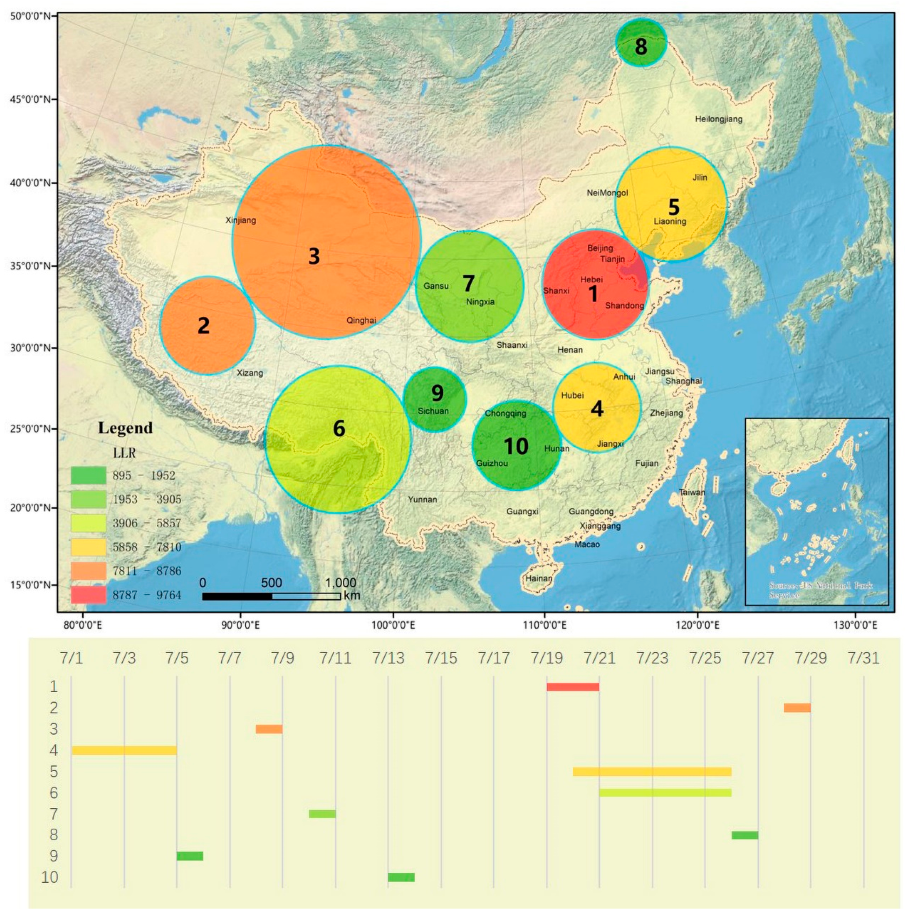
3.1. Spatio-Temporal Aggregation Characteristics of Extreme Precipitation Events

When using STSM, the parameters have a great influence on the results. In this paper, we set the spatial scanning window threshold parameter to 5%, 10%, 15%, and 20%, then applied them to extract the spatio-temporal clusters of extreme precipitation events in China July 2016.
As Figure 3 shows, when the spatial scanning window parameter is set to 5%, the scanning result is too fragmented. Almost the whole of China has accumulation areas, and many accumulation areas are small and dense, which cannot effectively represent the spatio-temporal aggregation of extreme precipitation events. When the parameter is set to 10%, the accumulation area starts to have a good degree of discrimination, but the number of accumulation areas is still too high. When the spatial scanning window is set to 15% and 20%, the positions and sizes of the extreme precipitation accumulation areas tend to be similar. Although the accumulation areas of 20% coincides with the accumulation areas of 15%, and both show obvious spatio-temporal aggregation characteristics; the number of accumulation areas are reduced when the parameter is set to 20%, which are relatively rough, overlooking small areas with extreme precipitation, and may include spurious accumulation areas where extreme precipitation events did not exist. The spatial scan window parameter is better set to 15% (an appropriate level of detail and better consistency) with the advantage of a stable calculation result. The time scan window parameter is set to an empirical value of 50% [53]. The results of the 15% scanning window are shown in Table 1 and Figure 4.
The STSM detected ten statistically significant (through confidence tests) spatio-temporal clusters, which better reflected the distribution of extreme precipitation events in time and space (Figure 4). Cluster 1 is centered on 37.95 N, 115.65 E with a radius of 393.84 km. From the provincial perspective, it is mainly centered on Hebei, Shanxi, Shandong and Henan. The accumulation lasted two days from 19 July to 20 July. Its corresponding LLR is 9763.16, which is 1.13 times the aggregation degree of cluster 2. It’s RR also reaches the third highest value (8.69). Cluster 2 centered on 33.95 N, 83.95 E with a radius of 350.26 km, covering the northern Xizang and southern Xinjiang, with the highest RR (12.52). Cluster 8 reaches the second highest value (11.69). Other statistically significant clusters (p < 0.001) have relatively small RR values that gradually reduce with a more stable gradient. Cluster 6, 7, 8, 9, and 10′s LLR are relatively smaller than cluster 1, 2, 3, 4, 5. Cluster 5′s LLR is 1.7 times than cluster 6. The extreme precipitation duration is short, and the detected clusters over three days only include cluster 4, cluster 5, and cluster 6.

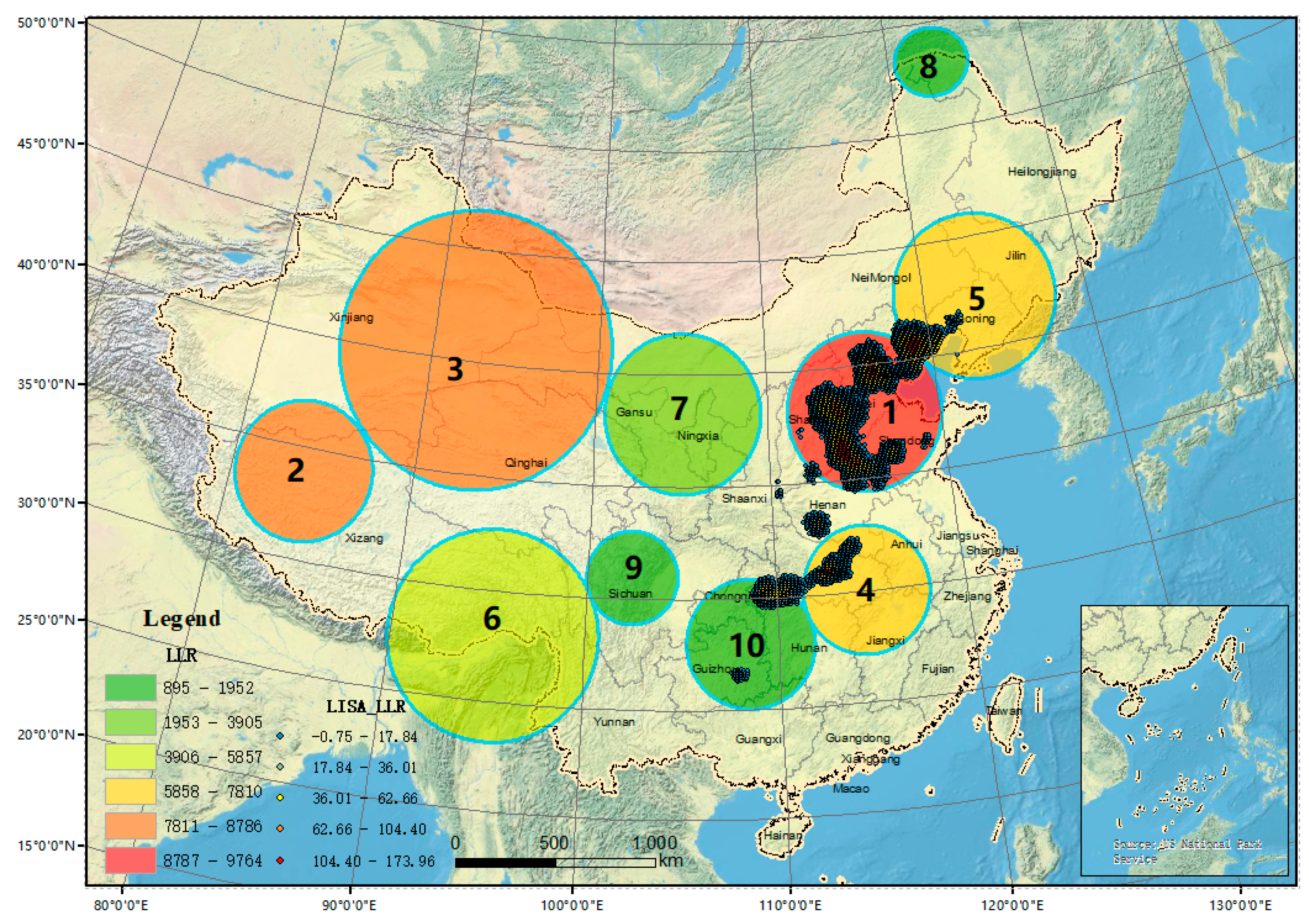
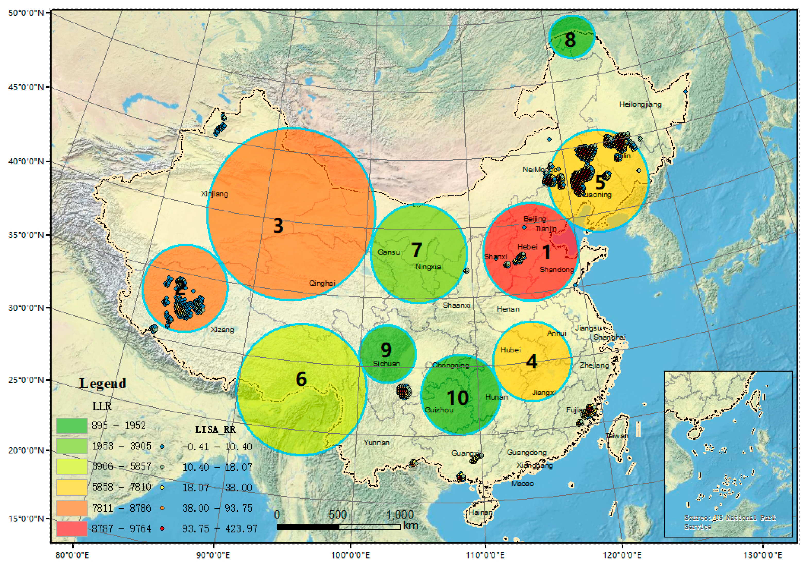
3.2. Internal Spatio-Temporal Aggregation Characteristics with the Local Spatial Autocorrelation Model

Combined with the LSAM to further explore the internal aggregation characteristics of the spatio-temporal accumulation area of extreme precipitation, we selected the largest LLR (cluster 1) and largest RR (cluster 8) as examples. The difference between the daily maximum precipitation value and the extreme precipitation threshold was accumulated, then hot spots in the extreme precipitation areas were extracted by GeoDa. Cluster 1 starts from 19 July 2016 to 20 July 2016, lasting for two days. The Moran’s I scatter plot (left) and p-values (right) in space are shown in Figure 5.
China’s cumulative precipitation difference from 19 to 20 July 2016 has a significant correlation. Moran’s I correlation index reaches 0.984636. The high-high value regions (extreme precipitation events surrounded by extreme precipitation events) are mainly distributed in Hebei, Shanxi, Henan, Hubei.
By overlapping the high-high value regions (p > 0.001) and the spatio-temporal clusters in Figure 4, we found that cluster 1 had obvious hotspots; cluster 4, cluster 5, and cluster 10 also had some hotspots (Figure 6). They decreased outwards from one of the internal regions, surrounded by low-value regions. The possible reason for this distribution is that the cumulative precipitation difference is selected from 19 July 2016, to 20 July 2016, where extreme precipitation events occurred in these regions; other regions of China are more stable. These results suggest that the combined use of LSAM is helpful for the exploration of the internal aggregation characteristics of these clusters.
China’s cumulative precipitation difference on 28 July 2016 also has a significant correlation (Figure 7). Moran’s I correlation index reaches 0.91667, slightly smaller than the highest LLRs Moran’s I, perhaps because of sparser precipitation. The high-high values are mainly distributed in cluster 2, cluster 5 and cluster 1, which occurred near 28 July 2016 (Figure 8). In addition, the LISA value on 28 July 2016, which reached 423.97, is larger than the LISA value on 19 to 20 July 2016, which reached 173.96. This indicates that RR is more suitable for characterizing the actual spatio-temporal persistence of the accumulation areas, which is also more catastrophic; LLR is more suitable for characterizing the most likely spatio-temporal accumulation areas. Although the region with a larger RR has a higher probability of occurrence (LLR) of extreme precipitation events, there is no clear positive correlation; that is, the region most likely to have extreme precipitation events does not necessarily have the strongest RR, and the assessment of catastrophic ability must consider the local natural environment.
Taken together, these results suggest that extreme precipitation events are more likely to occur in eastern and northern China with a significant aggregation, e.g., North China Plain centered on Hebei, north-western China centered on Gansu, and the Tianshan Mountains.

4. Discussion

Our research, coupled the spatial and temporal properties of extreme precipitation events using STSM, successfully discovered the spatio-temporal clusters of extreme precipitation events. To optimize the spatial positions of the extreme precipitation events, LSAM was used to further detect the internal distribution of extreme precipitation clusters. According to the meteorological reports provided by the National Information Centre, extreme precipitation in 2016 was mainly concentrated in East China and North China, and the North China Plain is the rainstorm center far beyond the same period of national precipitation from 18 to 20 July 2016 [54,55]. Zhou et al. used 2016 rainwater and typhoon information collected by the Water Resources and Hydrology Bureau of China to analyze the extreme precipitation events, finding that the extreme precipitation process began early, was long lasting, and widely covered China in 2016 [56]. Twenty-eight provinces and cities were influenced by these extreme precipitation events: the first echelon affected by extreme precipitation events were along the Yangtze river: Jiangxi, Hunan, Zhejiang, Guangdong, and Fujian; the second echelon (Guangxi, Shanghai, Anhui, Chongqing, Hubei, Jiangsu, and Guizhou) was basically located on the outskirts of the first echelon [56]. They are highly coincident with economically developed regions, causing a major impact on China’s economic development. Extreme precipitation events have also occurred in the inland areas, e.g., Xinjiang and Gansu corresponded to cluster 2 and cluster 3. These studies are highly consistent with our findings, which showed that STSM combined with LSAM is useful in recognizing the aggregation characteristics of extreme precipitation events. Particularly, this method contributes to a decrease in subjective and an increase in objective information when determining the location and range of extreme precipitation areas through coupling the spatial and temporal scale, and enables the quantitative evaluation of these areas with LLR and RR.
There are also some limitations in this study. First, although the percentile threshold method can reduce the influence of spatio-temporal heterogeneity and climate multi-deformation, it cannot eliminate the influence of the threshold divided subjectivity by human. Second, the spatial resolution (0.1° × 0.1°) and time scale (d) of the China Meteorological Forcing Data are still rough. The extraction accuracy of extreme precipitation events is insufficient. Third, the fixed window shape of the STSM limits the fine-grained extraction of spatio-temporal clusters; thus, it is easy to obtain false spatio-temporal clusters. Finally, the RR can reflect the spatio-temporal persistence of the clusters of extreme precipitation, but it cannot indicate the concentration degrees of different intensities or frequencies. It is necessary to improve the quantitative description index. If more refined data and more accurate models can be used, the detection of spatio-temporal clusters of extreme precipitation events will have more practical significance.

5. Conclusions

In this study, we coupled the spatial extent and the temporal range of extreme precipitation events to analyze the spatio-temporal aggregation characteristics by using the STSM (spatio-temporal scanning model) and LSAM (local spatial autocorrelation model), then applied this method to China. Through the STSM’s dynamic scanning window, the spatio-temporal clusters break the limitation of subjective divisions, better synthesizing the temporal and spatial properties of extreme precipitation with an unbiased result. Combined with LSAM, we can detect the precise location of extreme precipitation in spatio-temporal clusters. The result showed that China’s summer extreme precipitation events in 2016 are significantly aggregated. The clusters of extreme precipitation events are mainly distributed in eastern and northern China, such as cluster 1 located on Hebei, cluster 2 and cluster 3 located around Xinjiang, cluster 4 located on the middle basin of the Yangtze River and Xinjiang.
The LLR and RR in STSM are important quantitative evaluation indicators, which are not only helpful detect the location of extreme precipitation, but also for the quantitative evaluation of the aggregation degree. Although the clusters of extreme precipitation events with a larger RR also have a larger LLR, there is no obvious positive correlation among them. RR is more representable to catastrophic extreme precipitation.

Author Contributions

Conceptualization, S.Y. and C.C.; methodology, C.W. and T.Z.; software, C.W.; validation, C.W.; formal analysis, C.W., S.S. and T.Z.; investigation, S.S.; resources, S.Y.; data curation, S.Y.; writing—original draft preparation, C.W. and S.Y.; writing—review and editing, C.W. and S.Y.; visualization, C.W.; supervision, S.Y.; project administration, S.Y.; funding acquisition, C.C. All authors have read and agreed to the published version of the manuscript.

Funding

This work was supported by National Key Research and Development Plan of China [grant numbers No.2019YFA0606901]; National Natural Science Foundation of China [grant number 41801300, 41901316].

Acknowledgments

We would like to thank the high-performance computing support from the Center for Geodata and Analysis, Faculty of Geographical Science, Beijing Normal University [https://gda.bnu.edu.cn/]. We thank Chiyuan Miao for helpful discussion.

Conflicts of Interest

The authors declare no conflict of interest.

References

  1. Tammets, T.; Jaagus, J. Climatology of precipitation extremes in Estonia using the method of moving precipitation totals. Theor. Appl. Climatol. 2013, 111, 623–639. [Google Scholar] [CrossRef]
  2. Zhang, Q.; Zhou, Y.; Singh, V.P.; Li, J. Scaling and clustering effects of extreme precipitation distributions. J. Hydrol. 2012, 454, 187–194. [Google Scholar] [CrossRef]
  3. Shukla, R.; Agarwal, A.; Sachdeva, K.; Kurths, J.; Joshi, P.K. Climate change perception: An analysis of climate change and risk perceptions among farmer types of Indian Western Himalayas. Clim. Chang. 2019, 152, 103–119. [Google Scholar] [CrossRef]
  4. Alexander, L.V.; Zhang, X.; Peterson, T.C.; Caesar, J.; Gleason, B.; Klein Tank, A.M.G.; Tagipour, A. Global observed changes in daily climate extremes of temperature and precipitation. J. Geophys. Res. Atmos. 2006, 111, 5. [Google Scholar] [CrossRef] [Green Version]
  5. Allan, R.P.; Soden, B.J. Atmospheric warming and the amplification of precipitation extremes. Science 2008, 321, 1481–1484. [Google Scholar] [CrossRef] [PubMed] [Green Version]
  6. Gao, T.; Xie, L. Study on progress of the trends and physical causes of extreme precipitation in China during the last 50 years. Adv. Earth Sci. 2014, 29, 577–589. [Google Scholar]
  7. IPCC Climate Change. The Physical Science Basis. Working Group I Contribution to the Fifth Assessment Report of the Intergovernmental Panel on Climate Change; Cambridge University Press: Cambridge, UK, 2013. [Google Scholar]
  8. Dai, A.; Trenberth, K.E.; Karl, T.R. Global variations in droughts and wet spells: 1900–1995. Geophys. Res. Lett. 1998, 25, 3367–3370. [Google Scholar] [CrossRef] [Green Version]
  9. Goswami, B.N.; Venugopal, V.; Sengupta, D.; Madhusoodanan, M.S.; Xavier, P.K. Increasing trend of extreme rain events over India in a warming environment. Science 2006, 314, 1442–1445. [Google Scholar] [CrossRef] [Green Version]
  10. Liu, B.; Chen, J.; Chen, X.; Lian, Y.; Wu, L. Uncertainty in determining extreme precipitation thresholds. J. Hydrol. 2013, 503, 233–245. [Google Scholar] [CrossRef]
  11. Min, S.; Qian, Y.F. Regionality and persistence of extreme precipitation events in China. Adv. Water Sci. 2008, 19, 763–771. [Google Scholar]
  12. Yang, P. Research of Group-occurring Extreme Temperature and Precipitation Events during 1960–2005. Ph.D. Thesis, Lanzhou University, Lanzhou, China, 2009. [Google Scholar]
  13. Cheung, K.K.; Ozturk, U. Synchronization of extreme rainfall during the Australian summer monsoon: Complex network perspectives. Chaos Interdiscip. J. Nonlinear Sci. 2020, 30, 063117. [Google Scholar] [CrossRef] [PubMed]
  14. Kunkel, K.E.; Easterling, D.R.; Redmond, K.; Hubbard, K. Temporal variations of extreme precipitation events in the United States: 1895–2000. Geophys. Res. Lett. 2003, 30, 17. [Google Scholar] [CrossRef] [Green Version]
  15. Groisman, P.Y.; Knight, R.W.; Easterling, D.R.; Karl, T.R.; Hegerl, G.C.; Razuvaev, V.N. Trends in intense precipitation in the climate record. J. Clim. 2005, 18, 1326–1350. [Google Scholar] [CrossRef]
  16. Ren, F.; Cui, D.; Gong, Z.; Wang, Y.; Zou, X.; Li, Y.; Wang, X. An objective identification technique for regional extreme events. J. Clim. 2012, 25, 7015–7027. [Google Scholar] [CrossRef]
  17. Easterling, D.R.; Evans, J.L.; Groisman, P.Y.; Karl, T.R.; Kunkel, K.E.; Ambenje, P. Observed variability and trends in extreme climate events: A brief review. Bull. Am. Meteorol. Soc. 2000, 81, 417–426. [Google Scholar] [CrossRef] [Green Version]
  18. Biondi, F.; Kozubowski, T.J.; Panorska, A.K. Stochastic modeling of regime shifts. Clim. Res. 2002, 23, 23–30. [Google Scholar] [CrossRef]
  19. Biondi, F.; Kozubowski, T.J.; Panorska, A.K.; Saito, L. A new stochastic model of episode peak and duration for eco-hydro-climatic applications. Ecol. Model. 2008, 211, 383–395. [Google Scholar] [CrossRef]
  20. Blanchet, J.; Ceresetti, D.; Molinié, G.; Creutin, J.D. A regional GEV scale-invariant framework for Intensity–Duration–Frequency analysis. J. Hydrol. 2016, 540, 82–95. [Google Scholar] [CrossRef]
  21. Gentilucci, M.; Barbieri, M.; Lee, H.S.; Zardi, D. Analysis of rainfall trends and extreme precipitation in the Middle Adriatic Side, Marche Region (Central Italy). Water 2019, 11, 1948. [Google Scholar] [CrossRef] [Green Version]
  22. Jing, C.; Jiang, T.; Wang, Y.J.; Chen, J.; Jian, D.; Luo, L.; Buda, S.U. A study on regional extreme precipitation events and the exposure of population and economy in China. Acta Meteor. Sin. 2016, 74, 572–582. [Google Scholar]
  23. Andreadis, K.M.; Clark, E.A.; Wood, A.W.; Hamlet, A.F.; Lettenmaier, D.P. Twentieth-century drought in the conterminous United States. J. Hydrometeorol. 2005, 6, 985–1001. [Google Scholar] [CrossRef]
  24. Yuan, N.; Fu, Z.; Mao, J. Different scaling behaviors in daily temperature records over China. Phys. A Stat. Mech. Appl. 2010, 389, 4087–4095. [Google Scholar] [CrossRef]
  25. Chen, Y.; Zhai, P. Persistent extreme precipitation events in China during 1951–2010. Clim. Res. 2013, 57, 143–155. [Google Scholar] [CrossRef] [Green Version]
  26. Ghosh, S.; Mallick, B.K. A hierarchical Bayesian spatio-temporal model for extreme precipitation events. Environmetrics 2011, 22, 192–204. [Google Scholar] [CrossRef]
  27. Zhang, Q.; Singh, V.P.; Li, J.; Jiang, F.; Bai, Y. Spatio-temporal variations of precipitation extremes in Xinjiang, China. J. Hydrol. 2012, 434, 7–18. [Google Scholar] [CrossRef]
  28. Agarwal, A. Unraveling Spatio-Temporal Climatic Patterns via Multi-Scale Complex Networks. Ph.D. Thesis, Universität Potsdam, Potsdam, Germany, 2019. [Google Scholar]
  29. Naus, J.I. The distribution of the size of the maximum cluster of points on a line. J. Am. Stat. Assoc. 1965, 60, 532–538. [Google Scholar] [CrossRef]
  30. Kulldorff, M.; Nagarwalla, N. Spatial disease clusters: Detection and inference. Stat. Med. 1995, 14, 799–810. [Google Scholar] [CrossRef]
  31. Kulldorff, M.; Athas, W.F.; Feurer, E.J.; Miller, B.A.; Key, C.R. Evaluating cluster alarms: A space-time scan statistic and brain cancer in Los Alamos, New Mexico. Am. J. Public Health 1998, 88, 1377–1380. [Google Scholar] [CrossRef] [Green Version]
  32. Kim, Y.; O’Kelly, M. A bootstrap based space–time surveillance model with an application to crime occurrences. J. Geogr. Syst. 2008, 10, 141–165. [Google Scholar] [CrossRef]
  33. Horn, L.M. Precipitation Associated with Increased Diarrheal Disease in Mozambique; A Time Series Analysis. Ph.D. Thesis, University of Washington, Washington, DC, USA, 2017. [Google Scholar]
  34. Ye, S.J.; Lu, S.H.; Bai, X.S.; Gu, J.F. ResNet-Locust-BN network-based automatic identification of east asian migratory locust species and instars from RGB images. Insects 2020, 11, 458. [Google Scholar] [CrossRef] [PubMed]
  35. Gong, D.Y.; Wang, S.W. Severe summer rainfall in China associated with enhanced global warming. Clim. Res. 2000, 16, 51–59. [Google Scholar] [CrossRef]
  36. Yao, C.; Yang, S.; Qian, W.; Lin, Z.; Wen, M. Regional summer precipitation events in Asia and their changes in the past decades. J. Geophys. Res. Atmos. 2008, 113, 17. [Google Scholar] [CrossRef] [Green Version]
  37. Sun, Q.H.; Miao, C.Y.; Duan, Q.Y. Changes in the Spatial Heterogeneity and Annual Distribution of Observed Precipitation across China. J. Clim. 2017, 30, 9399–9416. [Google Scholar] [CrossRef]
  38. Miao, C.Y.; Duan, Q.Y.; Sun, Q.H.; Lei, X.H.; Li, H. Non-uniform changes in different categories of precipitation intensity across China and the associated large-scale circulations. Environ. Res. Lett. 2019, 14. [Google Scholar] [CrossRef]
  39. Xie, P.; Janowiak, J.E.; Arkin, P.A.; Adler, R.; Gruber, A.; Ferraro, R.; Curtis, S. GPCP pentad precipitation analyses: An experimental dataset based on gauge observations and satellite estimates. J. Clim. 2003, 16, 2197–2214. [Google Scholar] [CrossRef] [Green Version]
  40. Higgins, R.W.; Silva, V.B.S.; Shi, W.; Larson, J. Relationships between climate variability and fluctuations in daily precipitation over the United States. J. Clim. 2007, 20, 3561–3579. [Google Scholar] [CrossRef]
  41. Ye, S.J.; Zhu, D.H.; Yao, X.C.; Zhang, N.; Fang, S.; Li, L. Development of a Highly Flexible Mobile GIS-Based System for Collecting Arable Land Quality Data. IEEE J. Sel. Top. Appl. Earth Obs. Remote Sens. 2014, 5, 14. [Google Scholar] [CrossRef]
  42. Yatagai, A.; Arakawa, O.; Kamiguchi, K.; Kawamoto, H.; Nodzu, M.I.; Hamada, A. A 44-year daily gridded precipitation dataset for Asia based on a dense network of rain gauges. Sola 2009, 5, 137–140. [Google Scholar] [CrossRef] [Green Version]
  43. Yang, K. China Meteorological Forcing Data (1979–2018). Nat. Tibet. Plateau Data Cent. 2018. [Google Scholar] [CrossRef]
  44. Yang, K.; He, J.; Tang, W.; Qin, J.; Cheng, C.C. On downward shortwave and longwave radiations over high altitude regions: Observation and modeling in the Tibetan Plateau. Agric. Forest Meteorol. 2010, 150, 38–46. [Google Scholar] [CrossRef]
  45. He, J.; Yang, K.; Tang, W.; Lu, H.; Qin, J.; Chen, Y.; Li, X. The first high-resolution meteorological forcing dataset for land process studies over China. Sci. Data 2020, 7, 1–11. [Google Scholar] [CrossRef] [Green Version]
  46. Ye, S.J.; Yan, T.L.; Yue, Y.-L.; Lin, W.-Y.; Li, L.; Yao, X.-C.; Mu, Q.-Y.; Li, Y.-Q.; Zhu, D. Developing a reversible rapid coordinate transformation model for the cylindrical projection. Comput. Geosci. 2016, 89, 44–56. [Google Scholar] [CrossRef]
  47. Ye, S.; Liu, D.; Yao, X.; Tang, H.; Xiong, Q.; Zhuo, W.; Du, Z.; Huang, J.; Su, W.; Shen, S.; et al. RDCRMG: A Raster Dataset Clean & Reconstitution Multi-Grid Architecture for Remote Sensing Monitoring of Vegetation Dryness. Remote Sens. 2018, 10, 1376. [Google Scholar] [CrossRef] [Green Version]
  48. Sokal, R.R.; Thomson, J.D. Applications of spatial autocorrelation in ecology. In Develoments in Numerical Ecology; Springer: Berlin/Heidelberg, Germany, 1987; pp. 431–466. [Google Scholar]
  49. Ord, J.K.; Getis, A. Testing for local spatial autocorrelation in the presence of global autocorrelation. J. Reg. Sci. 2001, 41, 411–432. [Google Scholar] [CrossRef]
  50. Wang, P.A.; Luo, W.H.; Bai, Y.P. Comparative analysis of aggregation detection based on spatial autocorrelation and spatial-temporal scan statistics. Hum. Geogr. 2012, 27, 119–127. [Google Scholar]
  51. Ye, S.J.; Song, C.Q.; Shen, S.; Gao, P.C.; Cheng, C.X.; Cheng, F.; Wan, C.J.; Zhu, D.H. Spatial pattern of arable land-use intensity in China. Land Use Policy 2020, 99, 104845. [Google Scholar] [CrossRef]
  52. Ye, S.J.; Cheng, C.X.; Song, C.Q.; Shen, S. Visualizing bivariate local spatial autocorrelation between commodity revealed comparative advantage index of China and USA from a new space perspective. Environ. Plan. A Econ. Space 2020, 9. [Google Scholar] [CrossRef]
  53. Sherman, R.L.; Henry, K.A.; Tannenbaum, S.L.; Feaster, D.J.; Kobetz, E.; Lee, D.J. Peer reviewed: Applying spatial analysis tools in public health: An example using SaTScan to detect geographic targets for colorectal cancer screening interventions. Prev. Chronic Dis. 2014, 11, E41. [Google Scholar] [CrossRef] [PubMed] [Green Version]
  54. BI, B.; Zhang, X.; Dai, K. Characteristics of 2016 severe convective weather and extreme rainfalls under the background of super El Niño. Chin. Sci. Bull. 2017, 62, 928–937. [Google Scholar] [CrossRef] [Green Version]
  55. Gao, R.; Song, L.C.; Zhong, H.L. Characteristics of extreme precipitation in China during the 2016 flood season and comparison with the 1998 situation. Meteor Mon. 2018, 44, 699–703. [Google Scholar]
  56. Zhou, G.L.; Gao, W.Q.; Huang, C.X. Analysis of the extreme rainstorm events in China in 2016. China Flood Control Drought Relief 2017, 27, 75. (In Chinese) [Google Scholar]
Figure 1. Schematic diagram of the spatio-temporal scanning model (STSM).
Atmosphere 12 00218 g001
Figure 2. Spatio-temporal aggregation detection flow chart for extreme precipitation. LLR: log likelihood ratio; RR: relative risk; LISA: local indicators of spatial association.
Atmosphere 12 00218 g002
Figure 3. The results for scanning window thresholds set to 5%, 10%, 15%, and 20%.
Atmosphere 12 00218 g003
Figure 4. Spatio-temporal aggregation pattern of extreme precipitation events in July 2016, China.
Atmosphere 12 00218 g004
Figure 5. Moran’s I scatter plot (left) and p-values (right) in China from 19 to 20 July 2016.
Atmosphere 12 00218 g005
Figure 6. Overlap between the high–high value areas and the clusters of the STSM from 19 to 20 July 2016.
Atmosphere 12 00218 g006
Figure 7. Moran’s I scatter plot (left) and p-values (right) in China on 28 July 2016.
Atmosphere 12 00218 g007
Figure 8. Overlap between the high–high value areas and the clusters of the STSM on 28 July 2016.
Atmosphere 12 00218 g008
Table 1. Spatio–temporal scan results of China from 1 to 31 July 2016 (15%).
Cluster DateCluster RegionNumber of EventsExpected EventsLog Likelihood RatioRelative Riskp-Value
2016/07/19–2016/07/2016000707.019763.168.690.001
2016/07/28–2016/07/2823598287.498634.2912.700.001
2016/07/08–2016/07/08367031079.898130.936.360.001
2016/07/01–2016/07/0445819931.857091.636.380.001
2016/07/20–2016/07/25588742201.446724.744.150.001
2016/07/21–2016/07/25665051903.843937.853.490.001
2016/07/10–2016/07/1072474390.883041.106.390.001
2016/07/26–2016/07/26867757.901493.5311.730.001
2016/07/05–2016/07/059879122.001221.127.230.001
2016/07/13–2016/07/13101047232.35895.074.520.001
Publisher’s Note: MDPI stays neutral with regard to jurisdictional claims in published maps and institutional affiliations.

