Air Concentrations of Gaseous Elemental Mercury and Vegetation–Air Fluxes within Saltmarshes of the Tagus Estuary, Portugal

Abstract

In situ air concentrations of gaseous elemental mercury (Hg(0)) and vegetation–atmosphere fluxes were quantified in both high (Cala Norte, CN) and low-to-moderate (Alcochete, ALC) Hg-contaminated saltmarsh areas of the Tagus estuary colonized by plant species Halimione portulacoides (Hp) and Sarcocornia fruticosa (Sf). Atmospheric Hg(0) ranged between 1.08–18.15 ng m⁻³ in CN and 1.18–3.53 ng m⁻³ in ALC. In CN, most of the high Hg(0) levels occurred during nighttime, while the opposite was observed at ALC, suggesting that photoreduction was not driving the air Hg(0) concentrations at the contaminated site. Vegetation–air Hg(0) fluxes were low in ALC and ranged from −0.76 to 1.52 ng m⁻² (leaf area) h⁻¹ for Hp and from −0.40 to 1.28 ng m⁻² (leaf area) h⁻¹ for Sf. In CN, higher Hg fluxes were observed for both plants, ranging from −9.90 to 15.45 ng m⁻² (leaf area) h⁻¹ for Hp and from −8.93 to 12.58 ng m⁻² (leaf area) h⁻¹ for Sf. Mercury flux results at CN were considered less reliable due to large and fast variations in the ambient air concentrations of Hg(0), which may have been influenced by emissions from the nearby chlor-alkali plant, or historical contamination. Improved experimental setup, the influence of high local Hg concentrations and the seasonal activity of the plants must be considered when assessing vegetation–air Hg(0) fluxes in Hg-contaminated areas.

1. Introduction

Mercury (Hg) is a naturally occurring and toxic metal that is present in natural ecosystems. Gaseous elemental mercury (Hg(0)) is the dominant form of natural and anthropogenic Hg emissions, comprising >95% of the total Hg in air [1]. It has an atmospheric lifetime of 0.8–1.7 years after emission [2], resulting in long-range transport through the atmosphere [3]. In addition to primary anthropogenic emissions, Hg is re-emitted as Hg(0) from land and ocean surfaces to the atmosphere after reduction of Hg(II) pools in terrestrial and aquatic ecosystems [4,5]. Measuring and modeling of Hg emissions from representative surfaces are crucial to evaluate the role of natural terrestrial and aquatic environments on the cycling of Hg on both regional and global scales [6,7,8,9,10]. Aquatic ecosystems, especially wetlands, are key environments for Hg biogeochemical transformation and cycling [11,12]. Mercury air–surface gas exchange is an important but poorly characterized route for Hg transfer into or out of wetlands. In aquatic systems, Hg can be bioaccumulated throughout the food chain as methylmercury (a highly toxic organic Hg compound), or can be released back to the atmosphere as Hg(0) [13,14]. Since anthropogenic atmospheric Hg(0) can be recycled through and re-emitted from vegetation, it remains unclear if the biosphere is a long-term source or sink of Hg. Once nearly 30% of the earth’s land surface area is covered by vegetation (approximately 4 × 10⁹ ha) [15], it is crucial to quantify the role of vegetation in Hg emissions, on both regional and global scales, in order to develop accurate mass balances for global movements [16,17].

Air–surface Hg(0) fluxes are largely influenced by climate, substrate Hg concentration, soil chemistry, microbiology, sunlight, temperature, atmospheric turbulence, relative humidity, rain events, and vegetation cover [18,19]. The reduction of Hg(II) to Hg(0) catalyzed by solar radiation is also an important factor in both terrestrial [20] and aquatic [21] environments. The effect of vegetation on Hg biogeochemical cycling has been examined in terrestrial species [6,22,23,24]. Plant species, air Hg(0), and soil Hg concentrations have all been shown to influence vegetation–air Hg exchange, and terrestrial plants may act as either a source or sink for atmospheric Hg. Additionally, measurements of Hg(0) by dynamic flux chambers over marsh plants have shown bidirectional fluxes in a moderately Hg-contaminated estuary [10] and in pristine wetlands [25]. Several studies have shown that at ambient atmospheric Hg(0) concentrations (~1.5 ng m⁻³), vegetated terrestrial surfaces are net sinks of Hg(0), which is incorporated into leaf tissue in forests [26], grasslands [27], peatlands [28], or in the arctic tundra [29]. However, Hg land-atmosphere exchange in peatland environments not only shows uptake of Hg by vegetation but also re-emission of Hg(0) induced by photochemical processes at the peat surface and non-photochemical abiotic reduction by natural organic matter [30,31]. In fact, in over-barren, litter-covered, and vegetated soils, the Hg(0) flux, on average, switches from net deposition to net emission below an atmospheric Hg(0) concentration of 2.75 ng m⁻³ [32]. Nevertheless, in coastal wetlands, particularly in saltmarshes, measurements of Hg(0) flux from vegetation are still scarce [10,17,25,33,34] once these environments are difficult to operate, mostly the trace metal flux systems, due to a constantly changing environment.

Coastal wetlands are challenging ecosystems for gas exchange studies. In addition to the usual microclimatic variables (temperature, humidity, solar radiation, turbulence, air stability), variations in the redox potential and salinity due to regular tidal flooding and the role of plants in various stages of growth [35] are among several variables possibly influencing Hg(0) exchange. The formation of dissolved gaseous mercury (DGM) and Hg(0) volatilization in intertidal sediments can act as a potential source of Hg(0) to the atmosphere [36]. It has also been demonstrated that saltmarsh plants are potential sources of Hg(0) to the atmosphere [33] by taking up Hg from the roots and exporting it as Hg(0) through the leaves. Moreover, it has been established that the halophyte plant Halimione portulacoides can act as a bioindicator of Hg contamination in saltmarsh ecosystems [37]. However, there are limited studies examining the role of dominant emergent halophytes in Hg(0) flux. Measuring vegetation–air Hg(0) fluxes in the Tagus estuary, Canário et al. [10] stated that vegetation–air Hg(0) was light dependent, with the highest average daytime emission of 0.48 ± 0.40 ng Hg m⁻² h⁻¹ from H. portulacoides. Nevertheless, air Hg(0) contribution from aquatic vegetation in highly contaminated industrial areas remains poorly understood.

This study contributes to the knowledge of Hg dynamics in saltmarsh areas under natural and industry-impacted environments. We hypothesized that air Hg(0) concentrations in saltmarsh areas would be a result of mercury volatilization from both the intertidal sediment surface and stomatal evapotranspiration from vegetation. The objectives of this research were (1) to quantify Hg(0) in air concentrations and vegetation–air Hg(0) fluxes from saltmarsh areas with high and low-to moderate mercury contamination; (2) to compare total Hg concentrations (air, foliage, and surface sediment) between sites; and (3) to assess the significance of Hg(0) volatilization from saltmarsh vegetation in the mass balance of Hg in the Tagus estuary.

To achieve the presented main goals, the novelty of this study is the development of a specific experimental setup using dynamic flux chamber (DFC) methodology to assess air Hg(0) concentrations and vegetation–air Hg(0) fluxes in vegetated areas from two saltmarshes with distinct Hg impacts. The intercomparison of two distinct Hg-contaminated sites remains poorly described. In addition, the influence of different types of saltmarsh vegetation on air Hg(0) concentrations and vegetation–air Hg(0) fluxes are still ill-characterized. This study monitored a background area (ALC), inside a natural reserve, and a known Hg hotspot (CN) in the Tagus estuary. The obtained results allow us to understand how factors such as the developed experimental setup, the impact of high local Hg concentrations, and the vegetation type influence air Hg(0) concentrations and vegetation–air Hg(0) fluxes.

2. Materials and Methods

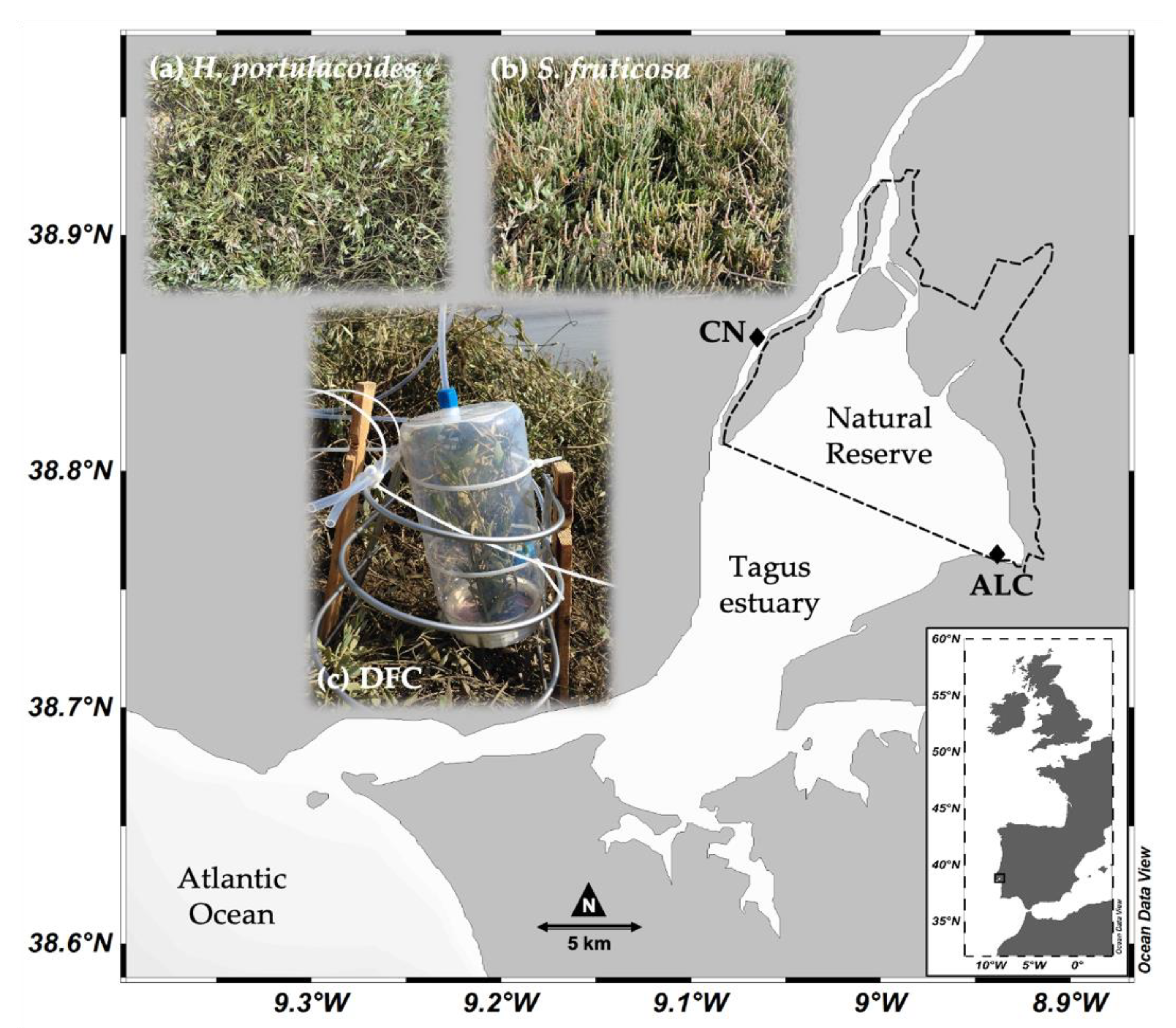
2.1. Site Description

The Tagus estuary is one of the most important wetland ecosystems in Europe, covering 325 km², of which 40% are intertidal areas (Figure 1).

It is a vertically well-mixed estuary with semi-diurnal mesotidal regime [38,39]. In the last decade, the mercury biogeochemical cycle has been widely studied in the Tagus estuary, focusing on the processes and fluxes of Hg in air [10,36], water [40,41], sediment, and biota [42,43,44,45,46]. The estuary in general is considered to be heavily Hg-contaminated mostly due to industrial pressures [47]. However, there is a significant protected area where mercury contamination is low to moderate [48]. The Tagus estuary margins (mainly the southern and eastern) contain extensive saltmarsh areas dominated by plant species such as the sea purslane (Halimione portulacoides), saltworth (Sarcocornia fruticosa), and small cordgrass (Spartina maritima), which cover ~95% of the colonized area.

For this study, two sampling areas in the Tagus estuary were chosen for the experimental setup according to their degree of Hg contamination (Figure 1). Cala Norte (CN) is located on the northern margin of the estuary (lat.: 38°51′21.2″ N; long.: 9°3′40.5″ W), approximately 50 m from a chlor-alkali plant and is considered a Hg hotspot [47]. In contrast, Alcochete (ALC) is located on the southern margin of the estuary (lat.: 38°45′40.2″ N; long.: 8°56′14.0″ W), inside a natural reserve (Ramsar area) without direct anthropogenic Hg impacts; therefore, having low to moderate Hg contamination [48].

2.2. Fieldwork

Vegetation–air Hg(0) fluxes and concentrations were measured continuously for four days in February 2018 at the regional background site in ALC saltmarsh and for four days in March 2018 at the mercury-impacted saltmarsh area CN using a dynamic flux chamber (DFC) method, modified from Zhang et al. [49]. Plant species Halimione portulacoides and Sarcocornia fruticosa were chosen to examine mercury flux patterns in relation to leaf surface area. In ALC, data collection started with the plant species H. portulacoides used to measure both air Hg(0) concentrations and fluxes, followed by the S. fruticosa plant species. In the CN site, the sampling occurred one month later, and the order of plant species used to obtain Hg(0) fluxes and concentrations data and the duration of measurements were similar to the ALC sampling site. Total mercury in aerial plant parts (stems and leaves) from each plant species and site, as well as in the corresponded sediments, were also determined.

2.3. Instrumentation and Analysis

2.3.1. Meteorological Parameters Measured In Situ

Meteorological parameters were monitored and recorded during the field studies. These included air temperature, solar radiation, wind speed, wind direction, and relative humidity, measured using a David Wireless Vantage Pro2 Plus meteorological station located near the flux chamber. Data logging was programmed to record data at 5 min intervals to match the analysis interval of the Hg measurements. In addition, soil surface temperature was also measured near surface at a depth of ~1 cm using HOBO node wireless sensors, from ONSET.

2.3.2. Atmospheric Mercury Analyzer

The Hg(0) concentrations were measured in situ using a Tekran 2537A mercury vapor analyzer (gold amalgamation thermo-desorption cold vapor atomic fluorescence spectrophotometry). The dual-cartridge design allowed alternate sampling and desorption, resulting in semi-continuous measurements of Hg in the air stream. Quality assurance consisted of the verification of the accuracy of the internal permeation source by manual calibrations (50 pg Hg), calibrations by automatic injections, and cartridge intercomparison (<1%). The Tekran 2537A has a precision of 2% and an average detection limit for Hg(0) of 0.01 ng m⁻³.

2.3.3. In Situ Vegetation-To-Air Mercury Flux Measurements

The DFC method was used to measure in situ vegetation–air Hg(0) exchange. The chambers were made of a Teflon (Fluorinated ethylene propylene (FEP); with Perfluoroalkyl alkane (PFA) lined closure) container (Nalgene; Fisher Sci Cat#2101-2200), presenting an inner diameter of 89 mm, outer diameter of 119 mm, height of 241 mm, and a volume of 2.2 L. In order to not alter their shape and to prevent contact with the leaves, the chambers were clamped to an external steel frame. For DFC, a 6.35 mm o.d. Teflon sampling tube was connected to the top center and an outlet sampling tube to the left bottom of the chamber allowing ambient air to flow and ensuring a steady state operation. With this system, outside ambient air was sampled for 5 min alternating every 10 min (duplicate 5 min integrated samples) between outside ambient and inside chamber air (Figure 2) with a sampling flow rate of 1.5 L min⁻¹ (chamber turnover time of 1.5 min). When the Tekran was not sampling for mercury analysis, an air pump (Barnant Air Cadet) was used to maintain a high flow rate through either the chamber or the ambient air lines at 11 L min⁻¹ (chamber turn over time of 0.2 min). A mass flow meter was connected between the air pump and the solenoid valve in order to confirm the flow rate. This was done to prevent increases in mercury within the flux chamber when not being sampled by the Tekran. Since this vegetation is a low mercury-containing substrate, this higher flushing rate was likely unnecessary; however, it is consistent with the review by Eckley et al. [19] suggesting that 5–9 L min⁻¹ is an appropriate flow range for similar chamber volumes. As such, this technique would also be appropriate for higher mercury content substrates such as moderately contaminated soils and sediments. We do note that increased flow rates during non-sampling periods might have introduced some variation from a natural low stable wind condition in nature due to potential changes in equilibrium between the substrate mercury and chamber air mercury concentrations. However, this effect was mitigated through the use of 10 min sampling periods within the chamber and likely was a smaller variation with low ambient air mercury concentrations and low mercury substrates.

Ultrahigh purity argon was the carrier gas for analysis and a Tekran 1100 zero air was used for supplying mercury-free air during calibration. Automated internal Hg(0) calibrations were performed at the beginning of each sampling period and/or when experimental measurement parameters were altered. Air–vegetation mercury exchange flux using the DFC approach was computed using the following equation [34]:

$$Flu{x}_{Veg-air}=\frac{{\left[Hg\right]}_{in}-{\left[Hg\right]}_{out}}{A} \times Q$$

(1)

where ${\left[Hg\right]}_{in}$ and ${\left[Hg\right]}_{out}$ are the mercury concentrations inside the chamber and in outside ambient air (ng m⁻³), respectively, $Q$ is the sampling flushing flow rate through the chamber (1.5 L min⁻¹ = 0.09 m³ h⁻¹), and $A$ is the calculated surface area. In this study, $A$ is the total one-side leaf area (m²) covered by the flux chamber, and $Flu{x}_{Veg-air}$ is the mercury flux (ng m² leaf area h⁻¹, positive value means volatilization from foliar to the atmosphere; otherwise, deposition is indicated).

Quality control for the gaseous elemental mercury flux readings included internal calibration by mercury permeation source in the Tekran 2537, as well as standard spike additions (50 pg of elemental mercury) using a Tekran 2505 temperature-controlled mercury calibration unit and a Hamilton 1700 series 902 digital gas tight syringe with 25 µL capacity. The Hg(0) in air limit of detection was 0.01 ng m⁻³ for each 5 min sample reading. Mean recoveries for external spike additions were >95% (n = 10). In addition, before flux measurements, blanks on the dynamic flux chambers were performed in the laboratory by measuring a zero-air feed of Hg(0) free air through the chamber and verifying that measurements dropped below instrument detection limits within 20 min.

2.3.4. Total Hg Concentration in Plants and Soils

Total mercury analysis in plant tissues and soil samples was quantified by thermal pyrolysis atomic absorption spectroscopy with gold amalgamation using the LECO AMA 254 system [50]. After completing the flux analysis, the entire plants that were inside the DFC were cut near the base using a stainless-steel blade and brought to lab for further analysis. Total leaf area of each plant was determined by summing the area of all leaves measured by hand. S. fruticosa does not have a true shoot system with leaves and stems. The swollen photosynthetic stems from this plant (referred to as “leaves” hereafter) were separated from the dry perennial shoots [51]. Otherwise, the shoot system of H. portulacoides allows separating the leaves from stems. Flowering parts were not considered for either species. Soil samples were also collected at the same sites near the plants used for vegetation–air Hg(0) flux measurements. In the laboratory, all plant parts were washed in double deionized water to remove the attached sediment particles. All samples were oven dried (40 °C), then ground and homogenized using a mortar and pestle for the total Hg analysis. Certified reference materials MESS-3 (Marine sediment), CRM-60 (Lagarosiphon major, aquatic plant), CRM-61 (Plantihypnidium riparioides, aquatic moss), and IAEA-140/TM (Fucus sea plant homogenate) were used to ensure the accuracy of the procedure. Mercury concentrations were consistently within the ranges of certified values. For all of the analyses, precision—expressed as the relative standard deviation of three replicate samples—was better than 1.5%.

2.3.5. Statistical Analysis and Data Processing

The air Hg(0) concentrations and meteorological variables were evaluated statistically using the software Statistica (v.12). Data were checked for outliers (Grubbs’ test) and normality (Shapiro–Wilk test). Since one or more variables showed non-normal distribution, nonparametric statistics were used in subsequent analysis. Differences in median values of the variables—between sites, plants, and diurnal variations—were assessed using the Kruskal–Wallis H test, with post hoc test. In addition to this, a Mann–Whitney U test was also used to assess significant differences between groups. Spearman correlations (R_S) were computed for multiple comparison of trend relationships between variables. The minimum level of confidence used was 95%. Moreover, principal component analysis (PCA) was used to evaluate which of the group of variables (principal components) explained the highest variance of the results, supporting the interpretation of the relationships observed [52].

3. Results and Discussion

3.1. Air Hg(0) Concentrations in Saltmarsh Vegetated Areas

Atmospheric Hg(0) concentration represents the balance between Hg global and regional emissions and sinks by chemical transformation to other Hg forms or direct interaction with the surface. The median Hg(0) concentrations in air for both sites and air readings near different types of vegetation are presented in Figure 3.

In ALC, no statistical differences (p > 0.05) were observed in air Hg(0) concentrations measured near the different types of vegetation cover. This contrasted with the CN site, where median Hg(0) in air concentrations were slightly higher in S. fruticosa vegetated areas than in areas with H. portulacoides (p < 0.001). Variations in air Hg(0) concentrations were also obtained in different periods of solar radiation exposure. In ALC, higher median Hg(0) in air concentrations were observed during the daytime (2.16 ± 0.52 ng m⁻³, n = 303) compared to lower concentrations in the nighttime (1.54 ± 0.17 ng m⁻³, n = 470). By contrast, at CN, air Hg(0) concentrations were higher during nighttime (3.41 ± 2.18 ng m⁻³, n = 427) and lower during the day (2.36 ± 1.54 ng m⁻³, n = 491) (Figure 4).

Our results suggest that in ALC the type of vegetation is not a key indicator of ambient Hg(0) in air. In CN, the slight difference in air Hg(0) concentrations measured in the area of both types of vegetation cover was negligible. It is important to note that the air Hg(0) concentrations obtained in CN may not be necessarily due to Hg(0) volatilization by the plants since the high Hg contamination levels in this area probably mask the processes that control the emission of Hg(0) from the plants (by stomata pathway). The photoreduction of Hg(II) in sediments and subsequent release to the atmosphere as Hg(0) may also contribute to air Hg(0) concentrations in CN. For the purposes of this discussion, we compared diurnal variations in air Hg(0) concentrations in the saltmarsh areas of ALC and CN, but the source cannot be attributed to vegetation emissions alone. In ALC, ambient Hg(0) concentrations fluctuated from 1.18 to 3.53 ng m⁻³, with a mean value of 1.80 ± 0.48 ng m⁻³. These air Hg(0) concentrations were similar to those found in the St. François Bay wetland in Canada (0.88–4.89 ng m⁻³) [16], a Mediterranean coastal grassland in Greece (0.63–4.44 ng m⁻³) [53], and in a wetland in southern Florida, USA (1.73 ± 0.03 ng m⁻³) [54]. However, ALC air Hg(0) concentrations were higher than those found in background soils in the United States (1.3 ± 0.5 ng m⁻³, [55]), in a coastal saltmarsh in Connecticut, USA (1.85 ± 0.46 ng m⁻³, [33]), in an uncontaminated wetland in Shenandoah National Park, Virginia, USA (1.29 ± 0.10 ng m⁻³, [35]), and in the overall Northern Hemisphere (ca. 1.1–1.6 ng m⁻³) [56]. Overall, air Hg(0) concentrations in ALC were in good agreement with the background concentrations for urban areas in the European Union (0.1–5.0 ng m⁻³) [57].

As was expected, CN presented higher atmospheric Hg(0) concentrations than ALC, with average values of 3.33 ± 1.04 ng m⁻³ within a range of 1.08–18.15 ng m⁻³. The highest air Hg(0) concentrations in CN were approximately one order of magnitude higher than the background Hg(0) concentration (~1.6–1.8 ng m⁻³) in the Northern Hemisphere. The distribution was characterized by significant variations throughout the sampling campaign; however, these air Hg(0) concentrations were in the same range of those found in industrial sites worldwide (0.5–20 ng m⁻³) [57]. Similar air Hg(0) concentrations were found in Tokai-mura, a small city on the Pacific side of central Japan (3.78 ± 1.62 ng m⁻³, [58]), and in a coastal site of the Penghu Islands, where Jen et al. [59] reported seasonal and daily variations of the air Hg(0) concentrations with average values of 3.17 ± 1.06 ng m⁻³ but in a narrower range than ours (1.17–8.63 ng m⁻³). Air Hg(0) concentrations in CN were higher than those reported by Weiss-Penzias et al. [60] in areas with anthropogenic Hg inputs in Nevada, USA (1.8 ± 1.4 ng m⁻³), although within the same range (0.6–18.1 ng m⁻³). In contrast, they were lower than those found in the floodplains along the contaminated river Elbe in Northern Germany, which reached 35 ng m⁻³ after rain events [61], and in an industrial area in Ulsan, Korea, where Hg(0) concentrations showed a very large spatial variation, ranging from 0.6 to 118.8 ng m⁻³ and an average of 14.5 ng m⁻³ [62].

3.2. The Role of Meteorological Parameters in Air Hg(0) Concentrations

3.2.1. “Background Area”—ALC

Diurnal variations in air Hg(0) concentrations plotted with meteorological parameters (air temperature, total incoming solar radiation, relative humidity, and wind speed), and the principal component analysis of the data (PCA) for ALC are presented in Figure 5.

Air Hg(0) concentrations in ALC increased during daytime periods in the areas covered by both types of vegetation, suggesting a strong influence of solar radiation and temperature in ambient Hg(0) at this site. This was likely due to increased surface photoreduction of Hg(II) to Hg(0) and its volatilization from all sources (estuarine water, sediments, and vegetation), resulting in increased air Hg(0) concentrations [10,21,36]. Assuming that temperature in the sediment had the same diurnal variation as air temperature, our results are in agreement with those previously reported by Sizmur et al. [25]. These authors stated that photoreduction of Hg(II) to Hg(0) in saltmarsh areas is mediated by both sediment temperature and solar radiation. Hence, photoreduction can be the driver of Hg(0) volatilization in the sediments. In fact, a clear pattern is shown (Figure 5a), with the highest Hg(0) concentration gradients occurring at higher temperatures and solar radiation values, and the lowest ones appearing during nighttime, with the absence of solar radiation and lower temperatures. This was confirmed by the significant and positive correlations of air Hg(0) concentrations with temperature (Rs = 0.65, p < 0.001, n = 773) and solar radiation (Rs = 0.75, p < 0.001, n = 773) (Figure S1a,b), as well as in the PCA (Figure 5b). The two principal components explained 67% of the variance of the results, with the first principal component (temperature and solar radiation) alone describing 41.2% of variance (Figure 5b). All parameters best defined diurnal changes, which were closely related with the measured air Hg(0) concentrations during the day. It can be noted that higher air Hg(0) concentrations (from 2.5 ng m⁻³ to 3.5 ng m⁻³) were observed above 12 °C and when total incoming solar radiation ranged between 700 and 800 W m⁻², with maximum air temperature and radiation peaks at ±17 °C and 863 W m⁻². Plotting air temperature with solar radiation and relative humidity, we observed a high positive correlation between air temperature and solar radiation (Rs = 0.68, p < 0.001, n = 773) (Figure S3a) and an opposite strong negative correlation with relative humidity (Rs = −0.87, p < 0.01, n = 773) (Figure S3b). Consequently, correlations between air Hg(0) concentrations and temperature may be attributed to the relation between temperature, solar radiation, and relative humidity, and not necessarily to temperature itself [34,63,64]. In fact, a strong positive correlation between air Hg(0) concentration and solar radiation could be expected, since solar radiation has been found to increase stomatal conductance in plants (the stomata open and release accumulated Hg vapor from the intercellular space) [65,66,67]. Furthermore, solar radiation promotes the photoreduction of deposited Hg(II) to Hg(0) and subsequent mercury volatilization to air [12]. It has been suggested that Hg(0) in vegetation is primarily exchanged through leaves by stomatal processes and that water transpiration is a key process facilitating Hg(0) emission from vegetation [65,66,67]. The plant stoma opens or closes in response to the environmental conditions to maximize photosynthetic production and to minimize water loss. Therefore, during the period when stomata open, the loss of Hg from plan tissue may be increased [68,69]. Additionally, several studies have implicated photoreduction reactions in natural waters as well as in soils and surface sediments as being primary producers of elemental Hg [70]. As well, microbial reduction processes with temperature may have contributed to the increase of concentrations observed in the atmosphere and then to the correlation found with solar radiation [4,71]. Thus, our results clearly show that solar radiation is an important abiotic factor driving Hg volatilization from saltmarsh plants, once gas exchange is promoted with increasing solar radiation and photosynthetic activity [9], as well as the diffusion of Hg through stomatal openings in the daylight [33].

Diurnal variation of air Hg(0) concentrations and relative humidity were inversely proportional in ALC (Rs = −0.62, p < 0.001, n = 773) (Figure S1c). As the percentage of humidity decreased, the atmospheric Hg(0) concentrations increased, and vice-versa. Around 80% of the measured Hg(0) concentrations were at humidity values between 50% and 70%, and of those, 72% presented concentrations bellow 2.0 ng m⁻³. In agreement, the majority of concentrations found above 3.4 ng m⁻³ corresponded to humidity values lower than 40%, showing that the peaks of high air Hg(0) concentrations found were also related to low humidity percentages. Higher relative humidity, indicating leaf water potential, may decrease stomata conductance (close stomata) [72], leading to a corresponding decrease in Hg(0) flux from leaf surfaces. Consistent results were reported by Converse et al. [35] in vegetation from an uncontaminated wetland meadow in Shenandoah National Park in Virginia, USA, where lower air Hg(0) concentrations were found during the summer, when percentages of relative humidity were higher. In addition, a strong negative correlation between relative humidity and solar radiation (Rs = −0.71, p < 0.001, n = 773) (Figure S3c), suggests that it is not clear which mechanism (photoreduction or stomatal opening) had more impact in the measured air Hg(0) concentrations. The effect of wind speed on air Hg(0) concentrations was also evaluated. The mean wind speed during the sampling campaign was 2.0 ± 1.1 m s⁻¹, which is classified as a light breeze on the Beaufort scale, and blew from SW-N (Table S2). No evident pattern was found between air Hg(0) concentrations and the wind speed, despite the significant negative correlation found (Rs = −0.24, p < 0.001, n = 773) (Figure S1d). As to the wind direction, it was observed that 99% of the measured concentrations were between the winds SW–N directions (225°–360°). The remaining 1% present in other directions could affect the data if the values were anomalous, which was not the case at this site (Figure S5a). Therefore, the hypothesis of inputs of Hg(0) from the regional vicinity cannot be assessed since there were not enough data for all wind directions. In spite of the sea and land breeze cycle presenting an almost regular pattern for the Lisbon region [73], the wind parameters were related in the PCA.

3.2.2. Industrial Area—CN

Diurnal variations in air Hg(0) concentrations plotted with the meteorological parameters (air temperature, total incoming solar radiation, relative humidity, and wind speed) for CN are presented in Figure 6a, and the PCA is presented in Figure 6b.

In contrast to what was observed in ALC, correlations between air Hg(0) concentrations and air temperature were significant and negative in CN (Rs = −0.16, p < 0.001, n = 918) (Figure S2a). The fact that the increase in Hg(0) in air concentrations does not follow a diurnal pattern has been reported in the literature. On the Penghu Islands, near Taiwan, China, total gaseous mercury was measured during one year, and it was found that atmospheric Hg(0) concentrations were influenced by Hg-polluted air masses transported from remote areas or local combustion sources [59]. In addition, Marumoto et al. [74] reported that higher Hg(0) concentrations in Kyushu Islands, Japan, were related to pollution events that occurred due to long-range transport of Hg rather than local domestic emission sources. They also stated that those events were clearly influenced by the wind direction. All of these results point to the effect of an input of mercury with air movements influencing the local atmospheric Hg(0) concentrations. In contrast, in Tokai-mura, Japan, Osawa et al. [58] reported that changes in the Hg(0) concentrations were largely determined by temperature and relative humidity and were independent of wind speed and direction, showing that the nearby potential anthropogenic sources of Hg—a coal-fired power plant and incineration facility—did not strongly contribute to the air Hg(0) concentrations over the long term, although reactive Hg may be emitted strongly by coal-fired power plants.

The diurnal variation of air Hg(0) concentrations in CN, which peaked during the nighttime, was significant and negatively correlated with solar radiation (Rs = −0.45, p < 0.001, n = 918) (Figure S2b). However, increments of Hg(0) concentrations during the night could have been just a coincidence. Notwithstanding, the PCA (Figure 6b) showed that two principal components explained 61.8% of the variance of the results. The parameter that best defined the nighttime effects in the air Hg(0) concentrations was the wind direction, rather than temperature and solar radiation, which could suggest an impact from the chlor-alkali unit nearby on air Hg(0) concentrations measured. This semi-diurnal variation contrasted with the behavior of air Hg(0) concentrations in ALC. In fact, the highest air Hg(0) concentrations were observed during nighttime periods (12% of air Hg(0) concentrations were greater than 5 ng m⁻³, and around 60% of these values occurred during nighttime) for both types of vegetation cover. This suggests that factors other than photoreduction due to solar radiation were driving air Hg(0) concentrations in CN. One possibility is that gaseous mercury could derive from the chlor-alkali plant near the study site, rather than by volatilization of Hg(0) through vegetation. In fact, Lee et al. [33] reported a similar pattern in total gaseous mercury (TGM) concentrations at a coastal saltmarsh in Connecticut, USA, where TGM concentrations measured in the afternoon were lower than at night. However, they concluded that was a result of diurnal variation in the mixing efficiency of the atmospheric boundary layer.

The air Hg(0) concentrations had a wider range at CN as compared to those observed at ALC. This is likely due to the influence of an industrial area located in the vicinity of CN causing higher Hg contamination than in ALC, where Hg contamination is low to moderate [10,48]. Moreover, and in spite of the chlor-alkali plant at CN having stopped the use of mercury as a catalyst in the late 1980s, it is unknown whether residual Hg is still emitted from the infrastructure. In fact, high Hg contents are known for the area in sediments [47], plants [43], and the water column [41] as well. However, there was no correlation between solar radiation and air Hg(0) concentration at the CN site (Figure 6a). As such, the high air Hg(0) concentrations found at night might have been due to the lower height of planetary boundary layer or the lower wind speed at night. In addition, the results also point to the effect of an unknown input of Hg(0) at CN during the nighttime that could have masked the solar radiation effect on air Hg(0) concentrations during the day. With the decrease of wind intensity during the night, the association of air Hg(0) concentrations and the wind direction, as shown in the PCA, also suggest the existence of a nearby Hg source. This was most likely the chlor-alkali plant, since sampling was performed approximately at 50 m distance.

Concerning the variation of air Hg(0) concentrations with relative humidity, an opposite pattern was observed in the industrial site CN as compared to the “background” site at ALC. In CN, humidity was higher during the night, concomitant to the peaks of Hg(0) concentrations (Figure 6a). These two variables were correlated (Rs = 0.31, p < 0.001, n = 918) (Figure S2c). This relationship was also found in other studies. Xu et al. [75] monitored atmospheric Hg(0) over five years in Windsor, Canada, and measured air Hg(0) concentration was on average 2.0 ± 1.3 ng m⁻³. These authors attributed the local atmospheric Hg(0) source to the emissions from industrial sectors in the region, with temporal patterns affected by anthropogenic and surface emissions, as well as atmospheric mixing and chemistry. Similar patterns were observed by Osawa et al. [58], who measured atmospheric Hg(0) concentrations continuously during eleven months in Tokai-mura, Japan, and obtained an average concentration of 3.78 ± 1.62 ng m⁻³ (n = 7551). They suggested that changes in air Hg(0) concentrations were largely determined by temperature and relative humidity. In addition, the effect of two potential anthropogenic sources of mercury, a coal-fired power plant and incineration facility, was found to be less important to the Hg(0) levels, concluding that the effect of these sources should be considered cautiously after the speciation of Hg in the atmosphere was analyzed. So, it is plausible to assume that local sources of gaseous mercury influenced the diurnal Hg(0) concentrations measured in the industrial site.

The effects of wind speed and direction were also evaluated at the CN site. The average wind speed during the sampling campaign was 1.22 ± 1.01 m s⁻¹, which is considered a light air by the Beaufort scale. The maximum wind speed registered was 4.00 m s⁻¹, gentle breeze, and the minimum was 0 m s⁻¹, calm. During the sampling period at CN, as opposed to ALC, the diurnal cycle of sea and land breezes did not present an evident pattern [73]. However, as observed in ALC, in situ wind speed measurements showed a significant negative correlation with Hg(0) concentration in air (Rs = −0.17, p < 0.001, n = 427) (Figure S2d) and with higher concentrations related with lower wind speeds. The same behavior was observed by Weiss-Penzias et al. [60], who stated that Hg(0) may build up in the air under low wind conditions, indicating that local surfaces are a source. When analyzing the wind direction, the total atmospheric Hg(0) concentrations measured pointed to the industrial complex nearby, suggesting the input of additional Hg(0) from that direction. This could explain the high variability of air Hg(0) concentrations with peaks occurring during nighttime. Despite this being speculative, it does indicate possible discharges from the chlor-alkali plant during the nighttime periods and further investigation is needed to confirm this. In order to further explore this result, the coefficient of variation of the air Hg(0) concentrations measured (the standard deviation divided by the arithmetic mean) was calculated. This coefficient often indicates the influence of local sources compared to regional background contribution, since contributions from background sources are generally less variable than contributions from local sources [76]. The coefficient of variation found for the industrial site (CN) was 0.67 as compared to 0.27 for the background site (ALC). Han et al. [76] reported a coefficient of variation for total gaseous mercury of 0.79 and 0.69 in South Korea, in Seoul and Chuncheon, respectively, suggesting that local sources impacted the total gaseous mercury variation, and to a greater extent in Seoul than in Chuncheon. Hence, we suggest that the differences in coefficient values are due to local sources, which have impacted the variation in atmospheric Hg(0) concentrations in CN.

3.3. Daily Variation on Vegetation–Air Hg(0) Fluxes

The exchange of Hg(0) between plant foliage and atmosphere was expressed as a flux (ng m⁻² h⁻¹), with positive values indicating net emission of Hg and negative values indicating net deposition. Generally, mean Hg fluxes were bidirectional, with atmospheric Hg concentrations playing a significant role in controlling flux because of the Hg contamination in each site. In fact, this pattern was observed in the daily variations of vegetation–air Hg(0) fluxes in both sampling sites (Figure 7).

As observed for air Hg(0) concentrations, in ALC, higher mean Hg(0) fluxes were observed during the daytime with wide variability (0.03 ± 0.39 ng m⁻² h⁻¹ in day and 0.01 ± 0.19 ng m⁻² h⁻¹ at night). In contrast, in CN it was observed that Hg(0) fluxes fluctuated with a wider range than in ALC and presented higher mean values during the night periods (0.02 ± 2.67 ng m⁻² h⁻² in day and 0.24 ± 2.99 ng m⁻² h⁻¹ at night) (Figure 8).

Similar to the air Hg(0) concentrations, Hg(0) fluxes were comparable for both types of vegetation in ALC; they ranged from −0.76 to 1.52 ng m⁻² (leaf area) h⁻¹, with a mean of 0.01 ± 0.27 ng m⁻² h⁻¹ for H. portulacoides, and from −0.40 to 1.28 ng m⁻² (leaf area) h⁻¹, with a mean of 0.09 ± 0.29 ng m⁻² h⁻¹ for S. fruticosa.

In CN, higher Hg fluxes from both plants were measured, with no statistical differences between the species (p > 0.05) (Figure 9).

However, a large variation during the sampling period was found, which is demonstrated by the high standard deviation of the data and by the coefficient of variation of 8.4. Hg(0) fluxes ranged from −10.5 to 15.5 ng m⁻² (leaf area) h⁻¹, with a mean of 0.64 ± 2.76 ng m⁻² h⁻¹ for H. portucaloides, and from −8.93 to 12.6 ng m⁻² (leaf area) h⁻¹, with a mean of 0.13 ± 2.62 ng m⁻² h⁻¹ for S. fruticosa. These values have a much wider range than those observed at ALC, due to high background Hg in sediment in CN and also due to the increased Hg(0) concentrations in the atmosphere. This is also possibly due to mercury release during the nighttime periods from the nearby chlor-alkali plant. Differences between day and nighttime periods were negligible between plant species at both sampling sites. These results are in line with those reported by Leonard [77], who stated that Hg(0) flux is not species-specific. However, they contrast with the results obtained by Windham et al. [78] and Canário et al. [10], who reported that the amount of Hg released to the atmosphere is dependent on the saltmarsh plant species. These differences could be attributed to the activity of the plants during the sampling. Assuming that the vegetation was dormant during the sampling in ALC and CN (late winter, in February and March months, respectively), the contribution of the plants may have been restricted and the obtained Hg(0) fluxes attributed to the soil alone. This suggests that vegetation form and function can affect the magnitude and direction of the Hg(0) fluxes.

Overall, the large variation of the data (more evidenced in CN) and the lower values obtained (mainly in ALC), suggest that several factors regarding the experimental setup may have compromised the analysis. However, it is plausible to assume a potential balance between Hg(0) emission from the vegetation to air (positive fluxes) and subsequent deposition (negative fluxes) during the sampling period, with no discrimination between day and nighttime (Figure 8 and Figure 9).

In ALC the higher variation in vegetation–air Hg(0) fluxes was observed during the day. However, in CN, most of the Hg(0) flux variation occurred in the absence of solar radiation, suggesting that there were other variables controlling Hg(0) flux and consequent air Hg(0) concentrations at this site. Furthermore, the soil around a chlor-alkali plant is generally highly contaminated by Hg, partly because of deposition of Hg from the plume from the cell house but mostly from the spread of Hg-containing waste in the past, which probably directly influences vegetation–air Hg(0) flux measurements. In fact, Leonard [77] found a correlation between Hg concentration in soil and vegetation–air Hg(0) flux, suggesting that Hg(0) in the transpirational stream determines Hg(0) flux. However, Frescholtz and Gustin [22] contradicted this hypothesis, reporting that Hg(0) emission from foliage was not influenced by Hg concentration in the soil. Instead, these authors suggest that the pool of Hg in the soil available for uptake by the plants was limited, thus limiting foliar emissions.

The absence of a relationship between solar radiation and vegetation Hg flux was also found by Poissant et al. [17] and Fritsche et al. [27] for terrestrial plants, in contrast to the Hg(0) flux positively related to solar radiation and air temperature reported by others in the Florida Everglades [65], in a boreal peatland [79], in four different types of tropical vegetation [6], and at different landscapes of Mississippi, USA [24]. Additionally, for both plants, no relationships were found between the Hg fluxes and relative humidity or air temperature. Since the percentage of positive fluxes were comparable in day and night periods in ALC (60% and 56%, respectively), and the higher percentage of positive fluxes were found overnight in CN (60% at night against 45% in the day), other physiological mechanisms responsible for Hg(0) production and release must exist in addition to the direct photoreduction of Hg [21,80,81]. This could be partially explained by plants’ ability to produce organic compounds with similar chemical properties to that of humic material, which is known to have some mercury-reducing properties [82]. The increase of solar radiation and photosynthetic activity promote vegetation–air Hg(0) exchange. However, we cannot exclude the possibility that other plant mechanisms also contribute to Hg(0) evasion. In ALC, mechanisms such as the diffusion of Hg through stomatal openings in the daylight may be an important process for Hg release [65,66]. However, during the night, stomata are nearly closed, rendering this pathway inoperative. If the majority of the flux originating from the soil is emission, then nighttime deposition fluxes during vegetated periods may be attributed to Hg scavenging by the plants through a cuticular pathway [35]. Additionally, Windham et al. [78] state that sodium release from S. alternifora was correlated with the evasion of Hg(0) from the plant leaves.

The seasonal growth patterns of the plants may have also been a factor, as the sampling campaigns took place in early February/March. At this time of year, plants are less active [35], and therefore the translocation of Hg through the plants could have been hindered for both H. portucaloides and S. fruticosa. This would affect Hg(0) volatilization to the atmosphere through the leaves [37]. Thus, the lack of relationship between air Hg(0) fluxes and temperature or solar radiation could reflect a period of low activity for the plants.

Our findings suggest that elevated and variable background air Hg(0) concentrations from anthropogenic Hg sources, such as those presumed to occur at CN, may make measurements of vegetation mercury flux to the atmosphere unreliable. If soil Hg concentrations are low, as in ALC, net exchange may be minimal. Furthermore, in areas with high air Hg(0) concentrations, such as those near industrial point sources or in naturally enriched locations, net deposition of atmospheric Hg could occur. Contrary to what was expected, unfortunately, our flux results are not precise enough to clearly show the role of plants in the volatilization of Hg to the atmosphere. However, they lead us to suggest several possible failures that occurred during the sampling period—with the DFC method used as well as with all the parameters inherent to it. In addition, our flux results indicate the tremendous difficulty of measuring Hg(0) fluxes in Hg-contaminated sites with continuous anthropogenic influences.

3.4. Total Mercury in Aboveground Plant Parts and Sediments

Total Hg (THg) concentrations in aboveground plant parts of H. portulacoides and S. fruticosa in both sites are presented in

Table 1. Average total Hg concentrations (ng g⁻¹, dry weight) in surface sediments and aboveground plant parts (stems and leaves), ambient Hg(0) concentrations (ranges and Avg ± SD in ng Hg m⁻³), and vegetation-to-air Hg(0) fluxes (ranges and Avg ± SD in ng Hg m⁻² h⁻¹) obtained at each saltmarsh area, colonized by H. portulacoides and S. fruticosa, during the DFC experiments in ALC (“background” site) and in CN (industrial area).

Sampling Sites	Plant Species	THg-Sed (ng g−1, Dry Weight)	THg-Stems (ng g−1, Dry Weight)	THg-Leaves (ng g−1, Dry Weight)	Air (Hg(0)) (ng Hg m−3)	Hg(0) Flux (ng Hg m−2 h−1)
ALC	H. portulacoides	620 ± 90 (n = 5)	20 ± 3 (n = 4)	47 ± 13 (n = 4)	1.18–3.53 1.84 ± 0.52 (n = 354)	−0.76–1.52 0.01 ± 0.27 (n = 554)
	S. fruticosa	406 ± 33 (n = 5)	16 ± 2 (n = 4)	24 ± 4 (n = 4)	1.36–3.40 1.73 ± 0.37 (n = 221)	−0.40–1.28 0.09 ± 0.29 (n = 221)
CN	H. portulacoides	3720 ± 960 (n = 5)	31 ± 9 (n = 8)	173 ± 70 (n = 8)	1.08–15.3 2.86 ± 1.64 (n = 354)	−9.90–15.5 0.64 ± 2.76 (n = 354)
	S. fruticosa	2770 ± 350 (n = 5)	24 ± 4 (n = 4)	53 ± 14 (n = 4)	1.22–18.2 3.82 ± 2.34 (n = 455)	−8.93–12.6 0.13 ± 2.62 (n = 455)

.

In ALC, the mean THg concentrations were 47 ± 13 ng g⁻¹ in leaves and 20 ± 3 ng g⁻¹ in stems for H. portulacoides and 24 ± 4 ng g⁻¹ in leaves and 16 ± 2 ng g⁻¹ in stems for S. fruticosa. These THg concentrations are in agreement with previous studies conducted in the same saltmarsh area of the Tagus estuary [10,44]. However, at the Hg-contaminated site (CN), the THg concentrations were 173 ± 70 ng g⁻¹ in leaves and 31 ± 9 ng g⁻¹ in stems for H. portulacoides and 53 ± 14 ng g⁻¹ in leaves and 24 ± 4 ng g⁻¹ in stems for S. fruticosa. These were 2 times higher than those found by Canário et al. [43] for H. portulacoides in CN. Although both plants shared the same pattern of Hg content in the leaves and stems, H. portulacoides concentrations were consistently higher than those of S. fruticosa at the contaminated site, indicating that THg in plant tissues are species-specific. However, it remains to be seen whether this Hg increase in H. portulacoides leaves is due to differences between the plants’ mercury allocation between tissue types (roots, rhizomes, stems, leaves, inflorescences) or differences between the plants in absolute amounts of Hg bioaccumulated. The overall increased THg in both plant species may also be related to the high Hg(0) concentrations measured in ambient air, such that mercury fluxes may have been suppressed within the plant. This could result in more efficient bioconcentration of Hg in the tissues. While this has not been explored in saltmarsh plants, it has recently been observed that some tree species in terrestrial systems are reliable bioindicators, which accumulate Hg from the ambient air and bioconcentrate it in the tree rings [83].

Studies on Hg in halophyte-colonized saltmarsh areas have consistently shown elevated THg levels in the rhizosphere, compared to levels found in sediments [43,44] and limited transport of Hg into stems and leaves [84,85,86]. These results suggest either reduced translocation to or weak retention of Hg species by aerial parts of the plants and/or Hg volatilization from these plant organs. In other plant species besides halophytes, most of the Hg content in foliar tissue has been found to come from the atmosphere rather than Hg translocation from the roots [87,88,89]. In a study conducted with stable Hg isotopes, Cabrita et al. [37] found that direct translocation to the aerial parts of the plant does occur, although Hg is mainly accumulated in the roots of H. portulacoides. Moreover, evapotranspiration of Hg from the leaves of the plant may possibly explain the differences in Hg content between below- and aboveground tissues. In addition to incorporation into leaves via atmospheric Hg deposition, Hg release from leaves during plant transpiration has also been observed [78,90]. Continuous Hg emission from plants into the atmosphere was shown to be positively correlated with air temperature, suggesting that Hg translocation within the plants may play a more important role than previously anticipated [10]. In the sediments of ALC vegetated by H. portulacoides and S. fruticosa, mean concentrations of THg were 620 ± 90 ng Hg g⁻¹ for H. portulacoides and 410 ± 30 ng Hg g⁻¹ for S. fruticosa, whereas in CN they were much higher: 3720 ± 960 ng Hg g⁻¹ for H. portulacoides and 2770 ± 350 ng Hg g⁻¹ for S. fruticosa (Table 1). Not surprisingly, THg concentrations in sediments from CN were 1 order of magnitude higher than in ALC due to contamination. However, at both sites, higher THg concentrations were found in sediments vegetated by H. portulacoides as compared to S. fruticosa. Significant differences (p < 0.05) were observed between sites and between plant species. This suggests that not only is the Hg content of sediments a good predictor of THg in plant roots and subsequently in aboveground parts, but also that differences between plant species are likely to be mediated by their different methods of tolerating Hg contamination of the sediment [78]. However, under background conditions, the atmosphere is almost the exclusive source of Hg in foliage [34,91,92,93] and to a lesser extent the soil Hg content [94]. In fact, recent work conducted in mangrove wetlands revealed that Hg in leaves originated from the atmosphere, while more than 50% of the Hg present in roots was from surficial sediments [95]. Since ALC presented higher THg concentrations in sediments than background soils (<0.1 µg g⁻¹, [55]), some considerations can be made about the increased retention of Hg in leaves and stems of plants from the Tagus saltmarshes. Firstly, the adsorption of Hg compounds could derive from contaminated water during the tidal inundation [36] or the sediment Hg exposure [21]. Secondly, the ability of wetland plants to remove Hg(0) from the rooting zone [43] and the Hg mobility between sediments and roots [44] may subsequently affect the direct translocation [37] that could lead to the increase of Hg concentration in the aerial parts of the plants. Lastly, the Hg retention in the leaves can prevail by the uptake of gaseous Hg from the atmosphere. It is likely that the Hg contamination of water and sediment near the chlor-alkali plant at CN [41,47] has resulted in an increased adsorption of Hg(0) by the plants present there. Consequently, the higher air Hg(0) concentrations found in CN contributed to the increased levels of Hg in plants by increasing the uptake of gaseous Hg from the atmosphere.

4. Scientific Uncertainties

There are many sources of uncertainty and error in the experimental design and assumptions in the analysis of data that in further investigations on ambient air Hg(0) need to be carefully addressed. In terms of the experimental design, we were able to quantify the accuracy and reproducibility of the chamber methods used, as described in the quality assurance and quality control. However, we were unable to quantify several sources of uncertainty. For example, the isolation of the vegetation surface within a chamber may create conditions that are not reflective of the outside environment that influence flux variability. Some of the affected variables may include (i) increased humidity, (ii) increased temperature, (iii) changes in solar radiation spectra and intensity, (iv) water condensation inside the chamber, and (v) isolation of the plant surface from wind effects.

In addition to these altered variables, there is some sampling error associated with the volume of sample used. The chamber design leaves a relatively small mass of plant material to be analyzed, which may have increased our functional limit of detection for Hg(0) flux values. This study provided more reproduction of data for plant species than anything in the current published literature. An alternative technique using a dynamic flux bag was tested, and while it is an advantage in that it increases the volume of sample that can be measured, it also suffers from other potential errors, such as the creation of dead-air zones in the bag from folds and creases. In addition, the thin Tedlar film is prone to ripping and is not ideal for rough field conditions where leaks may develop.

Long-term flux analysis with a chamber or bag design is also prone to errors due to moisture condensation in the chamber and the potential for liquid contamination of the Tekran mercury analyzer. This was mitigated in this design through the use of a water trap prior to analysis (Figure 2); however, moisture disturbances of the Tekran gold traps are still a possibility. To further evaluate this possible error, high humidity events and Hg(0) concentrations should be analyzed, and no systematic errors should be found during these events. Additionally, regular recalibrations and examination of trap dynamics for any bifurcation of the data should be performed in order to avoid any adsorption problems on the traps.

The application of flux chamber techniques in contaminated systems has been published in a few studies [96,97,98,99,100,101]. However, the complications due to high Hg(0) in air readings that change over a short time span has not been explored in the literature. In this study, it was clear that high and variable ambient air readings resulted in inconsistent Hg(0) fluxes from vegetation at the contaminated site CN. This may in part be due to rapid changes in Hg(0) concentrations in outside ambient air that occur more quickly than the 20 min flux calculation period and therefore increase the error on the flux calculations. In future studies, this could be avoided through the use of Hg-free air supplied to the inlet of the flux chamber, which would mitigate rapid changes in Hg(0) in the incoming chamber air.

After overcoming the above issues, changes in the experimental design covering different meteorological conditions that directly affect the plants’ activity should be considered. As demonstrated here and by the available literature, the plants’ activity is likely to have different effects on Hg mobility. Therefore, the necessity of several field campaigns encompassing seasonal changes and the life cycle of saltmarsh plants should be further investigated at a wide range of Hg-contaminated sites.

5. Conclusions

This study examined the air concentrations of Hg(0) mediated by emissions from saltmarsh plants that colonize low and heavily Hg-contaminated areas of the Tagus estuary. It further addressed the challenging tasks of obtaining reliable data for air Hg(0) concentrations and vegetation–air fluxes of Hg(0) from different types of vegetation, Halimione portulacoides and Sarcocornia fruticosa. Ambient air Hg(0) concentrations were higher at the heavily Hg-contaminated industrial site (CN) when compared to the “background” site (ALC). Additionally, air Hg(0) concentration at ALC varied diurnally and was positively correlated with meteorological parameters (temperature and solar radiation). In contrast, at CN the highest air Hg(0) concentrations were found during the nighttime, suggesting that an additional local emission of Hg might have influenced the ambient air measurements and consequently the calculation of vegetation–air Hg(0) fluxes. In contrast to what was found in a previous study also conducted in the ALC saltmarsh [10], our results found that vegetation–air fluxes did not relate to the type of vegetation cover in the saltmarsh. The information presented warrants further investigation, especially in heavily contaminated sites, to verify the local sources of atmospheric Hg(0) emissions. Future work should investigate similar Hg “hotspots” with seasonal variations and with different saltmarsh plant species.

References

1. Stein, E.D.; Cohen, Y.; Winer, A.M. Environmental distribution and transformation of mercury compounds. Crit. Rev. Environ. Sci. Technol. 1996, 26, 1–43. [Google Scholar] [CrossRef]
2. Ariya, P.A.; Amyot, M.; Dastoor, A.; Deeds, D.; Feinberg, A.; Kos, G.; Poulain, A.; Ryjkov, A.; Semeniuk, K.; Subir, M.; et al. Mercury Physicochemical and Biogeochemical Transformation in the Atmosphere and at Atmospheric Interfaces: A Review and Future Directions. Chem. Rev. 2015, 115, 3760–3802. [Google Scholar] [CrossRef]
3. Krabbenhoft, D.P.; Sunderland, E.M. Global change and mercury. Science 2013, 341, 1457–1458. [Google Scholar] [CrossRef]
4. Qureshi, A.; O`Driscoll, N.J.; Macleod, M.; Neuhold, Y.M.; Hungerbühler, K. Photoreactions of mercury in surface ocean water: Gross reaction kinetics and possible pathways. Environ. Sci. Technol. 2010, 44, 644–649. [Google Scholar] [CrossRef]
5. Driscoll, C.T.; Mason, R.P.; Chan, H.M.; Jacob, D.J.; Pirrone, N. Mercury as a Global Pollutant: Sources, Pathways, and Effects. Environ. Sci. Technol. 2013, 47, 4967–4983. [Google Scholar] [CrossRef]
6. Ma, M.; Sun, T.; Du, H.; Wang, D. A two-year study on mercury fluxes from the soil under different vegetation cover in a subtropical region, South China. Atmosphere 2018, 9, 30. [Google Scholar] [CrossRef] [Green Version]
7. Khan, T.R.; Obrist, D.; Agnan, Y.; Selin, N.E.; Perlinger, J.A. Atmosphere-terrestrial exchange of gaseous elemental mercury: Parameterization improvement through direct comparison with measured ecosystem fluxes. Environ. Sci. Process. Impacts 2019, 21, 1699–1712. [Google Scholar] [CrossRef] [PubMed]
8. Lindberg, S.E.; Dong, W.; Chanton, J.; Qualls, R.G.; Meyers, T. A mechanism for bimodal emission of gaseous mercury from aquatic macrophytes. Atmos. Environ. 2005, 39, 1289–1301. [Google Scholar] [CrossRef]
9. Smith, L.M.; Reinfelder, J.R. Mercury volatilization from salt marsh sediments. J. Geophys. Res. Biogeosci. 2009, 114, 1–12. [Google Scholar] [CrossRef] [Green Version]
10. Canário, J.; Poissant, L.; Pilote, M.; Caetano, M.; Hintelmann, H.; O’Driscoll, N.J. Salt-marsh plants as potential sources of Hg0 into the atmosphere. Atmos. Environ. 2017, 152, 458–464. [Google Scholar] [CrossRef]
11. Liu, G.; Cai, Y.; O’Driscoll, N.J.; Feng, X. Overview of mercury. Environ. Chem. Toxicol. Mercur. 2012, 1–12. [Google Scholar] [CrossRef]
12. Luo, H.; Cheng, Q.; Pan, X. Photochemical behaviors of mercury (Hg) species in aquatic systems: A systematic review on reaction process, mechanism, and influencing factor. Sci. Total Environ. 2020, 720, 137540. [Google Scholar] [CrossRef]
13. Siddiqi, Z.M. Transport and Fate of Mercury (Hg) in the Environment: Need for Continuous Monitoring BT. In Handbook of Environmental Materials Management; Hussain, C.M., Ed.; Springer International Publishing: Cham, Switzerland, 2018; pp. 1–20. ISBN 978-3-319-58538-3. [Google Scholar]
14. Vost, E.E.; Amyot, M.; O’Driscoll, N.J. Photoreactions of Mercury in Aquatic Systems. Environ. Chem. Toxicol. Mercur. 2012, 193–218. [Google Scholar] [CrossRef]
15. Lindberg, S.E.; Hanson, P.J.; Meyers, T.P.; Kim, K.H. Air/surface exchange of mercury vapor over forests - The need for a reassessment of continental biogenic emissions. Atmos. Environ. 1998, 32, 895–908. [Google Scholar] [CrossRef]
16. Zhang, H.H.; Piossant, L.; Xu, X.; Pilote, M.; Beauvais, C.; Amyot, M.; Garcia, E.; Laroulandie, J. Air-water gas exchange of mercury in the Bay Saint François wetlands: Observation and model parameterization. J. Geophys. Res. Atmos. 2006, 111, 1–14. [Google Scholar] [CrossRef] [Green Version]
17. Poissant, L.; Pilote, M.; Yumvihoze, E.; Lean, D. Mercury concentrations and foliage/atmosphere fluxes in a maple forest ecosystem in Québec, Canada. J. Geophys. Res. Atmos. 2008, 113. [Google Scholar] [CrossRef]
18. Gustin, M.S.; Lindberg, S.E.; Weisberg, P.J. An update on the natural sources and sinks of atmospheric mercury. Appl. Geochemistry 2008, 23, 482–493. [Google Scholar] [CrossRef]
19. Eckley, C.S.; Gustin, M.; Lin, C.J.; Li, X.; Miller, M.B. The influence of dynamic chamber design and operating parameters on calculated surface-to-air mercury fluxes. Atmos. Environ. 2010, 44, 194–203. [Google Scholar] [CrossRef]
20. Gworek, B.; Dmuchowski, W.; Baczewska-Dąbrowska, A.H. Mercury in the terrestrial environment: A review. Environ. Sci. Eur. 2020, 32. [Google Scholar] [CrossRef]
21. Canário, J.; Vale, C. Rapid Release of Mercury from Intertidal Sediments Exposed to Solar Radiation: A Field Experiment. Environ. Sci. Technol. 2004, 38, 3901–3907. [Google Scholar] [CrossRef]
22. Frescholtz, T.F.; Gustin, M.S. Soil and foliar mercury emission as a function of soil concentration. Water. Air. Soil Pollut. 2004, 155, 223–237. [Google Scholar] [CrossRef]
23. Schwesig, D.; Matzner, E. Pools and fluxes of mercury and methylmercury in two forested catchments in Germany. Sci. Total Environ. 2000, 260, 213–223. [Google Scholar] [CrossRef]
24. Cizdziel, J.V.; Zhang, Y.; Nallamothu, D.; Brewer, J.S.; Gao, Z. Air/surface exchange of gaseous elemental mercury at different landscapes in Mississippi, USA. Atmosphere 2019, 10, 538. [Google Scholar] [CrossRef] [Green Version]
25. Sizmur, T.; McArthur, G.; Risk, D.; Tordon, R.; O’Driscoll, N.J. Gaseous mercury flux from salt marshes is mediated by solar radiation and temperature. Atmos. Environ. 2017, 153, 117–125. [Google Scholar] [CrossRef]
26. Fu, X.; Zhu, W.; Zhang, H.; Sommar, J.; Yu, B.; Yang, X.; Wang, X.; Lin, C.-J.; Feng, X. Depletion of atmospheric gaseous elemental mercury by plant uptake at Mt. Changbai, Northeast China. Atmos. Chem. Phys. 2016, 16, 12861–12873. [Google Scholar] [CrossRef] [Green Version]
27. Fritsche, J.; Obrist, D.; Zeeman, M.J.; Conen, F.; Eugster, W.; Alewell, C. Elemental mercury fluxes over a sub-alpine grassland determined with two micrometeorological methods. Atmos. Environ. 2008, 42, 2922–2933. [Google Scholar] [CrossRef]
28. Enrico, M.; Roux, G.L.; Marusczak, N.; Heimbürger, L.E.; Claustres, A.; Fu, X.; Sun, R.; Sonke, J.E. Atmospheric Mercury Transfer to Peat Bogs Dominated by Gaseous Elemental Mercury Dry Deposition. Environ. Sci. Technol. 2016, 50, 2405–2412. [Google Scholar] [CrossRef] [Green Version]
29. Obrist, D.; Agnan, Y.; Jiskra, M.; Olson, C.L.; Colegrove, D.P.; Hueber, J.; Moore, C.W.; Sonke, J.E.; Helmig, D. Tundra uptake of atmospheric elemental mercury drives Arctic mercury pollution. Nature 2017, 547, 201–204. [Google Scholar] [CrossRef] [Green Version]
30. Gu, B.; Bian, Y.; Miller, C.L.; Dong, W.; Jiang, X.; Liang, L. Mercury reduction and complexation by natural organic matter in anoxic environments. Proc. Natl. Acad. Sci. USA 2011, 108, 1479–1483. [Google Scholar] [CrossRef] [Green Version]
31. Jiskra, M.; Wiederhold, J.G.; Skyllberg, U.; Kronberg, R.M.; Hajdas, I.; Kretzschmar, R. Mercury Deposition and Re-emission Pathways in Boreal Forest Soils Investigated with Hg Isotope Signatures. Environ. Sci. Technol. 2015, 49, 7188–7196. [Google Scholar] [CrossRef]
32. Agnan, Y.; Le Dantec, T.; Moore, C.W.; Edwards, G.C.; Obrist, D. New Constraints on Terrestrial Surface-Atmosphere Fluxes of Gaseous Elemental Mercury Using a Global Database. Environ. Sci. Technol. 2016, 50, 507–524. [Google Scholar] [CrossRef]
33. Lee, X.; Benoit, G.; Hu, X. Total gaseous mercury concentration and flux over a coastal saltmarsh vegetation in Connecticut, USA. Atmos. Environ. 2000, 34, 4205–4213. [Google Scholar] [CrossRef]
34. Zhang, H.H.; Poissant, L.; Xu, X.; Pilote, M. Explorative and innovative dynamic flux bag method development and testing for mercury air-vegetation gas exchange fluxes. Atmos. Environ. 2005, 39, 7481–7493. [Google Scholar] [CrossRef]
35. Converse, A.D.; Riscassi, A.L.; Scanlon, T.M. Seasonal variability in gaseous mercury fluxes measured in a high-elevation meadow. Atmos. Environ. 2010, 44, 2176–2185. [Google Scholar] [CrossRef]
36. Cesário, R.; Poissant, L.; Pilote, M.; O’Driscoll, N.J.; Mota, A.M.; Canário, J. Dissolved gaseous mercury formation and mercury volatilization in intertidal sediments. Sci. Total Environ. 2017, 603–604. [Google Scholar] [CrossRef] [PubMed]
37. Cabrita, M.T.; Duarte, B.; Cesário, R.; Mendes, R.; Hintelmann, H.; Eckey, K.; Dimock, B.; Caçador, I.; Canário, J. Mercury mobility and effects in the salt-marsh plant Halimione portulacoides: Uptake, transport, and toxicity and tolerance mechanisms. Sci. Total Environ. 2019, 650, 111–120. [Google Scholar] [CrossRef]
38. Taborda, R.; Freire, P.; Silva, A.N.; Andrade, C.; Freitas, M.D.C. Origin and evolution of Tagus estuarine beaches. J. Coast. Res. 2009, 2009, 213–217. [Google Scholar]
39. Vaz, N.; Mateus, M.; Dias, J.M. Semidiurnal and spring-neap variations in the Tagus estuary: Application of a process-oriented hydro-biogeochemical model. J. Coast. Res. 2011, SI, 1619–1623. [Google Scholar]
40. Canário, J.; Vale, C.; Nogueira, M. The pathway of mercury in contaminated waters determined by association with organic carbon (Tagus Estuary, Portugal). Appl. Geochem. 2008, 23, 519–528. [Google Scholar] [CrossRef]
41. Cesário, R.; Mota, A.M.; Caetano, M.; Nogueira, M.; Canário, J. Mercury and methylmercury transport and fate in the water column of Tagus estuary (Portugal). Mar. Pollut. Bull. 2018, 127. [Google Scholar] [CrossRef] [PubMed]
42. Canário, J.; Vale, C.; Caetano, M. Distribution of monomethylmercury and mercury in surface sediments of the Tagus Estuary (Portugal). Mar. Pollut. Bull. 2005, 50, 1142–1145. [Google Scholar] [CrossRef] [PubMed]
43. Canário, J.; Caetano, M.; Vale, C.; Cesário, R. Evidence for elevated production of methylmercury in salt marshes. Environ. Sci. Technol. 2007, 41, 7376–7382. [Google Scholar] [CrossRef]
44. Canário, J.; Vale, C.; Poissant, L.; Nogueira, M.; Pilote, M.; Branco, V. Mercury in sediments and vegetation in a moderately contaminated salt marsh (Tagus Estuary, Portugal). J. Environ. Sci. 2010, 22, 1151–1157. [Google Scholar] [CrossRef]
45. Monteiro, C.E.; Cesário, R.; O’Driscoll, N.J.; Nogueira, M.; Válega, M.; Caetano, M.; Canário, J. Seasonal variation of methylmercury in sediment cores from the Tagus Estuary (Portugal). Mar. Pollut. Bull. 2016. [Google Scholar] [CrossRef] [PubMed]
46. Cesário, R.; Hintelmann, H.; Mendes, R.; Eckey, K.; Dimock, B.; Araújo, B.; Mota, A.M.; Canário, J. Evaluation of mercury methylation and methylmercury demethylation rates in vegetated and non-vegetated saltmarsh sediments from two Portuguese estuaries. Environ. Pollut. 2017, 226. [Google Scholar] [CrossRef] [PubMed]
47. Cesário, R.; Hintelmann, H.; O’Driscoll, N.J.; Monteiro, C.E.; Caetano, M.; Nogueira, M.; Mota, A.M.; Canário, J. Biogeochemical Cycle of Mercury and Methylmercury in Two Highly Contaminated Areas of Tagus Estuary (Portugal). Water. Air. Soil Pollut. 2017, 228. [Google Scholar] [CrossRef]
48. Cesário, R.; Monteiro, C.E.; Nogueira, M.; O’Driscoll, N.J.; Caetano, M.; Hintelmann, H.; Mota, A.M.; Canário, J. Mercury and Methylmercury Dynamics in Sediments on a Protected Area of Tagus Estuary (Portugal). Water. Air. Soil Pollut. 2016. [Google Scholar] [CrossRef]
49. Zhang, H.; Lindberg, S.E.; Barnett, M.O.; Vette, A.F.; Gustin, M.S. Dynamic flux chamber measurement of gaseous mercury emission fluxes over soils: Part 2 - Effect of flushing flow rate and verification of a two-resistance exchange interface simulation model. Atmos. Environ. 2002, 36, 847–859. [Google Scholar] [CrossRef]
50. Costley, C.T.; Mossop, K.F.; Dean, J.R.; Garden, L.M.; Marshall, J.; Carroll, J. Determination of mercury in environmental and biological samples using pyrolysis atomic absorption spectrometry with gold amalgamation. Anal. Chim. Acta 2000, 405, 179–183. [Google Scholar] [CrossRef]
51. Caçador, I.; Caetano, M.; Duarte, B.; Vale, C. Stock and losses of trace metals from salt marsh plants. Mar. Environ. Res. 2009, 67, 75–82. [Google Scholar] [CrossRef] [Green Version]
52. Miller, J.; Miller, J. Statistics and Chemometrics for Analytical Chemistry, 6th ed.; Pearson Education Limited: London, UK, 2010; ISBN 978-0-273-73042-2. [Google Scholar]
53. Polyzou, C.; Loupa, G.; Trepekli, A.; Rapsomanikis, S. Fluxes of gaseous elemental mercury on a Mediterranean coastal grassland. Atmosphere 2019, 10, 485. [Google Scholar] [CrossRef] [Green Version]
54. Lindberg, S.E.; Meyers, T.P. Development of an automated micrometeorological method for measuring the emission of mercury vapor from wetland vegetation. Wetl. Ecol. Manag. 2001, 9, 333–347. [Google Scholar] [CrossRef]
55. Ericksen, J.A.; Gustin, M.S.; Xin, M.; Weisberg, P.J.; Fernandez, G.C.J. Air-soil exchange of mercury from background soils in the United States. Sci. Total Environ. 2006, 366, 851–863. [Google Scholar] [CrossRef] [PubMed]
56. Travnikov, O.; Angot, H.; Artaxo, P.; Bencardino, M.; Bieser, J.; D’Amore, F.; Dastoor, A.; De Simone, F.; DIéguez, M.C.; Dommergue, A.; et al. Multi-model study of mercury dispersion in the atmosphere: Atmospheric processes and model evaluation. Atmos. Chem. Phys. 2017, 17, 5271–5295. [Google Scholar] [CrossRef] [Green Version]
57. Danzon, M.A.; Van Leeuwen, F.X.R.; Krzyzanowski, M. Air Quality Guidelines: For Europe; WHO Regional Office for Europe: Copenhagen, Denmark, 2001; pp. 1–496. [Google Scholar]
58. Osawa, T.; Ueno, T.; Fu, F.F. Sequential variation of atmospheric mercury in Tokai-mura, seaside area of eastern central Japan. J. Geophys. Res. Atmos. 2007, 112, 1–9. [Google Scholar] [CrossRef] [Green Version]
59. Jen, Y.H.; Chen, W.H.; Hung, C.H.; Yuan, C.S.; Ie, I.R. Field measurement of total gaseous mercury and its correlation with meteorological parameters and criteria air pollutants at a coastal site of the Penghu Islands. Aerosol Air Qual. Res. 2014, 14, 364–375. [Google Scholar] [CrossRef] [Green Version]
60. Weiss-Penzias, P.; Gustin, M.S.; Lyman, S.N. Observations of speciated atmospheric mercury at three sites in Nevada: Evidence for a free tropospheric source of reactive gaseous mercury. J. Geophys. Res. Atmos. 2009, 114, 1–11. [Google Scholar] [CrossRef] [Green Version]
61. Wallschläger, D.; Herbert Kock, H.; Schroeder, W.H.; Lindberg, S.E.; Ebinghaus, R.; Wilken, R.D. Mechanism and significance of mercury volatilization from contaminated floodplains of the German river Elbe. Atmos. Environ. 2000, 34, 3745–3755. [Google Scholar] [CrossRef]
62. Cha, S.H.; Han, Y.J.; Jeon, J.W.; Kim, Y.H.; Kim, H.; Noh, S.; Kwon, M.H. Development and field application of a passive sampler for atmospheric mercury. Asian J. Atmos. Environ. 2020, 14, 14–27. [Google Scholar] [CrossRef]
63. Zhang, L.; Brook, J.R.; Vet, R. On ozone dry deposition - With emphasis on non-stomatal uptake and wet canopies. Atmos. Environ. 2002, 36, 4787–4799. [Google Scholar] [CrossRef]
64. Gustin, M.S. Exchange of Mercury between the Atmosphere and Terrestrial Ecosystems. Environ. Chem. Toxicol. Mercur. 2012, 423–451. [Google Scholar] [CrossRef]
65. Lindberg, S.E.; Dong, W.; Meyers, T. Transpiration of gaseous elemental mercury through vegetation in a subtropical wetland in Florida. Atmos. Environ. 2002, 36, 5207–5219. [Google Scholar] [CrossRef]
66. Bash, J.O.; Miller, D.R.; Meyer, T.H.; Bresnahan, P.A. Northeast United States and Southeast Canada natural mercury emissions estimated with a surface emission model. Atmos. Environ. 2004, 38, 5683–5692. [Google Scholar] [CrossRef]
67. Bash, J.O.; Miller, D.R. Growing season total gaseous mercury (TGM) flux measurements over an Acer rubrum L. stand. Atmos. Environ. 2009, 43, 5953–5961. [Google Scholar] [CrossRef]
68. Lindberg, S.E.; Meyers, T.P.; Taylor, G.E., Jr.; Turner, R.R.; Schroeder, W.H. Atmosphere-surface exchange of mercury in a forest: Results of modeling and gradient approaches. J. Geophys. Res. Atmos. 1992, 97, 2519–2528. [Google Scholar] [CrossRef]
69. Hanson, P.J.; Lindberg, S.E.; Tabberer, T.A.; Owens, J.G.; Kim, K.-H. Foliar exchange of mercury vapor: Evidence for a compensation point. Water. Air. Soil Pollut. 1995, 80, 373–382. [Google Scholar] [CrossRef]
70. Bigham, G.N.; Murray, K.J.; Masue-Slowey, Y.; Henry, E.A. Biogeochemical controls on methylmercury in soils and sediments: Implications for site management. Integr. Environ. Assess. Manag. 2017, 13, 249–263. [Google Scholar] [CrossRef]
71. Pannu, R.; Siciliano, S.D.; O’Driscoll, N.J. Quantifying the effects of soil temperature, moisture and sterilization on elemental mercury formation in boreal soils. Environ. Pollut. 2014, 193, 138–146. [Google Scholar] [CrossRef]
72. Elfving, D.C.; Kaufmann, M.R.; Hall, A.E. Interpreting Leaf Water Potential Measurements with a Model of the Soil-Plant-Atmosphere Continuum. Physiol. Plant. 1972, 27, 161–168. [Google Scholar] [CrossRef]
73. Wunderground. Available online: https://www.wunderground.com/ (accessed on 6 January 2021).
74. Marumoto, K.; Hayashi, M.; Takami, A. Atmospheric mercury concentrations at two sites in the Kyushu Islands, Japan, and evidence of long-range transport from East Asia. Atmos. Environ. 2015, 117, 147–155. [Google Scholar] [CrossRef]
75. Xu, X.; Akhtar, U.; Clark, K.; Wang, X. Temporal variability of atmospheric total gaseous mercury in Windsor, ON, Canada. Atmosphere 2014, 5, 536–556. [Google Scholar] [CrossRef] [Green Version]
76. Han, Y.J.; Kim, J.E.; Kim, P.R.; Kim, W.J.; Yi, S.M.; Seo, Y.S.; Kim, S.H. General trends of atmospheric mercury concentrations in urban and rural areas in Korea and characteristics of high-concentration events. Atmos. Environ. 2014, 94, 754–764. [Google Scholar] [CrossRef]
77. Leonard, T.L.; Taylor, G.E.; Gustin, M.S.; Fernandez, G.C.J. Mercury and plants in contaminated soils: 1. Uptake, partitioning, and emission to the atmosphere. Environ. Toxicol. Chem. 1998, 17, 2063–2071. [Google Scholar] [CrossRef]
78. Windham, L.; Weis, J.S.; Weis, P. Patterns and processes of mercury release from leaves of two dominant salt marsh macrophytes, Phragmites australis and Spartina alterniflora. Estuaries 2001, 24, 787–795. [Google Scholar] [CrossRef]
79. Osterwalder, S.; Bishop, K.; Alewell, C.; Fritsche, J.; Laudon, H.; Åkerblom, S.; Nilsson, M.B. Mercury evasion from a boreal peatland shortens the timeline for recovery from legacy pollution. Sci. Rep. 2017, 7, 1–9. [Google Scholar] [CrossRef] [PubMed] [Green Version]
80. Kim, K.H.; Lindberg, S.E.; Meyers, T.P. Micrometeorological measurements of mercury vapor fluxes over background forest soils in eastern Tennessee. Atmos. Environ. 1995, 29, 267–282. [Google Scholar] [CrossRef]
81. Feng, X.; Wang, S.; Qiu, G.; Hou, Y.; Tang, S. Total gaseous mercury emissions from soil in Guiyang, Guizhou, China. J. Geophys. Res. D Atmos. 2005, 110, 1–12. [Google Scholar] [CrossRef]
82. Tangahu, B.V.; Sheikh Abdullah, S.R.; Basri, H.; Idris, M.; Anuar, N.; Mukhlisin, M. A review on heavy metals (As, Pb, and Hg) uptake by plants through phytoremediation. Int. J. Chem. Eng. 2011, 2011. [Google Scholar] [CrossRef]
83. Clackett, S.P.; Porter, T.J.; Lehnherr, I. 400-Year Record of Atmospheric Mercury from Tree-Rings in Northwestern Canada. Environ. Sci. Technol. 2018, 52, 9625–9633. [Google Scholar] [CrossRef] [PubMed]
84. Anjum, N.A.; Ahmad, I.; Válega, M.; Pacheco, M.; Figueira, E.; Duarte, A.C.; Pereira, E. Impact of seasonal fluctuations on the sediment-mercury, its accumulation and partitioning in Halimione portulacoides and Juncus maritimus collected from Ria de Aveiro coastal lagoon (Portugal). Water. Air. Soil Pollut. 2011, 222, 1–15. [Google Scholar] [CrossRef]
85. Castro, R.; Pereira, S.; Lima, A.; Corticeiro, S.; Válega, M.; Pereira, E.; Duarte, A.; Figueira, E. Accumulation, distribution and cellular partitioning of mercury in several halophytes of a contaminated salt marsh. Chemosphere 2009, 76, 1348–1355. [Google Scholar] [CrossRef] [PubMed]
86. Válega, M.; Lillebø, A.I.; Caçador, I.; Pereira, M.E.; Duarte, A.C.; Pardal, M.A. Mercury mobility in a salt marsh colonised by Halimione portulacoides. Chemosphere 2008, 72, 1607–1613. [Google Scholar] [CrossRef] [PubMed] [Green Version]
87. Laacouri, A.; Nater, E.A.; Kolka, R.K. Distribution and uptake dynamics of mercury in leaves of common deciduous tree species in Minnesota, U.S.A. Environ. Sci. Technol. 2013, 47, 10462–10470. [Google Scholar] [CrossRef] [PubMed] [Green Version]
88. Mao, Y.; Li, Y.; Richards, J.; Cai, Y. Investigating uptake and translocation of mercury species by sawgrass (Cladium jamaicense) using a stable isotope tracer technique. Environ. Sci. Technol. 2013, 47, 9678–9684. [Google Scholar] [CrossRef]
89. Marrugo-Negrete, J.; Marrugo-Madrid, S.; Pinedo-Hernández, J.; Durango-Hernández, J.; Díez, S. Screening of native plant species for phytoremediation potential at a Hg-contaminated mining site. Sci. Total Environ. 2016, 542, 809–816. [Google Scholar] [CrossRef]
90. Weis, J.S.; Weis, P. Metal uptake, transport and release by wetland plants: Implications for phytoremediation and restoration. Environ. Int. 2004, 30, 685–700. [Google Scholar] [CrossRef]
91. Poissant, L.; Pilote, M.; Constant, P.; Beauvais, C.; Zhang, H.H.; Xu, X. Mercury gas exchanges over selected bare soil and flooded sites in the bay St. François wetlands (Québec, Canada). Atmos. Environ. 2004, 38, 4205–4214. [Google Scholar] [CrossRef]
92. Ericksen, J.A.; Gustin, M.S.; Schorran, D.E.; Johnson, D.W.; Lindberg, S.E.; Coleman, J.S. Accumulation of atmospheric mercury in forest foliage. Atmos. Environ. 2003, 37, 1613–1622. [Google Scholar] [CrossRef]
93. Fleck, J.A.; Grigal, D.F.; Nater, E.A. Mercury uptake by trees: An observational experiment. Water. Air. Soil Pollut. 1999, 115, 513–523. [Google Scholar] [CrossRef]
94. Fay, L.; Gustin, M. Assessing the influence of different atmospheric and soil mercury concentrations on foliar mercury concentrations in a controlled environment. Water. Air. Soil Pollut. 2007, 181, 373–384. [Google Scholar] [CrossRef]
95. Huang, S.; Jiang, R.; Song, Q.; Zhang, Y.; Huang, Q.; Su, B.; Chen, Y.; Huo, Y.; Lin, H. Study of mercury transport and transformation in mangrove forests using stable mercury isotopes. Sci. Total Environ. 2020, 704, 135928. [Google Scholar] [CrossRef] [PubMed]
96. Wallschläger, D.; Kock, H.H.; Schroeder, W.H.; Lindberg, S.E.; Ebinghaus, R.; Wilken, R.D. Estimating gaseous mercury emissions from contaminated floodplain soils to the atmosphere with simple field measurement techniques. Water. Air. Soil Pollut. 2002, 135, 39–54. [Google Scholar] [CrossRef]
97. Ericksen, J.A.; Gustin, M.S. Foliar exchange of mercury as a function of soil and air mercury concentrations. Sci. Total Environ. 2004, 324, 271–279. [Google Scholar] [CrossRef] [PubMed]
98. Nacht, D.M.; Gustin, M.S. Mercury emmision from background and altered geologic units throughout Nevada. Water. Air. Soil Pollut. 2004, 151, 179–193. [Google Scholar] [CrossRef]
99. Wang, S.; Feng, X.; Qiu, G.; Wei, Z.; Xiao, T. Mercury emission to atmosphere from Lanmuchang Hg-Tl mining area, Southwestern Guizhou, China. Atmos. Environ. 2005, 39, 7459–7473. [Google Scholar] [CrossRef]
100. Poissant, L.; Constant, P.; Pilote, M.; Canário, J.; O’Driscoll, N.; Ridal, J.; Lean, D. The ebullition of hydrogen, carbon monoxide, methane, carbon dioxide and total gaseous mercury from the Cornwall Area of Concern. Sci. Total Environ. 2007, 381, 256–262. [Google Scholar] [CrossRef] [PubMed]
101. Pierce, A.M.; Moore, C.W.; Wohlfahrt, G.; Hörtnagl, L.; Kljun, N.; Obrist, D. Eddy Covariance Flux Measurements of Gaseous Elemental Mercury Using Cavity Ring-Down Spectroscopy. Environ. Sci. Technol. 2015, 49, 1559–1568. [Google Scholar] [CrossRef] [PubMed] [Green Version]
Figure 1. Location of the saltmarsh study areas in the Tagus estuary, Portugal, and the plant species studied. Background site Alcochete (ALC); industrial site Cala Norte (CN); (a) Halimione portulacoides; (b) Sarcorcornia fruticosa; and (c) dynamic flux chamber (DFC) used in the field experiments.
Atmosphere 12 00228 g001
Figure 2. Diagram of the typical experimental setup for the operation of dynamic flux chamber system to measure the Hg emission fluxes over the vegetation used in both sites.
Atmosphere 12 00228 g002
Figure 3. Air Hg(0) concentrations (ng m−3) in saltmarsh areas vegetated by Halimione portulacoides and Sarcocornia fruticosa in the background site ALC and industrial site CN. Significant differences among groups observed (Mann–Whitney test; p < 0.05) are indicated with different letters.
Atmosphere 12 00228 g003
Figure 4. Air Hg(0) concentrations (ng m−3) in the vegetated saltmarsh areas from the background site ALC and the industrial site CN over day and night periods. Significant differences among groups observed (Mann–Whitney test; p < 0.05) are indicated with different letters.
Atmosphere 12 00228 g004
Figure 5. (a) Diurnal variation of air Hg(0) concentrations (ng m−3) with the meteorological parameters and (b) principal component analysis of data obtained during the day (red circles) and night (blue circles) in the background site ALC. Air temperature—T (°C), total incoming solar radiation—SR (W m−2), wind speed—WS (m s−1), wind direction—WD (°), measured air Hg(0) concentrations — air-Hg (ng m−3) and Hg(0) flux—Flux (ng m−2 h−1); the grey shadow areas correspond to the night period.
Atmosphere 12 00228 g005
Figure 6. (a) Diurnal variation of air Hg(0) concentrations (ng m−3) with the meteorological parameters and (b) principal component analysis of data obtained during the day (red circles) and night (blue circles) in the industrial site CN. Air temperature—T (°C), total incoming solar radiation—SR (W m−2), wind speed—WS (m s−1), wind direction—WD (°), the measured air Hg(0) concentrations —air-Hg (ng m−3) and Hg(0) flux—Flux (ng m−2 h−1); the grey shadow areas correspond to the nigh period.
Atmosphere 12 00228 g006
Figure 7. Diurnal variation of air Hg(0) concentrations (ng m−3) and vegetation–air Hg(0) fluxes (ng m−2 h−1) in vegetated saltmarsh areas from the background site ALC and the industrial site CN. The grey shadow areas correspond to the night period.
Atmosphere 12 00228 g007
Figure 8. Vegetation–air Hg(0) fluxes (ng m−2 h−1) from Halimione portulacoides and Sarcocornia fruticosa in saltmarsh areas of the background site ALC and the industrial site CN.
Atmosphere 12 00228 g008
Figure 9. Vegetation–air Hg(0) fluxes (ng m−2 h−1) during the day and night periods in saltmarsh areas of the background site ALC and the industrial site CN.
Atmosphere 12 00228 g009