Abstract
During 2 January 2014, Cyclone Bejisa passed near La Réunion in the southwestern Indian Ocean, bringing wind speeds of 41 m s, an ocean swell of 7 m, and rainfall accumulations of 1025 mm over 48 h. As a typical cyclone to impact La Réunion, we investigate how the characteristics of this cyclone could change in response to future warming via high-resolution, atmosphere–ocean coupled simulations of Bejisa-like cyclones in historical and future environments. Future environments are constructed using the pseudo global warming method whereby perturbations are added to historical analyses from six Coupled Model Intercomparison Project 5 (CMIP5) climate models. These models follow the Intergovernmental Panel for Climate Change’s (IPCC) Representative Concentration Pathways (RCP) RCP8.5 emissions scenario and project ocean surface warming of 1.1–4.2 °C by 2100. Under these conditions, we find that future Bejisa-like cyclones are 6.5% more intense on average and reach their lifetime maximum intensity 2 degrees further poleward. Additionally, future cyclones produce heavier rainfall, with a 33.8% average increase in the median rainrate, and are 9.2% smaller, as measured by the radius of 17.5 m s winds. Furthermore, when surface wind output is used to run an ocean wave model in post, we find a 4.6% increase in the significant wave height.
1. Introduction
During 2 January 2014, Cyclone Bejisa passed near La Réunion in the southwestern Indian Ocean, bringing wind speeds of 41 m s, an ocean swell of 7 m, and rainfall accumulations of 1025 mm over 48 h [1]. Despite causing 13 million euros in damages, Bejisa was a typical example of a north–south tracking cyclone of moderate intensity that impacts La Réunion. However, given recent indications of increasing TC intensity for this basin [2,3,4], and the growing confidence for this trend to continue over the coming century [5,6], the question arises as to how damaging a Bejisa-like cyclone could be in the future.
Addressing such a question depends on projecting changes in TC characteristics, such as intensity, rainfall, size, and the associated ocean wave induced by high winds. For La Réunion, rainfall and wave height changes are particularly important as its volcanic landscape enhances orographic precipitation, while the approximate 866,000 population largely resides within 10 miles of the coast. Furthermore, strong winds and rainfall accounts for most TC-related damages and fatalities, with wave height also contributing towards infrastructure damage in the wider basin [7]. Projecting how these cyclone characteristics could change in a warmer climate is therefore vital in projecting future cyclonic impact.
One way to make such projections is through dynamical downscaling. Dynamical downscaling encompasses methods by which coarse gridded data from global climate models (GCMs) is used to obtain more detailed projections via higher-resolution modeling, typically on a regional scale. One popular method for downscaling GCM output is the pseduo global warming method [8,9,10] whereby changes in climate conditions such as surface temperature and specific humidity are calculated between the recent climate and a projected future climate for a given climate model. These perturbations are then added to historical analyses to create analyses of a future synoptic environment, thus permitting present vs future simulations of recent weather events. The pseudo global warming method therefore allows for high-resolution-derived projections of TC characteristics, such as TC precipitation and size, that are difficult to capture in global models.
Indeed, this technique has already been widely used in simulating how recent infamous cyclones could evolve in a warmer environment. For example, Lackmann (2015) [9] simulated Hurricane Sandy in a post-2100 climate constructed from an ensemble of Coupled Model Intercomparison Project Phase 5 (CMIP5) model projections. Simulated future hurricanes were projected to make landfall further north and intensify by a further 10 hPa on average. Similarly, Parker et al. (2018) [10] re-simulated landfalling cyclones in northeastern Australia in a future environment constructed from the Community Earth System Model (CESM). As well as highlighting a strengthening of 11 hPa, future cyclones also produced 27% more rainfall. Additionally, intensity and rainfall increases of 6 hPa and 15–20% respectively have been reported by Mittal et al. (2019) [11] in re-simulating Cyclone Phailin in a future Bay of Bengal using Community Climate System Model (CCSM4) output.
However, for the South West Indian Ocean, most projections are derived from global models. One projection with broad consensus is that cyclone intensity will increase [12,13,14], inline with established global trends [5,6,15]. For example, Cattiaux et al. (2020) [14] highlight an increase in the maximum lifetime intensity of South Indian ocean cyclones from CMIP6 CNRM-CM6 climate model simulations. In addition to intensity, Yamada et al. (2017) [13] provide estimates of precipitation changes, finding a 3 mm h increase in near-storm rainfall by downscaling CMIP3 data with a 14-km resolution global model. Moreover, they also calculated a 10% statistically significant increase in the radius of 12 m s winds. Still, future projections for this basin remain few, especially in comparison to other basins. For example, projections for TC size are limited to Yamada et al. (2017) [13] and this characteristic has been called upon to be further explored [5], with any changes affecting the area exposed to damaging winds, heavy rainfall, and high waves. Furthermore, to the best of the authors’ knowledge, no study has yet investigated ocean wave height changes for this basin, despite storm surge accounting for most tropical cyclone related fatalities, nor have previous studies addressed changes in a moderate-strength cyclone.
Hence, in this study we illustrate changes in the characteristics of such a cyclone by performing atmosphere–ocean coupled simulations of Bejisa-like cyclones in historical and future environments. Future environments are constructed using CMIP5 models with climate perturbations calculated between 1979–2005 and 2071–2100 which are then added to European Centre for Medium-Range Weather Forecasts (ECMWF) operational analyses, the procedure for which is described in Section 2. Furthermore, given the inherent variability of climate model projections, six CMIP5 models are used to explore the range of potential future environments. From this ensemble, we illustrate changes in intensity, precipitation, and TC size, and put these results in the context of current projections, detailed further in Section 3. Moreover, for the first time for this basin, we investigate changes in the significant wave height using the wave model WAVEWATCH III (WW3), run in-post with surface wind output. In evaluating these future cyclonic and oceanic characteristics (summarized in Section 4), this article will contribute to projections of future cyclonic risk in this basin, complementing other such studies presented in this special issues.
2. Data and Methods
2.1. Cyclone Bejisa
Cyclone Bejisa originated as Tropical Depression 4, the 4th tropical depression of the season, on 28 December 2013, northeast of Madagascar near the Farquhar Group of islands. Over the course of the next day, the depression slowly tracked south at approximately 1 m s and intensified owing to favourable low-level inflow, weak vertical wind shear and two favourable outflow channels aloft. At 1200 UTC on 29 December 2013, the Regional Specialised Meteorological Center (RSMC) La Réunion reported 10-min sustained winds of 20 m s and a central pressure of 998 hPa. Consequently the system was upgraded to Moderate Tropical Storm Bejisa according to the classification of RMSC La Réunion [16], the 4th cyclone of the 2013/14 season. Bejisa subsequently underwent a period of rapid intensification while interacting with an upper-level trough over southeastern Madagascar, enhancing divergent outflow. By 1800 UTC on 30 December 2013, Bejisa was designated as an Intense Tropical Cyclone with 10-min sustained winds of 49 m s and a central pressure of 950 hPa, the most intense point of Bejisa’s lifecycle. Thereafter, increasing vertical wind shear and an eyewall replacement cycle caused the intensity to fluctuate and weaken below Intense Tropical Cyclone status. Bejisa subsequently tracked south–southeasterly at 5 m s under the influence of a mid-tropospheric ridge to the east during 31 December–1 January 2014. Over the course of 2 January 2014, Bejisa tracked by the west coast of La Réunion with an intensity of 146 km h and an ocean swell of 7 m. Although the eyewall didn’t make landfall (remaining within 10 km offshore), Bejisa nevertheless brought widespread precipitation, enhanced by the steep topography of the island’s interior. Typical accumulations reported by Meteo-France include 796 mm at Plaine des Palmistes in the east of the island, 945 mm at Salazie, and 1005 mm at Cilaos in the island’s interior. After passing La Réunion, Bejisa recurved to the southwest on 3 January, further weakening to a tropical storm over cooler waters before being downgraded to a post-tropical depression on 5 January 2014.
Such a history is typical for the South West Indian Ocean. The north–south trajectory is similar to many previous cyclones to have passed near La Réunion (e.g., Connie, 2000; Ando, 2001; Diwa, 2006; Dumile, 2013; Fakir, 2018) and cyclones associated with heavy rainfall over La Réunion usually pass north and then west of the island towards the south [17]. Furthermore, out of the 18 systems that passed within 100 km of La Réunion between 1960 and 2010, 50% evolved in January [17], which also marks the second-most occurrent month for cyclonic activity in the basin, based on a recent climatology [18]. On these grounds, Cyclone Bejisa can be considered a typical cyclone to have impacted La Réunion.
2.2. Modeling Configuration
To investigate how a cyclone like Bejisa may evolve in future environments, a series of simulations are conducted using the Mesoscale Non-Hydrostatic model (Meso-NH), version 5.3.1 (http://mesonh.aero.obs-mip.fr/) (access on 5 February 2021) [19] coupled to the Coastal and Regional Ocean Community ocean model (CROCO) (https://www.croco-ocean.org) (access on 5 February 2021). Simulations are conducted for five days from 1200 UTC 31 December 2013 to 1200 UTC 5 January 2014. Initial and boundary conditions for Meso-NH are specified from ECMWF 6-hourly operational analyses and for CROCO by daily Mercator ocean reanalyses. For Meso-NH, a 3000 km by 2400 km domain is used with a 3 km grid spacing, permitting explicit deep convection, with 70 vertical levels stretched from 40 m to a height of 27.2 km. For CROCO, the ocean domain is the same size as in Meso-NH, also with a 3 km grid spacing and 31 vertical levels from sea level to a depth of 5.7 km with a vertically stretched and bathymetry-following vertical coordinate. Although these high resolution grids can resolve cyclone-scale characteristics, parameterizations are still necessary to include sub-grid-scale effects. To incorporate cloud microphysics effects, we use the Meso-NH ICE3 parameterization, a one-moment, mixed-phase microphysics scheme with six classes of hydrometeors, including ice, snow, and graupel [20,21]. Additionally, wind advection is parameterized according Meso-NH’s WENO_K scheme, a weighted essentially nonoscillatory (WENO) space discretisation method (Lunet et al. (2017) [22] and references thererin). Although deep convection is resolved explicitly in the model, shallow convection is parameterized according to a Kain-Fritsch scheme especially adapted for Meso-NH [23]. Furthermore, sub-grid turbulence is parameterized according to Cuxart et al. (2020) [24], and longwave and shortwave radiation is parameterized by Mlawer et al. (1997) [25] and Fouquart and Bonnel (1980) [26], respectively. Finally, in addition to this configuration, we also run the ocean wave model WAVEWATCH III (https://github.com/NOAA-EMC/WW3/ (access on 5 February 2021); [27]; TheWAVEWATCH III Development Group, 2016) after each simulation, with initial and boundary conditions provided by 1 hourly surface wind output from Meso-NH. With this configuration, Cyclone Bejisa is re-simulated in its 2013/14 synoptic environment and used as a reference for comparison with Bejisa-like cyclones simulated in various future environments.
2.3. Construction of Future Environments
Future environments are constructed using the pseudo global warming method whereby perturbations for atmospheric and oceanic variables are calculated from CMIP5 output and added to the historical initial and boundary conditions. In this study, perturbations are calculated for the following variables: air temperature, specific humidity, surface temperature, sea-surface temperature (SST), sea surface height, ocean potential temperature, and ocean salinity. No relative humidity perturbation is considered, as relative humidity throughout the troposphere has little-to-no change in CMIP3 models over our domain [28], and small increases of 1–2% have been shown to have a minimal influence [10]. Although perturbations to the zonal and meridional winds may also be considered, such perturbations are not applied here in order to minimise changes to the historical track, preserving a north–south trajectory that impacts La Réunion.
Perturbations in this study are calculated from the CMIP5 multi-model ensemble dataset. This dataset is based on the Intergovernmental Panel for Climate Change’s (IPCC) Representative Concentration Pathways (RCP) RCP8.5 scenario. The RCP8.5 scenario represents a high-emissions scenario with a radiative forcing of 8.5 W m by the end of the 21st century [29], CO equivalent concentrations in excess of 936 ppm, and a global mean surface temperature increase of 2.6–4.8 °C compared to 1986–2005 [30]. For this scenario, we use the following six CMIP5 models as they provide a range of future climate conditions: the Geophysical Fluid Dynamics Laboratory Climate Model, version 3 (GFDL-CM3) [31], the Max Planck Institute Earth System Model Medium Resolution (MPI-ESM-MR) [32], the Centre National de Recherches Météorologiques Coupled Global Climate Model, version 5 (CNRM-CM5) [33], the second generation Canadian Earth System Model (CanESM2) [34], the Commonwealth Scientific and Industrial Research Organisation Mark 3.6.0 model (CSIRO Mk3.6.0) [35], and the Centro Euro-Mediterraneo sui Cambiamenti Climatici Climate Model (CMCC-CM) [36] (Table 1). Although we also determine characteristic changes downscaled from next-generation CMIP6 models, this brief discussion is reserved for the appendix (Appendix A).

Table 1.
Coupled Model Intercomparison Project 5 (CMIP5) model abbreviations and their full names.
Perturbations from each model are calculated from the monthly-mean data as the 2071–2099 average minus the 1976–2005 average. From the resulting 12 perturbations for each month, a December–April average is calculated, corresponding to the most active months of the basin’s cyclone season. Perturbations calculated here therefore represent an average change in the summer conditions of the south west Indian ocean. The SST perturbations calculated in this way for each CMIP5 model are shown in Figure 1. All models project an increase in SST with domain averages ranging from +2.4 °C in the CNRM-CM5 model to +3.5 °C in the GFDL-CM3 model. Although this warming has a high degree of spatial variability, inter-model agreement is found in prominent warming equatorward of 10 S and in the Mozambique Channel. When these perturbations are added to the ECMWF analyses, not only are simulated cyclones able to develop over warmer waters, but over a greater latitudinal distance, as shown by the initial SST fields (Figure 2), thus potentially expanding the latitudinal zones exposed to strong cyclones.
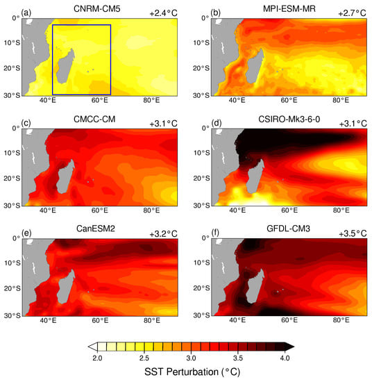
Figure 1.
CMIP5 sea-surface temperature (SST) perturbations for (a) CNRM-CM5, (b) MPI-ESM-MR (c) CMCC-CM, (d) CSIRO-Mk3-6-0, (e) CanESM2, and (f) GFDL-CM3. Perturbations are calculated by first taking the future minus present differences in the 2071–2099 and 1976–2005 means of the model data. The plotted domain corresponds to that of the ECMWF analyses with the value in the top right of each panel denoting the domain average. The blue box in (a) corresponds to the Meso-NH and CROCO simulation domains.
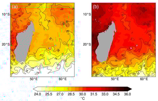
Figure 2.
Initialization SST for the present simulation (a) and multi-model-averaged future simulations (b).
Furthermore, the effect of temperature and specific humidity perturbations is shown by averaging Meso-NH air temperature and water vapor mixing ratio fields in a 500 km domain around the cyclone’s initial position (Figure 3). All CMIP5 models show low variability in the domain-averaged surface warming, with a multi-model average of +3.4 °C (+13%), as well as a slight cooling above 100 hPa. More variability exists in vertical profiles of water vapor mixing ratio with perturbations at 500 hPa varying between 0.69–1.39 g kg (+36–73%), promoting intensification with more water content aloft [37,38]. Over the entire atmospheric column, the increase in total water vapor mixing ratios range from 80 g kg to 126 g kg, corresponding to a 20–32% increase. In each of these cases, the minimum and maximum of these ranges correspond to the CNRM-CM5 and GFDL-CM3 CMIP5 models, the models with the smallest and largest impact on the historical environment.
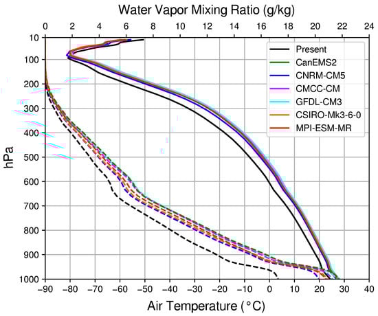
Figure 3.
Vertical profiles of air temperature (solid lines) and water vapor mixing ratio (dashed lines) averaged over a 500 km area from the initialisation position. Black solid and dashed lines represent the present climate profile while colored solid and dashed lines represent the various CMIP5 future climates, colored by model.
Once perturbations are calculated, future initial and boundary conditions are constructed by regridding air temperature, specific humidity, and surface temperature perturbations onto the ECMWF analyses domain and adding to the analysis GRIB files. These GRIB files are then pre-processed by Meso-NH, which interpolates the data onto the atmospheric grid. Similarly, perturbations for SST, ocean potential temperature, and ocean salinity are re-gridded and added to the Mercator reanalyses and pre-processed for input into CROCO.
3. Results
3.1. Trajectory
Trajectories of all simulated cyclones are determined from tracking the minimum mean sea-level pressure (MSLP) from 3-hourly Meso-NH output. However, as some cyclones exit the model domain before the end of the simulation, the last 6-h of all trajectories are truncated. These trajectories, as well as the IBTrACS best-track of Bejisa from RMSC Réunion is shown in Figure 4. In comparison to the best-track, the historical simulated cyclone reproduces the initial southward trajectory and southeastward curving towards La Réunion, albeit with a slight delay. Although Bejisa did not make landfall, its centre passed within 55 km of the western coast while that of the simulated present-climate cyclone comes within 82 km at its nearest point. The subsequent southwestward recurving after passing the island is also well reproduced with better agreement in terms of timing. Hence, except for a small westward shift due to the initial position in the ECMWF analysis being slightly southwest of the IBTrACS initial position, Bejisa’s trajectory is well reproduced in the historical simulation. Future cyclones broadly follow the same trajectory, although with an increasing westerly shift relative to the best-track and historical simulation. Such small present–future changes in the trajectory are expected, as wind perturbations were not applied to the analyses in order to maintain tracks that would impact La Réunion. Only in the CSIRO-Mk3-6-0 future simulation, in which the cyclone stalls northwestward of La Réunion before tracking southwestward, is there a substantial difference and limited passage near the island. For this reason, the CSIRO-Mk3-6-0 scenario is excluded from further analysis.
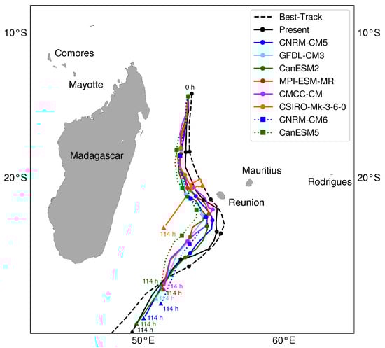
Figure 4.
Tracks of the historical best-track Cyclone Bejisa (IBTrACS; dashed black), the present-climate simulation (solid black line), and CMIP5-based future simulations (solid colors). Colored dots mark 24 h intervals and colored triangles marks 144 h, the last time at which all cyclones are still within the domain.
3.2. Intensity
In this study, all simulations started at 1200 UTC on 31 December 2013, shortly after a period of rapid intensification in which the historical Cyclone Bejisa intensified by 47 hPa in the preceding 24 h [1]. Although this period of rapid intensification is not well represented in the ECMWF analyses and is not able to be re-simulated here, all cyclones undergo an initial 12-h period of intensification followed by gradual weakening after 24–48 h (Figure 4). For each metric, the future ensemble-mean intensity is almost always greater: we find an average MSLP difference of −2 hPa and a maximum difference of −8.6 hPa at 96 h in the CanESM2 downscaling compared to present. Surface wind speeds also increases by 2 m s on average, corresponding to a 6.5% average increase, with a maximum increase of 9.39% compared to present in the CanESM2 downscaling (Table 3), which had the second highest SST perturbation. These intensity increases are consistent with the modified thermodynamic environments that are more conducive to TC intensification with higher SSTs and increased water vapor aloft. The capacity of the future environments to produce stronger cyclones is also reflected in the Maximum Potential Intensity (MPI). The MPI is a metric which estimates the theoretical maximum intensity a tropical cyclone can attain given the SST, sea level pressure, and vertical profiles of temperature, pressure, and water vapor mixing ratio. Calculating this metric ahead of each cyclone at 53 E, −20 S according to Bister and Emanuel (1998) [39], we find that all future environments support greater intensification (Table 2), highlighting the effect of the thermodynamic perturbations.
Table 2.
Summary of Maximum Potential Intensity (MPI), Lifetime Maximum Intensity (LMI), and the latitude at which LMI is attained for each simulation scenario. MPI estimates are based on the method of Bister 1998 and are calculated from Meso-NH output 3 h into each simulation at −20 S, 53 E, ahead of each cyclone. All intensities are in hPa.
In addition to these intensity changes, we find evidence of a poleward shift in the latitude of lifetime-maximum intensity (LMI) in future environments. Although when calculating LMI from maximum surface wind, an equatorward shift is detected from −22.3 S to an average of −19.8 S, in terms of MSLP, a 2.1° poleward shift is found, from −16.3 S to an average of −18.4 S (Table 2). Such a poleward shift in LMI has previously been observed in the recent best-track record and is attributed to an expansion of the tropics [40]. We find support for this argument here, with a poleward expansion of the 26 °C isotherm in time–mean composites of SST, from −25 S in the present-day environment to an average of –28.6 S in future environments (Figure 2).
In terms of previous intensity projections for this ocean basin, we find some agreement. Yamada et al. (2017) [13] cite a statistically significant −5.2 hPa strengthening, in addition to Knutson et al. (2020) [6] who report an approximate +6% increase in the median intensity, given a 2 °C global mean anthropogenic warming (see their Figure 5). Similarly, Cattiaux et al. (2020) [14] report an increase in the lifetime maximum intensity of southwest Indian ocean cyclones simulated in the CMIP6 CNRM-CM6 model, albeit with a smaller 1° poleward shift. In the only other known pseudo global warming study for a south west Indian ocean cyclone, Patricola and Wehner (2018) [41] found a statistically significant 16.8 m s increase in 10-m winds in simulating Cyclone Gafilo (2004) for a RCP8.5 scenario. Overall, intensity changes found here are qualitatively in line with established upward trends, but on the lower end of estimates for this basin.
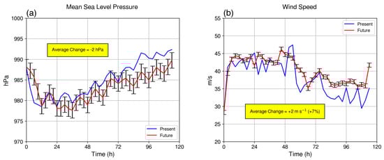
Figure 5.
Mean sea level pressure (a) and surface wind speed (b) of the present climate simulation and future climate simulations. Wind speed is calculated from the lowest model level of horizontal winds in Meso-NH (40 m). Error bars denote the standard deviation of the differences between the five future intensities and the present intensity.
3.3. Rainfall
Due to the small size of La Réunion in the basin, tropical cyclones rarely make landfall, yet the island can still be impacted by passing cyclones due to far reaching spiral rainbands [42]. Combined with the island’s volcanic interior and the associated orographic enhancement, rainfall presents a substantial threat to La Réunion and accounts for most TC-related damages and fatalities [7]. Indeed, the island holds the world record for 12 h and 24 h rainfall accumulations (1.1 m and 1.8 m respectively) from Cyclone Denise (1966) [43] and the 72 h and 96 h records (3.9 m and 4.9 m respectively) from Cyclone Gamede (2007) [44]. Hence, changes in TC-related rainfall are expected to have a considerable effect on La Réunion.
We find that rainfall rates in future cyclones are greater in all CMIP5 future scenarios (Figure 6a). On average, the median rainfall rate increases by 33.8% and by as much as 50% in the CanESM2 downscaling, again, the case with the greatest SST perturbation and despite having the weakest water vapor perturbation. Similarly, for intense rainfall, as measured by the 90th percentile rate, rainfall intensity increases by 28.6% on average, which also has a higher degree of certainty with a standard deviation of only 3% (Table 3). Qualitatively speaking, this result is inline with well-established projections for increased precipitation under climate change, both from numerous real-case modeling studies [10,11,45,46] and also on physical principles [47,48]. In the quantitative sense, increases found here are on the higher end of projections for the south Indian ocean under an aggregated 2 K mean global warming [6]. However, in terms of RCP8.5 based scenarios, our estimates are comparatively smaller (see Table ES4, Supplementary Information, [6]), such as +41.6% in the case of a future Cyclone Gafilo [41], also simulated with non-paramaterized convection as used here. Additionally, we calculate a 28.4% average increase in rainfall rates averaged within 100 km of the cyclone center (Figure 6b), exceeding past estimates for this basin [49]. Although any increase may be tied to the relative SST warming (i.e., basin warming vs tropical average warming), the average SST perturbation applied here nearly match that of the tropical average warming calculated from our CMIP5 ensemble (+3 K vs. +2.9 K). One possible explanation for our higher projections therefore is the use of a 3 km resolution, allowing an explicit representation of deep convection, which cannot be resolved explicitly in current global models.
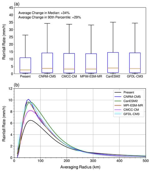
Figure 6.
All rainfall rates (mm/h) within 100 km of the cyclone center for each simulation (a) and composite rainfall rates with radius from the cyclone center for each simulation (b). In (a), red horizontal lines represent sample medians and the lower and upper extents of blue rectangles represent the 75th and 25th quartiles, respectively. The upper and lower whiskers represent the effective maximum and minimum values of the data after filtering for outliers. Outliers are determined as data points that are greater than Q3 + 1.5 IQR and less than Q1 − 1.5 IQR, where Q1 is the 25th percentile, Q3 is the 75th percentile, and IQR is the interquartile range.
Table 3.
The percentage change in all examined cyclone characteristics for each CMIP5 downscaling with respect to the present control simulation. Multi-model averages are given on the bottom row with the sample standard deviations in parentheses.
Furthermore, our estimates of changes in rainfall over La Réunion itself will be conservative, as orographic enhancement effects have not been taken into account. Projections calculated here are based on rainfall rates for ocean grid points, given our limited ability to represent the island’s orography with a 3-km grid spacing. Additionally, rainfall over the island depends strongly on cyclone size, intensity, and the distance of the cyclone from the coast (i.e., trajectory), making it difficult to attribute changes in island rainfall rates to different future environments. Indeed, a grid spacing of less than 1 km may be necessary to accurately simulate the intensity and spatial variability of orographic precipitation over La Réunion [42]. Although orographic rainfall studies for future climates indicate an increase in precipitation with height [50], an increase in intensity [51], or a shift in the precipitating area towards the leeward side [52], high-resolution microscale modelling is necessary to estimate future changes unique to La Réunion. One possible avenue for future research is to use the output from these simulations to downscale to higher-resolution simulations over the island.
3.4. TC Size
Just as passing cyclones can still affect La Réunion due to their spiral rainbands, so too can gale-force outer winds cause damage. TC size in terms of wind structure is therefore another important characteristic to consider. Cyclone size in this study is calculated from the radius of 17.5 m s (34-kt) and 33 m s (64-kt) winds, signifying the thresholds for a ‘Moderate Tropical Storm’ and a ‘Tropical Cyclone’ respectively in the South West Indian Ocean. These thresholds can also be interpreted as representing the outer-storm environment for winds of 17.5 m s and the inner-storm environment for winds of 33 m s. For the inner-storm environment, although we find an average 2.3% increase in the radius of 33 m s winds, the standard deviation is , with a range from −6–10% (Table 3), suggesting this result is not significant (Figure 7). However, we find consensus for a contraction of the outer-storm environment, with a 9.2% average decrease in the 17.5 m s wind radius, from an average of 292 km in the historical simulation to 266 km in future simulations. This decrease is also seen in terms of precipitation, with averaged rainfall rates slightly smaller beyond 300 km (Figure 6b). Additionally, radar reflectivities were averaged in 5-km bands around a cyclone’s center for each point on its trajectory to construct Hovmöller composites, which also highlight a shrinking precipitating area. Whereas in the historical simulation, this area extends to 450 km, in future cyclones, it grows initially during the first 72 h and is thereafter largely confined to 330 km on average (Figure 8).
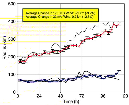
Figure 7.
Average radius of the 17.5 m s wind and 33 m s wind. For the present control simulation, the black solid line represents the 33 m s wind radius and black dotted line represents the 17.5 m s wind radius. For future climate simulations, the blue (red) line represent the multi-model mean 33 m s (17.5 m s) wind radius. Error bars are as described in Figure 5, but for the 17.5 m s and 33 m s wind radii.
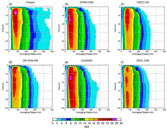
Figure 8.
Hovmöller of radar reflectivity at 1.5 km above sea level (ASL) averaged by radius from cyclone center for each simulation. (a) Present; (b) CNRM-CM5; (c) CMCC-CM; (d) MPI-ESM-MR; (e) CanESM2; (f) GFDL-CM3.
The physical mechanisms behind this decrease are potentially related to reduced air–sea fluxes and the modulation of convection in the outer-storm environment. In the context of global warming, the argument is laid out by Sun et al. (2017) [53]: SST warming in the outer-storm environment leads to an increase in the surface entropy flux that enhances convective instability in the lower troposphere. In turn, rainband formation and diabatic heating is promoted, further enhancing low-level convergence, the acceleration of tangential winds, and hence a larger storm. However, whereas Sun et al. (2017) [53] only considers SST warming, air temperature and specific humidity perturbations are also applied in this study. Although a moister outer environment has been shown to promote TC size [54], the temperature and humidity perturbations applied here result in a moistening of the lower troposphere and a slightly greater near-surface warming compared to SST warming by 0.2 K on average. Surface moisture and entropy fluxes are thus reduced in the outer-storm environment, reducing convective instability, deep convection, and any associated increase in surface winds.
Whether the reduction found here contributes to an emerging trend however is uncertain. Our results find some agreement with those of Parker et al. (2018) [10] who find a decrease in the 17.5 m s wind radius in re-simulating Cyclone Ita (2014) in northeastern Australia under a RCP8.5 scenario. Similarly, Lynn et al. (2009) [55] find a decrease in storm size for a Hurricane Katrina-like cyclone at the end of the 21st century, albeit for a radius of “strong winds”. For the south Indian ocean in particular, Kim et al. (2014) [56] find a statistically significant increase in the radius of 25 m s winds under a CO doubling scenario, but no change in the radius of 12 m s winds. On the other hand, Knutson et al. (2015) [49] and Yamada et al. (2017) [13] find an increase in the 12 m s wind radius under a CO doubling scenario. Evidently there remains much uncertainty on TC size projections, not just for the south Indian ocean, but globally. Although any change in TC size is expected to be less than 10%, there is no consensus between basins, nor even on the sign on this change [6]. Further modeling of TC size under cloud-resolving resolutions is therefore necessary to build consensus.
3.5. Significant Wave Height
In addition to the characteristic changes discussed so far, increases in sea level, coupled with greater coastal development, is expected to compound oceanic impacts from tropical cyclones [5,6,15,57,58]. In this study, changes in the TC-ocean characteristics are examined in terms of the significant wave height. The significant wave height is defined as the average of the highest one-third of waves and is outputted every 1 h from WAVEWATCH III simulations performed in-post, with initial and boundary conditions provided by 1 hourly surface wind output from Meso-NH. Tracking the maximum wave height for each output time reveals that future wave heights closely resemble those in the present control. Across future downscalings, we find changes of 0.76, 1.11, −0.08, 0.14, and −0.15 m, with an average of 0.36 m which translate to +4.61% ±4.76% in term of percentage change (Figure 9). Thus, as the variation rivals the average change, no clear projection of wave height is evident.
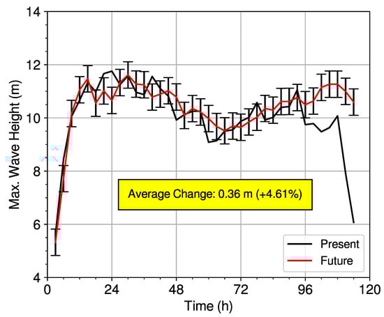
Figure 9.
Maximum of the significant wave height (m) for the historical simulation (black) and the future mean of maximum wave heights from CMIP5 downscaled simulations (red). Error bars are as described in Figure 5, but for maximum wave height.
Furthermore, one must also bear in mind that surface wind speed is only one factor modulating wave height. One other substantial factor that will contribute to future wave height is sea level change. To assess this contribution, we calculated sea surface height changes according to the RCP8.5 scenario in the same way as for the other perturbations used in this study. We find that the DJFMA averaged fields show a large degree of inter-model variability, not only in the spatial pattern of sea level change, but in its sign (Figure 10). On the scale of the South Indian Ocean, most models (four out of six) exhibit a dipole rise and fall in sea level, rising over the northwest of the basin (exceeding 15 cm north east of Madagascar) and sinking levels over the southeast of the basin. The increases seen over the northwest of the basin are possibly indicative of a trend towards more frequent strong Indian Ocean Dipole events in the future [59]. In the southeast of the basin, the falls in sea level are confined to zonally-oriented channels that extend as far west as La Réunion and Mauritius. In this region, five out of the six CMIP5 models project sea level will fall by 0–10 cm. As future wave height changes found here are mostly positive and can be up to 1 m, the significant wave height may contribute as much, or even more, to cyclonic swell than sea level change, compared to present. These competing contributions require further investigation, not only around La Réunion, but in other parts of the basin, such as off the northeastern coast of Africa, where prominent ocean warming and sea level rise would support substantial wave risk.
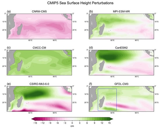
Figure 10.
CMIP5 sea surface height perturbations for (a) CNRM-CM5, (b) MPI-ESM-MR (c) CMCC-CM, (d) CanESM2, (e) CSIRO-Mk3-6-0, and (f) GFDL-CM3. Perturbations are calculated by first taking the future minus present differences in the 2071–2099 and 1976–2005 means of the model data. The plotted domain corresponds to that of the ECMWF analyses with the Meso-NH and CROCO simulation domains shown in blue in (f).
4. Summary and Conclusions
High-resolution, ocean–atmosphere coupled simulations have been used to project future characteristic changes in a Bejisa-like cyclone for the South West Indian Ocean. An ensemble of simulations has been conducted, consisting of a re-simulation of the historical cyclone that passed nearby La Réunion in early 2014 and six simulations of Bejisa-like cyclones within potential future environments of the late 21st century. Future environments have been constructed using the pseudo global warming method, in which perturbations to operational analyses of the historical synoptic environment are calculated from six CMIP5 climate models according to the IPCC’s RCP8.5 emissions scenario.
Although this method has been used extensively in the literature for future tropical cyclone projections, one must bear in mind some caveats about its implicit assumptions. For example, we start our simulations at a time when a mature cyclone has already developed, presuming the potential for future cyclogenesis in this region. However, Cattiaux et al. (2020) [14] indicate a mixed future signal in the potential for cyclogenesis in this region (see their Figure 5c and Figure 8e), giving us confidence that our assumption is at least not unfounded. Additionally, multi-year averaged perturbations have been used that suppress peaks and troughs in teleconnection signals, such as the Indian Ocean Dipole which modulates SST patterns across the basin. One would expect future periods of higher SST and humidity relative to the present to have a greater effect on storm intensity, precipitation, and possibly size. This study has also focused on only one cyclone and its associated large-scale environment and an investigation for multiple cyclones would offer a larger sample size and more precise projections. Finally, these projections are based on a climatologically moderate cyclone and further work examining changes associated with a stronger cyclone, such as Cyclone Idai (2019), would be beneficial to explore. Indeed, the modelling methodology presented in this article does not intend to furnish exhaustive projections, but to complement other larger scale studies presented in this special issue and elsewhere that investigate future cyclonic risk in the South Indian Ocean [14,60].
However, in terms of the specific case of Cyclone Bejisa, we find that the historical track is well reproduced, although with a slight westward shift. The evolution of the historical intensity is well reproduced, with a period of short intensification followed by a gradual decay. On the other hand, the magnitude of historical intensity was underestimated in our model, possibly because simulations start at a time when the historical Cyclone Bejisa was exiting a phase of rapid intensification that was underestimated in the ECMWF analyses used. However, as the aim of this study is to consider present–future changes in TC characteristics, the lack of an exact recreation of the historical intensity, although desirable, is not considered detrimental to the following main findings of this study.
In future environments, we find that the cyclone trajectory remains largely unchanged albeit with a slight westward shift, an expected result as we do not perturb the historical wind pattern. Furthermore, we find that future cyclones are 6.5% more intense on average due to imposed SST and humidity perturbations and that the lifetime maximum intensity is attained further poleward by an average of 2 degrees, in agreement with a future expansion of the tropics. Additionally, imposed CMIP5 perturbations also result in a 33.8% increase in the median rainfall rate and as a 28.6% increase in intense rainfall rates, as measured by the 90th percentile. Future cyclones are also smaller, with a 9.2% decrease in the radius of outer 17.5 m s winds. Calculating wind-induced significant wave height from Meso-NH surface winds further reveals an approximate 4.6% increase in the significant wave height. Although wave height projections were highly variable, most were positive and could offset the decrease in sea surface height projected by CMIP5 around La Réunion. Thus, we find that future Bejisa-like cyclones would be more intense, smaller, produce heavier rainfall, and mostly generate larger ocean waves. Coupled with expected increases in population and coastal development, such cyclones pose an increased threat to La Réunion and the wider basin, which is already home to some of the world’s poorest countries.
Author Contributions
Conceptualization, C.B., S.B. and P.T.; methodology, C.T., C.B. and S.B.; validation, C.T.; C.T.; investigation, C.T.; data curation, C.T.; writing–original draft preparation, C.T.; writing–review and editing, C.T., C.B., S.B., P.T. and J.P.; visualization, C.T.; supervision, C.B., S.B., P.T. and J.P.; project administration, C.B., S.B., P.T.; funding acquisition, C.B. All authors have read and agreed to the published version of the manuscript.
Funding
This study was funded by the European Union, La Réunion Regional Council and the French state under the framework of the INTERREG-5 Indian Ocean 2014–2020 project “ReNovRisk Cyclones and Climate Change".
Acknowledgments
We give thanks to Meteo-France in Toulouse, France on whose Beaufix supercomputer these simulations were performed. The numerical models used are freely available at the following websites: http://mesonh.aero.obs-mip.fr/mesonh51forMeso-NH (access on 5 February 2021), https://www.croco-ocean.org/ (access on 5 February 2021) for CROCO, and https://github.com/NOAA-EMC/WW3/ (access on 5 February 2021) for WW3. We thank the World Climate Research Programme’s Working Group on Coupled Modelling, which is responsible for CMIP, and we thank the climate modeling groups (listed in Table 1 of this paper) for producing and making their model output freely available via the Earth System Grid Federation (ESGF) web portals (https://esgf-node.llnl.gov/projects/cmip5/ (access on 5 February 2021)). Finally, we thank three anonymous reviewers for their feedback and comments which has improved the quality of this work.
Conflicts of Interest
The authors declare no conflict of interest.
Appendix A

Figure A1.
Mean sea level pressure (a) and surface wind speed (b) and rainfall rates within 100 km (c) for the historical simulation, the CNRM-CM5- and CanESM2-based future simulations (solid colored lines in (a,b)), and the CNRM-CM6- and CanESM5-based future simulations (dashed colored lines in (a,b)).

References
- Pianezze, J.; Barthe, C.; Bielli, S.; Tulet, P.; Jullien, S.; Cambon, G.; Bousquet, O.; Claeys, M.; Cordier, E. A New Coupled Ocean-Waves-Atmosphere Model Designed for Tropical Storm Studies: Example of Tropical Cyclone Bejisa (2013–2014) in the South-West Indian Ocean. J. Adv. Model. Earth Syst. 2018, 10, 801–825. [Google Scholar] [CrossRef]
- Kuleshov, Y.; Fawcett, R.; Qi, L.; Trewin, B.; Jones, D.; McBride, J.; Ramsay, H. Trends in tropical cyclones in the South Indian Ocean and the South Pacific Ocean. J. Geophys. Res. 2010, 115, D01101. [Google Scholar] [CrossRef]
- Holland, G.; Bruyère, C.L. Recent intense hurricane response to global climate change. Clim. Dyn. 2014, 42, 617–627. [Google Scholar] [CrossRef]
- Kossin, J.P.; Knapp, K.R.; Olander, T.L.; Velden, C.S. Global increase in major tropical cyclone exceedance probability over the past four decades. Proc. Natl. Acad. Sci. USA 2020. [Google Scholar] [CrossRef]
- Walsh, K.J.; McBride, J.L.; Klotzbach, P.J.; Balachandran, S.; Camargo, S.J.; Holland, G.; Knutson, T.; Kossin, J.P.; Lee, T.C.; Sobel, A.; et al. Tropical cyclones and climate change. Wiley Interdiscip. Rev. Clim. Change 2016, 7, 65–89. [Google Scholar] [CrossRef]
- Knutson, T.; Camargo, S.J.; Chan, J.C.L.; Emanuel, K.; Ho, C.H.; Kossin, J.; Mohapatra, M.; Satoh, M.; Sugi, M.; Walsh, K.; et al. Tropical Cyclones and Climate Change Assessment: Part II: Projected Response to Anthropogenic Warming. Bull. Am. Meteorol. Soc. 2020, 101, E303–E322. [Google Scholar] [CrossRef]
- Needham, H.F.; Keim, B.D.; Sathiaraj, D. A review of tropical cyclone-generated storm surges: Global data sources, observations, and impacts. Rev. Geophys. 2015, 53, 545–591. [Google Scholar] [CrossRef]
- Schär, C.; Frei, C.; Lüthi, D.; Davies, H.C. Surrogate climate-change scenarios for regional climate models. Geophys. Res. Lett. 1996, 23, 669–672. [Google Scholar] [CrossRef]
- Lackmann, G.M. Hurricane Sandy before 1900 and after 2100. Bull. Am. Meteorol. Soc. 2015, 96, 547–560. [Google Scholar] [CrossRef]
- Parker, C.L.; Bruyère, C.L.; Mooney, P.A.; Lynch, A.H. The response of land-falling tropical cyclone characteristics to projected climate change in northeast Australia. Clim. Dyn. 2018, 51, 3467–3485. [Google Scholar] [CrossRef]
- Mittal, R.; Tewari, M.; Radhakrishnan, C.; Ray, P.; Singh, T.; Nickerson, A.K. Response of tropical cyclone Phailin (2013) in the Bay of Bengal to climate perturbations. Clim. Dyn. 2019, 53, 2013–2030. [Google Scholar] [CrossRef]
- Emanuel, K.A. Downscaling CMIP5 climate models shows increased tropical cyclone activity over the 21st century. Proc. Natl. Acad. Sci. USA 2013, 110, 12219–12224. [Google Scholar] [CrossRef]
- Yamada, Y.; Satoh, M.; Sugi, M.; Kodama, C.; Noda, A.T.; Nakano, M.; Nasuno, T. Response of Tropical Cyclone Activity and Structure to Global Warming in a High-Resolution Global Nonhydrostatic Model. J. Clim. 2017, 30, 9703–9724. [Google Scholar] [CrossRef]
- Cattiaux, J.; Chauvin, F.; Bousquet, O.; Malardel, S.; Tsai, C.L. Projected changes in the southern Indian ocean cyclone activity assessed from high-resolution experiments and CMIP5 models. J. Clim. 2020. [Google Scholar] [CrossRef]
- Knutson, T.; McBride, J.L.; Chan, J.; Emanuel, K.; Holland, G.; Landsea, C.; Held, I.; Kossin, J.P.; Srivastava, A.K.; Sugi, M. Tropical cyclones and climate change. Nat. Geosci. 2010, 3, 157–163. [Google Scholar] [CrossRef]
- Global Guide. Global Guide to Tropical Cyclone Forecasting; World Meteorological Organization: Geneva, Switzerland, 2017; p. 397. [Google Scholar]
- Jumeaux, G.; Quetelard, H.; Roy, D. Atlas Climatique de La Réunion; La Documentation Française: Paris, France, 2011. [Google Scholar]
- Leroux, M.D.; Meister, J.; Mekies, D.; Dorla, A.L.; Caroff, P. A Climatology of Southwest Indian Ocean Tropical Systems: Their Number, Tracks, Impacts, Sizes, Empirical Maximum Potential Intensity, and Intensity Changes. J. Appl. Meteorol. Climatol. 2018, 57, 1021–1041. [Google Scholar] [CrossRef]
- Lac, C.; Chaboureau, J.P.; Masson, V.; Pinty, J.P.; Tulet, P.; Escobar, J.; Leriche, M.; Barthe, C.; Aouizerats, B.; Augros, C.; et al. Overview of the Meso-NH model version 5.4 and its applications. Geosci. Model Dev. 2018, 11, 1929–1969. [Google Scholar] [CrossRef]
- Caniaux, G.; Redelsperger, J.L.; Lafore, J.P. A Numerical Study of the Stratiform Region of a Fast-Moving Squall Line. Part I: General Description and Water and Heat Budgets. J. Atmos. Sci. 1994, 51, 2046–2074. [Google Scholar] [CrossRef]
- Pinty, J.P.; Jabouille, P. A mixed-phased cloud parameterization for use in a mesoscale non-hydrostatic model: Simulations of a squall line and of orographic precipitation. In Proceedings of the Conference on Cloud Physics, Everett, WA, USA, 17–21 August 1998. [Google Scholar]
- Lunet, T.; Lac, C.; Auguste, F.; Visentin, F.; Masson, V.; Escobar, J. Combination of WENO and Explicit Runge–Kutta Methods for Wind Transport in the Meso-NH Model. Mon. Weather Rev. 2017, 145, 3817–3838. [Google Scholar] [CrossRef]
- Bechtold, P.; Bazile, E.; Guichard, F.; Mascart, P.; Richard, E. A mass-flux convection scheme for regional and global models. Q. J. R. Meteorol. Soc. 2001, 127, 869–886. [Google Scholar] [CrossRef]
- Cuxart, J.; Bougeault, P.; Redelsperger, J.L. A turbulence scheme allowing for mesoscale and large-eddy simulations. Q. J. R. Meteorol. Soc. 2000, 126, 1–30. [Google Scholar] [CrossRef]
- Mlawer, E.J.; Taubman, S.J.; Brown, P.D.; Iacono, M.J.; Clough, S.A. Radiative transfer for inhomogeneous atmospheres: RRTM, a validated correlated-k model for the longwave. J. Geophys. Res. 1997, 102, 16663–16682. [Google Scholar] [CrossRef]
- Fouquart, Y.; Bonnel, B. Computations of Solar Heating of the Earth’s Atmosphere—A New Parameterization. Beitr. Phys. Atmos. 1980, 53, 35–62. [Google Scholar]
- Tolman, H.L. Effects of Numerics on the Physics in a Third-Generation Wind-Wave Model. J. Phys. Oceanogr. 1992, 22, 1095–1111. [Google Scholar] [CrossRef]
- Sherwood, S.C.; Ingram, W.; Tsushima, Y.; Satoh, M.; Roberts, M.; Vidale, P.L.; O’Gorman, P.A. Relative humidity changes in a warmer climate. J. Geophys. Res. Atmos. 2010, 115. [Google Scholar] [CrossRef]
- Taylor, K.E.; Stouffer, R.J.; Meehl, G.A. An Overview of CMIP5 and the experiment design. Bull. Am. Meteorol. Soc. 2012, 93, 485–498. [Google Scholar] [CrossRef]
- IPCC. Climate Change 2013: The Physical Science Basis. Contribution of Working Group I to the Fifth Assessment Report of the Intergovernmental Panel on Climate Change; Cambridge University Press: Cambridge, UK, 2013; p. 1535. [Google Scholar] [CrossRef]
- Donner, L.J.; Wyman, B.L.; Hemler, R.S.; Horowitz, L.W.; Ming, Y.; Zhao, M.; Golaz, J.C.; Ginoux, P.; Lin, S.J.; Schwarzkopf, M.D.; et al. The Dynamical Core, Physical Parameterizations, and Basic Simulation Characteristics of the Atmospheric Component AM3 of the GFDL Global Coupled Model CM3. J. Clim. 2011, 24, 3484–3519. [Google Scholar] [CrossRef]
- Giorgetta, M.A.; Jungclaus, J.; Reick, C.H.; Legutke, S.; Bader, J.; Böttinger, M.; Brovkin, V.; Crueger, T.; Esch, M.; Fieg, K.; et al. Climate and carbon cycle changes from 1850 to 2100 in MPI-ESM simulations for the Coupled Model Intercomparison Project phase 5. J. Adv. Model. Earth Syst. 2013, 5, 572–597. [Google Scholar] [CrossRef]
- Voldoire, A.; Sanchez-Gomez, E.; Salas y Melia, D.; Decharme, B.; Cassou, C.; Senesi, S.; Valcke, S.; Beau, I.; Alias, A.; Chevallier, M.; et al. The CNRM-CM5.1 global climate model: Description and basic evaluation. Clim. Dyn. 2013, 40, 2091–2121. [Google Scholar] [CrossRef]
- Yu, B.; Li, G.; Chen, S.; Lin, H. The role of internal variability in climate change projections of North American surface air temperature and temperature extremes in CanESM2 large ensemble simulations. Clim. Dyn. 2020, 55. [Google Scholar] [CrossRef]
- Collier, M.; Rotstayn, L.; Kim, K.Y.; Hirst, A.; Jeffrey, S. Ocean circulation response to anthropogenic-aerosol and greenhouse gas forcing in the CSIRO-Mk3.6 coupled climate model. Aust. Meteorol. Oceanogr. J. 2013, 63, 27–39. [Google Scholar] [CrossRef]
- Scoccimarro, E.; Gualdi, S.; Bellucci, A.; Sanna, A.; Fogli, P.G.; Manzini, E.; Vichi, M.; Oddo, P.; Navarra, A. Effects of Tropical Cyclones on Ocean Heat Transport in a High-Resolution Coupled General Circulation Model. J. Clim. 2011, 24, 4368–4384. [Google Scholar] [CrossRef]
- Gray, W.M. Global View of the Origin of Tropical Disturbances and Storms. Mon. Weather Rev. 1968, 96, 669–700. [Google Scholar] [CrossRef]
- Montgomery, M.T. Introduction to Hurricane Dynamics: Tropical Cyclone Intensification. In Advanced Numerical Modeling and Data Assimilation Techniques for Tropical Cyclone Predictions; Mohanty, U.C., Gopalakrishnan, S., Eds.; Springer: Berlin/Heidelberg, Germany, 2016; pp. 537–559. [Google Scholar] [CrossRef]
- Bister, M.; Emanuel, K.A. Dissipative heating and hurricane intensity. Meteorol. Atmos. Phys. 1998, 65, 1436–5065. [Google Scholar] [CrossRef]
- Kossin, J.P.; Emanuel, K.A.; Vecchi, G.A. The poleward migration of the location of tropical cyclone maximum intensity. Nature 2014, 1476–4687. [Google Scholar] [CrossRef] [PubMed]
- Patricola, C.M.; Wehner, M.F. Anthropogenic influences on major tropical cyclone events. Nature 2018, 563, 1476–4687. [Google Scholar] [CrossRef] [PubMed]
- Pohl, B.; Morel, B.; Barthe, C.; Bousquet, O. Regionalizing Rainfall at Very High Resolution over La Réunion Island: A Case Study for Tropical Cyclone Ando. Mon. Weather Rev. 2016, 144, 4081–4099. [Google Scholar] [CrossRef]
- Holland, G. WMO/TC-No. 560, Report No. TCP-31, World Meteorological Organization. 1993. Available online: https://wmo.asu.edu/content/world-greatest-twenty-four-hour-1-day-rainfall (accessed on 5 February 2021).
- Quetelard, H.; Bessemoulin, P.; Peterson, T.C.; Burton, A.; Boodhoo, Y.; Cerveny, R.S. WMO CCl Rapporteur for climate extremes decision, World Meteorological Organization. 2007. Available online: https://wmo.asu.edu/content/world-greatest-ninety-six-hour-4-day-rainfall (accessed on 5 February 2021).
- Wang, C.C.; Lin, B.X.; Chen, C.T.; Lo, S.H. Quantifying the Effects of Long-Term Climate Change on Tropical Cyclone Rainfall Using a Cloud-Resolving Model: Examples of Two Landfall Typhoons in Taiwan. J. Clim. 2015, 28, 66–85. [Google Scholar] [CrossRef]
- Gutmann, E.D.; Rasmussen, R.M.; Liu, C.; Ikeda, K.; Bruyere, C.L.; Done, J.M.; Garrè, L.; Friis-Hansen, P.; Veldore, V. Changes in Hurricanes from a 13-Yr Convection-Permitting Pseudo—Global Warming Simulation. J. Clim. 2018, 31, 3643–3657. [Google Scholar] [CrossRef]
- Allen, M.R.; Ingram, W.J. Constraints on future changes in climate and the hydrologic cycle. Nature 2002, 419, 1476–4687. [Google Scholar] [CrossRef]
- Pall, P.; Allen, M.R. Testing the Clausius–Clapeyron constraint on changes in extreme precipitation under CO2 warming. Clim. Dyn. 2007, 28, 351–363. [Google Scholar] [CrossRef]
- Knutson, T.; Sirutis, J.J.; Zhao, M.; Tuleya, R.E.; Bender, M.; Vecchi, G.A.; Villarini, G.; Chavas, D. Global Projections of Intense Tropical Cyclone Activity for the Late Twenty-First Century from Dynamical Downscaling of CMIP5/RCP4.5 Scenarios. J. Clim. 2015, 28, 7203–7224. [Google Scholar] [CrossRef]
- Napoli, A.; Crespi, A.; Ragone, F.; Maugeri, M.; Pasquero, C. Variability of orographic enhancement of precipitation in the Alpine regione. Sci. Rep. 2014, 9, 2045–2322. [Google Scholar] [CrossRef]
- Shi, X.; Durran, D.R. Estimating the Response of Extreme Precipitation over Midlatitude Mountains to Global Warming. J. Clim. 2015, 28, 4246–4262. [Google Scholar] [CrossRef]
- Siler, N.; Roe, G. How will orographic precipitation respond to surface warming? An idealized thermodynamic perspective. Geophys. Res. Lett. 2014, 41, 2606–2613. [Google Scholar] [CrossRef]
- Sun, Y.; Zhong, Z.; Li, T.; Yi, L.; Hu, Y.; Wan, H.; Chen, H.; Liao, Q.; Ma, C.; Li, Q. Impact of Ocean Warming on Tropical Cyclone Size and Its Destructiveness. Sci. Rep. 2017, 7, 8154. [Google Scholar] [CrossRef] [PubMed]
- Hill, K.A.; Lackmann, G.M. Influence of Environmental Humidity on Tropical Cyclone Size. Mon. Weather Rev. 2009, 137, 3294–3315. [Google Scholar] [CrossRef]
- Lynn, B.H.; Healy, R.; Druyan, L.M. Investigation of Hurricane Katrina characteristics for future, warmer climates. Clim. Res. 2009, 39, 75–86. [Google Scholar] [CrossRef]
- Kim, H.S.; Vecchi, G.A.; Knutson, T.; Anderson, W.G.; Delworth, T.L.; Rosati, A.; Zeng, F.; Zhao, M. Tropical Cyclone Simulation and Response to CO2 Doubling in the GFDL CM2.5 High-Resolution Coupled Climate Model. J. Clim. 2014, 27, 8034–8054. [Google Scholar] [CrossRef]
- Lin, N.; Emanuel, K.; Oppenheimer, M.; Vanmarcke, E. Physically based assessment of hurricane surge threat under climate change. Nat. Clim. Chang. 2012, 2, 462–467. [Google Scholar] [CrossRef]
- Chen, J.; Wang, Z.; Tam, C.Y.; Lau, N.C.; Lau, D.S.D.; Mok, H.Y. Impacts of climate change on tropical cyclones and induced storm surges in the Pearl River Delta region using pseudo-global-warming method. Sci. Rep. 2020, 10, 1965. [Google Scholar] [CrossRef]
- Cai, W.; Yang, K.; Wu, L.; Huang, G.; Santoso, A.; Ng, B.; Wang, G.; Yamagata, T. Opposite response of strong and moderate positive Indian Ocean Dipole to global warming. Nat. Clim. Chang. 2021, 11, 27–32. [Google Scholar] [CrossRef]
- Tsai, C.L.; Bousquet, O.; Malardel, S.; Cattiaux, J.; Chauvin, F. Impact of Globe Warming on Tropical Depression Characteristics in Southwest Indian Ocean Investigating by High-resolution ARPGEG Simulations. Atmosphere 2020. submitted. [Google Scholar]


Publisher’s Note: MDPI stays neutral with regard to jurisdictional claims in published maps and institutional affiliations. |
© 2021 by the authors. Licensee MDPI, Basel, Switzerland. This article is an open access article distributed under the terms and conditions of the Creative Commons Attribution (CC BY) license (http://creativecommons.org/licenses/by/4.0/).