Application of a Common Methodology to Select in Situ CO₂ Observations Representative of the Atmospheric Background to an Italian Collaborative Network

Abstract

We describe and implement a data selection algorithm aimed at identifying background atmospheric CO₂ observations from in situ continuous measurements. Several selection criteria for detecting the background data have been developed and are currently used: the main objective of this work was to define a common methodology to extract the atmospheric background signal minimizing heterogeneities due to the use of different selection algorithms. The algorithm used in this study, (BaDS, Background Data Selection) was tested and optimized using data (from 2014 to 2018) from four Italian stations characterized by markedly different environmental conditions (i.e., mountain, coastal and marine): Plateau Rosa (PRS), Mt. Cimone (CMN), Capo Granitola (CGR) and Lampedusa (LMP). Their locations extend from the Alps to the central Mediterranean. The adopted algorithm proved to be effective in separating the local/regional from the background signal in the CO₂ time series. About 6% of the data at LMP, 11% at PRS, 20–38% at CMN and 65% at CGR were identified as non-background. LMP and PRS can be used as reference sites for the central Mediterranean, while CMN and CGR were more impacted by regional sources and sinks. Finally, we discuss a possible application of BaDS screened data.

1. Introduction

The Mediterranean basin is considered a global hot-spot region for climate change and air-quality. CO₂ is the single most-important anthropogenic greenhouse gas (GHG) in the atmosphere, accounting approximatively for 62% of the anthropogenic radiative forcing by long-lived GHGs. Fossil fuel and cement production emissions are the main drivers for the increasing atmospheric CO₂ dry mole fraction in the global atmosphere [1].

In response to this, regulation and emission trading schemes have been adopted at international, national, and city levels to reduce GHG emissions, while responding to the needs for economic and societal development. The successful implementation of GHG emission reductions must be guided by reliable scientific evidence. While satellite observations and ground-based remote sensing measurements have gained importance in recent decades [2,3,4], global and regional networks of in situ GHG observations still largely represent the reference information for GHG monitoring, emission and variability studies [1,5,6]. These networks are characterized by significant efforts dedicated to the harmonization and increased comparability of GHG observations [7,8,9].

The analysis and interpretation of atmospheric mole fraction time series play a fundamental role in assessing long-term trends and interannual growth rates of CO₂. To this aim, it is pivotal to extract the information related to the atmospheric background from the data series, i.e., data “representative of the global atmosphere not affected by local conditions” [10]. The identification of the background signal in the GHG time series is also necessary to isolate data, which yields information related to processes occurring at regional scales, i.e., regional fluxes [11]. Usually, remote islands or high-mountain sites are indicated as suitable locations to trace the background atmospheric levels of atmospheric species. However, as shown in previous studies [12,13,14,15,16,17,18,19], even at island or high-mountain sites, the influence of direct anthropogenic and natural emissions cannot be neglected.

For these reasons, selection criteria have been developed and used to identify measurements directly affected by emission or removal processes, and to retain data that are well representative of the atmospheric background [10,20,21]. For CO₂, some of these approaches are based on the following common strategy to identify non-background data: a polynomial equation is used to remove the long-term CO₂ trend, then a harmonic function is applied to reproduce the seasonal variation, and (finally) residual variations are determined. To separate the seasonal component from long-term trend and irregular variations (i.e., time series decomposition), different approaches can be used: “HPspline” [22,23,24], CCGCRV (Carbon Cycle Group CuRVe) [25,26,27], Seasonal Trend decomposition (STL) [28] or least square fitting methods [29]. However, to infer information related to latitudinal gradients, regional fluxes, and large-scale temporal variability, it is necessary to apply these decomposition techniques to a subset of data that are representative of the atmospheric background. Different methodologies exist to extract the background data from the time series of atmospheric constituents: the robust extraction of a baseline signal (REBS and 2-D-REBS) [30,31], the adaptive selection of diurnal minimum variation (ADVS) [21], the coefficient of variation (COV) [32] and the standard deviation of the background (SD) [33]. A comparison study between COV, SD and REBS approaches applied to four stations with different environmental conditions contributing to the Integrated Carbon Observation System, ICOS (http://www.icos-cp.eu, accessed on 9 December 2020), European Union research infrastructure, was carried out by El Yazidi et al. [34]. According to their results, the SD and REBS methodologies are the most flexible for spike detection across different sites, but REBS tends to underestimate spikes when these are very high. Instead, the SD methodology appears to better detect data not belonging to the baseline. Giostra et al. [20] proposed the use of a statistical filter that identifies the data baseline, i.e., the subset of data in a time series which are not significantly affected by non-well-mixed contributions. By assuming that a well-mixed species follows a Gaussian distribution, the observed CO₂ molar fraction probability density function (PDF) should be fitted with the sum of a Gaussian PDF and a Gamma PDF (the latter describing the non-well-mixed data). All the data for which the corresponding Gaussian is higher than the Gamma PDF are assigned to the baseline. Among the different approaches, the method of Thoning et al. [25], initially developed for the measurements of Mauna Loa Station, has been widely used. It consists of two steps which analyze the variability of the hourly CO₂ data (i.e., their standard deviation) and the difference between consecutive hourly means. Then, an iterative algorithm removes any values which differ from the weighted spline curve by more than a given threshold. Due to its simple usability and the lack of any strong pre-requisite regarding the measurement site environmental conditions, it has been applied to other remote stations, for example, Schauninsland, a site in the southwest of Germany [35], Junfgraujoch (Switzerland), Puy de Dôme (France) [36], and four WMO/GAW (Global Atmosphere Watch programme of the World Meteorological Organization) stations in China [37].

In this study, we tested the application of the background data selection algorithm presented by Apadula et al. [19], called BaDS (Background Data Selection) to five different datasets of in situ continuous CO₂ observations in Italy, belonging to a collaborative network. This algorithm is based on the method of Thoning et al. [25], and has some common points with the methodology already used by Cundari et al. [38]. With respect to [19], we paid particular attention to applying a robust identification of the threshold value used to discriminate the CO₂ variability (i.e., impacted by large-scale vs. regional/local phenomena). The aim of this study is to evaluate the ability of the BaDS methodology in extracting the information related to the background variability from CO₂ time series recorded at fixed monitoring stations with substantially different characteristics: mountain, coastal and marine sites. This will permit verifying if, by using a common approach, we can obtain a consistent view of the background CO₂ variability at the different sites of the observational network. Moreover, the identification of measurement periods representative of the atmospheric background also has the co-advantage of permitting identification of the periods which are above or below the atmospheric background, thus allowing for the specific characterization of the measurement sites. This latter point is particularly important when assessing the capability of a measurement site in catching signals useful for the quantification and spatial allocation of anthropogenic or natural emissions/sinks.

Even if most of these observatories have longer datasets [19,29,39], only a subset of 5 years has been used to test the methodology. Indeed, a long-term analysis is beyond the scope of this paper. Section 2 reports a description of the measurement sites, of the experimental setup, and of the background data selection algorithm (BaDS). The daily and the seasonal variability of the different CO₂ datasets, with an analysis of the impact of the data selection algorithm are discussed in Section 3. In Section 3, we also provide an example of the BaDS application for the investigation of the interannual variability of the seasonal cycles. A discussion on the method, with implications and future research directions, is provided in Section 4. Conclusions are drawn in Section 5.

2. Experiments

2.1. Measurement Sites

This study considered near-surface CO₂ measurements from four laboratories (CAMM, ENEA, National Research Council of Italy—Institute for Atmospheric Sciences and Climate (CNR—ISAC) and RSE S.p.A.) at the four atmospheric observatories, the location of which is shown in Figure 1. The geographical locations of these observatories (spanning from north to south across the Italian peninsula, separated by more than 1200 km and more than 10° latitude, and from sea level up to 3480 m a.s.l.) provides the opportunity to investigate the spatial and temporal variability of greenhouse gases over Italy and the central Mediterranean basin. In the classification of Henne et al. [15], Lampedusa (LMP) was classified as a generally remote site and Mt. Cimone (CMN) as weakly influenced by regional emissions. Plateau Rosa (PRS) can be considered similar to the near site of Jungfraujoch (JFJ, at 3571 m a.s.l. on the Switzerland Alps), classified by Henne et al. [15] as a mostly remote site.

The main aim of this work was to test and implement a methodology for background data selection to verify its performance and usefulness for obtaining a coherent baseline dataset. We considered only a limited period of observations (see

Table 1. Measurement period considered in this study for each site/laboratory.

PRS	CMN—ISAC	CMN—CAMM	CGR	LMP
2014–2018	2018	2015–2018	2015–2018	2014–2018

) starting from 2014 to the end of 2018, with measurements based on a similar experimental setup, i.e., using cavity ring-down spectroscopy (CRDS) analyzers. Measurements based on the CRDS technique were started at LMP in 2012, at Capo Granitola (CGR) in 2015, while two instruments operated at CMN: the Italian Air Force (CAMM) provided CRDS data from 2015, while the National Research Council of Italy—Institute for Atmospheric Sciences and Climate (CNR—ISAC) started CRDS measurements in 2018.

The PRS station is part of the Testa Grigia Observatory (45°56′ N 7°42′ E, 3480 m a.s.l., http://oasi.rse-web.it/, accessed on 9 December 2020), a high mountainous site in the Italian western Alps far from potential pollutant sources. It is situated over an Alpine glacier, often above the planetary boundary layer (PBL), devoid of soil and vegetation. These characteristics make the station suitable for background measurements of greenhouse gases. Incursion events of polluted air masses from the European plains rarely occur at the PRS site [17]. More information on the measurement site can be found in [19]. PRS contributes to WMO/GAW as a regional station. This site is under the labelling processes to join the ICOS Research Infrastructure. The dataset used in this work is available at the World Data Center for Greenhouse Gases (WDCGG) by the WMO/GAW (see https://gaw.kishou.go.jp/, accessed on 9 December 2020).

CMN (44°12′ N, 10°42′ E, 2165 m a.s.l.) is the highest peak of the northern Apennines. This mountain range separates the European continent from the Mediterranean regions. The site is characterized by a free horizon for 360° and is far from big cities and important industrial areas (Bologna and Florence are located more than 50 km away and are 2 km below the station). CMN is considered to be well representative of the free tropospheric condition, even if direct transport of air masses from the regional PBL can be systematically observed, especially during the warm months [13,40]. In particular, as observed by Colombo et al. [13], during May–September, the CO₂ variability is significantly affected by the diurnal vertical transport of air masses, which produces a decrease in the atmospheric molar ratio due to photosynthetic uptake by vegetation. The atmospheric observatory, composed by the Italian Air Force meteorological station (located at the mountain top) and the “O. Vittori” CNR observatory (located about 50 m below the mountain top, see http://cimone.isac.cnr.it/, accessed on 9 December 2020), is a WMO/GAW global station [41]. The “O. Vittori” observatory was approved as an ICOS atmospheric class 2 site in November 2018. The dataset considered for the CAMM laboratory was extracted by WDCGG. The dataset for the CNR laboratory was extracted from the ICOS dataset for the period May–December 2018 (Cristofanelli et al., 2020 “ICOS CO₂ release”, see https://data.icos-cp.eu/, accessed on 9 December 2020) [42], while for the period January–April 2018 an “interim” dataset (for which the ICOS protocols were not fully implemented) was considered.

The CGR station (37°34′ N, 12°40′ E, 15 m a.s.l.; http://www.i-amica.it/i-amica/?page_id=632 accessed on 9 December 2020) is managed by CNR and is located on the south-western coast of Sicily, overlooking the Sicily channel, in the central Mediterranean. The observatory has been operational since 2014 and contributes to WMO/GAW as a regional station. Thanks to its semi-background location, various studies about the atmospheric processes influencing the variability of traces gases and aerosol [43,44] and the characterization of the Mediterranean Sea background conditions have been carried out [45]. This measurement site is strongly affected by the land/sea breeze regime, which leads to the advection of background air masses from offshore during the daytime, and polluted air masses from inner Sicily during the nighttime [43]. This observatory is located within the CNR scientific campus at Torretta Granitola (a small village 12 km from Mazara del Vallo, 12,000 inhabitants). The shelter where the observatory is hosted is situated on a cliff (15 m high) overlooking the coastline. The dataset used for this analysis is available at the WCDGG by WMO/GAW.

The ENEA Atmospheric Observatory LMP (35°31′ N, 12°38′ E, 45 m a.s.l.; http://www.lampedusa.enea.it/ accessed on 9 December 2020) is located on the island of Lampedusa. Lampedusa is a small island (about 22 km² surface area, 6000 inhabitants) more than 100 km from the African continent, and more than 200 km South of Sicily. The island is flat, with sparse vegetation, and limited local emission sources. In the study by Henne et al. (2010) [15], the site was characterized as the most remote (together with Mace Head, in Ireland), out of 34 different European considered sites. The atmospheric observatory is located on a 45 m plateau, on the north-eastern coast of the island. Several parallel measurement programs aimed at the long-term monitoring of climate and investigating climate-related processes are carried out at the observatory [46]. Previous studies [47] have shown that the Lampedusa CO₂ record is characterized by a very limited diurnal cycle; this is due to the very limited impact of local sources and sinks, and the reduced daily variability of the planetary boundary layer in the open sea. Since 1992, this observatory has been contributing as a WMO/GAW regional station. LMP also contributes to the US National Oceanic and Atmospheric Administration Global Greenhouse Gas Reference network (https://www.esrl.noaa.gov/gmd/ccgg/ggrn.php accessed on 9 December 2020). On May 2020, the LMP station was labelled as a “class-2” atmospheric station within ICOS. The dataset considered for LMP was produced by ENEA and is available at the WCDGG by WMO/GAW.

2.2. Background Data Selection Algorithm (BaDS)

We tested and adopted a methodology (BaDS—Background Data Selection) originally applied at PRS [19] and based on the classical data selection used at the Mauna Loa observatory [48]. BaDS is based on the assumption that background observations are characterized by a low temporal variability because they should not be affected by nearby emissions or removal processes. In this work, BaDS was applied to time series of mean hourly CO₂ values. Before BaDs application, short data gaps due to calibrations or outages were filled using a simple linear interpolation. The procedure, summarized below, consisted of 3 steps.

Firstly, hourly mean values were selected as a function of their respective standard deviation, calculated from the 1 min mean values: only data with hourly standard deviation <1 ppm were retained. The selected data were then used to: (a) calculate a running median on 504 h (21 days), and (b) calculate the average difference between consecutive hourly mean values (defined as the “S” parameter).

Secondly, the differences (ΔC) between the retained hourly values and the corresponding 504-h running median values were calculated. A confidence interval equal to n * S, where n was a variable parameter defined by the user, was calculated. All data points with |ΔC|> n * S were discarded. Basically, through this step all the outliers were rejected from the dataset.

Thirdly, 48 h running means were calculated using the data retained by the previous step. The differences (δC) between hourly mean values (with σ < 1 ppm) and the corresponding 48 h running means were then calculated. All data points with |δC|> n * S were flagged as “non background”.

It should be noted, that during Step 1 (i.e., calculation of the reference running median and “S” parameter), only nighttime observations (i.e., under mountain breeze regime, considered less affected by local/regional contributions) were considered from May to September for the CMN—ISAC and CMN—CAMM datasets. Similarly, only observations during daytime (i.e., under sea breeze regime) were considered for CGR. In this way, the impact of vegetation uptake under the thermal upward wind regime (at CMN) and the impact of anthropogenic emissions transported under land breeze circulation (at CGR) have been minimized. The complete datasets were considered in the analysis for PRS and LMP.

A critical aspect for this method was the determination of the value of n. In [19], the value of n is determined based on expert judgement and good knowledge of the site data. Since data from different sites are considered in this study, we have developed an improved (and less arbitrary) method for the determination of n.

A sensitivity study was carried out to define, for each dataset, the optimal values of the parameter n. The procedure was applied for n ranging from 1 to 15. Two separate tests have been performed on each dataset. The first test aimed to assess the influence of the parameter n on the number of non-background data, in order to verify the method selection capability and to avoid creating under representative datasets. The second test was performed to evaluate the effect of the parameter n to the diurnal CO₂ cycle amplitude under background conditions. As denoted by the analysis of the original dataset, each measurement site was characterized by a typical diurnal variation cycle whose amplitude is a function of the proximity of source/sink regions (

Table 2. Median amplitude of the diurnal variation (expressed in ppm) and percent of data removed (in brackets) for each measurement site. The values of S and of the retrieved optimal n parameters are reported for each site.

Dataset	PRS n = 6 S = 0.36	CMN—ISAC n = 5 S = 0.52	CMN—CAMM n = 6 S = 0.36	CGR n = 1 S = 1.43	LMP n = 10 S = 0.30
Original	0.78	4.47	3.80	8.90	0.58
Background	0.33 (11%)	1.59 (38%)	0.75 (20%)	1.60 (65%)	0.64 (6%)

). The lowest median amplitude characterized the diurnal cycle at PRS and LMP (0.78 and 0.58 ppm, respectively). Despite its elevation, CMN is affected by a mountain breeze regime which favors the advection of air masses from the PBL during the daytime of warm months (May–September), resulting in a larger median amplitude of the CO₂ diurnal cycle (3.80 ppm for CMN—CAMM and 4.47 ppm for CMN—ISAC). The largest median amplitude of the diurnal cycle was found at CGR (8.9 ppm), due to the influence of the marine breeze regime which advects (relatively clean) marine air masses during the daytime and (polluted) air masses from inland during the nighttime. Since the CO₂ diurnal variability is expected to be minimized at the measurement sites for background conditions, the second test was performed to identify the optimal n values which reduce this amplitude. We believe this provided a useful criterion for the determination of the optimal n value to be used to detect the background data. To this aim, for each station, the median amplitude of the diurnal cycle (calculated over the whole dataset for each site/laboratory) was calculated as a function of the background dataset obtained by applying different n values. The results of both sensitivity tests are shown in Figure 2.

In general, for CMN—ISAC and CMN—CAMM, the minima in the median diel CO₂ cycle amplitude were found at n = 5 and n = 6, respectively. For LMP and PRS, only a limited dependency was found on the n value, while the strongest dependency was found for CGR with the lowest median CO₂ cycle amplitude at n = 1. Thus, setting n = 6 and n = 10 for PRS and LMP represented a good compromise to minimize the (already low) diel CO₂ cycle amplitudes and to retain a usable fraction of data as representative of background.

Results for CGR showed a different behavior with respect to the other datasets, with a somewhat larger daily cycle amplitude, and a fraction of rejected data which denoted only a limited dependency on the n value. Interestingly, differences were evident between CMN—CAMM and CMN—ISAC as concerning the dependence of the diel CO₂ cycle amplitude and the fraction of data retained as “background” as a function of the adopted n values. This is related to the different temporal data coverages of these dataset. Indeed, the optimal value of n = 5 was obtained for both CMN—CAMM and CMN—ISAC when only data for one year (2018) were considered.

As is apparent from Table 2, it is evident that the application of BaDS was effective in reducing the diurnal cycle, by decreasing the impact of local/regional emissions or removal processes at all the measurement sites. In particular, the amplitude of the diurnal cycle was strongly reduced at CMN (for both ISAC and CAMM dataset a 4-fold reduction was obtained) and CGR (8-fold reduction). At these sites a significant fraction of the data (considering the whole datasets) was rejected by BaDS as non-background: 38 and 20% at CMN—ISAC and CMN—CAMM, 65% at CGR. The impact of BaDS on the median diurnal cycles at PRS and LMP was less evident (even if still discernible at PRS) due to the lower impact of local/regional emission/removal processes at these sites, as also testified by the low fraction of removed record (11% for PRS and 8% for LMP). Based on these results, LMP can be considered as being well representative of the baseline conditions of the central Mediterranean basin, and its comparison with the dataset from other sites can provide hints to discuss the CO₂ variability over Italy.

The optimal overall threshold used in the selection, equal to n * S, is very similar for PRS, LMP, and CMN (between 2.16 and 2.6 ppm). A much smaller threshold was needed at CGR to isolate the background conditions from the totality of observations.

A further sensitivity test was performed with the aim of assessing the impact to the BaDS results of applying, for each measurement site, different n values calculated on a seasonal basis.

Table 3. Median amplitude of the diurnal variation (expressed in ppm) and percentage of data removed (in brackets) for each measurement site using seasonal values of n. The values of S and of the retrieved optimal n parameters are reported for each site.

Dataset	PRS n winter = 4 n spring = 8 n summer = 6 n autumn = 5 S = 0.36	CMN-ISAC n winter = 4 n spring = 10 n summer = 2 n autumn = 10 S = 0.52	CMN-CAMM n winter = 5 n spring = 14 n summer = 6 n autumn = 7 S = 0.36	CGR n winter = 1 n spring = 1 n summer = 2 n autumn = 2 S = 1.43	LMP n winter = 8 n spring = 8 n summer = 5 n autumn = 14 S = 0.30
Original	0.78	4.47	3.80	8.90	0.58
Background	0.33 (15%)	2.00 (31%)	0.79 (21%)	1.80 (56%)	0.81 (10%)

reports, for each measurement site, the fraction of data discarded and not representative of the atmospheric background when the seasonally-derived n values were used in BaDS. In respect to the annually-derived n values (Table 2), the use of the seasonally calculated n values led to differences in the fraction of discarded data (Table 3 and

Table 4. For each analyzed dataset, percentage of data discarded by adopting in BaDS the annually-derived or the seasonally-derived n values.

Dataset	CMN—ISAC	CMN—CAMM	LMP	CGR	PRS
Annually-derived n	38.2%	20.3%	6.1%	65.3%	10.7%
Seasonally-derived n	31.2%	21.4%	9.9%	55.6%	14.5%

) that ranged from −9.7% at CGR to +3.8% at PRS. The agreement between the two approaches was 90% (LMP), 83% (PRS), 74% (CMN—CAMM), 55% (CMN—ISAC), and 30% (CGR), defined as the percentage of data that was retained as background simultaneously by using the annual and the seasonal n value. For all the measurement sites (but not for PRS), the median amplitude of the CO₂ diel cycle was minimized when adopting the annual n value. Only for PRS was there no difference between the two approaches: this was probably due to its remote location, more consistently representative of the atmospheric background and less affected by local source/sink through the seasons of the year. Thus, based on these results, we decided to use the n value obtained on the annual basis in the BaDS.

3. Results

3.1. Analysis of CO₂ Diurnal Variation and Impact of BaDS Application

With the purpose of assessing the impact of the BaDS selection on the typical CO₂ diurnal cycle at each measurement site, we calculated the seasonal (winter: DJF, spring: MAM, summer: JJA, autumn: SON) average diurnal variations of the detrended CO₂ hourly values for the original dataset and for the background selection (after the BaDS application). For each dataset, the detrended values have been obtained by subtracting from the hourly values the corresponding value of the fit obtained applying the Equation (1) from [29]:

$$\mathrm{y}={\mathrm{c}}_1+{\mathrm{c}}_2\mathrm{m}+\mathrm{A}\sin \left[\frac{2\mathsf{\pi }\left(\mathrm{m}+{\mathsf{\phi }}_1\right)}{{\mathrm{T}}_1}\right]+\mathrm{B}\sin \left[\frac{2\mathsf{\pi }\left(\mathrm{m}+{\mathsf{\phi }}_2\right)}{{\mathrm{T}}_2}\right]$$

(1)

where y is the monthly CO₂ molar fraction, c₁ and c₂ are constant values, m is the incremental number of months, T₁ and T₂ represent semi-annual and annual periods (6 months and 12 months, respectively), φ₁ and φ₂ are the semi-annual and annual phases, respectively. The parameters obtained from the fit are shown in

Table 5. Parameter of the fit (Equation (1)) to the background-selected dataset (monthly mean).

Fitting Parameters	PRS	CMN—CAMM	CGR	LMP
A	1.42	0.96	1.11	−1.16
B	5.11	6.00	4.92	4.40
c1 (ppm)	397.17	400.00	401.29	397.60
c2 (ppm month−1)	0.216	0.225	0.182	0.214
φ1 (months)	−14.50	−1.72	−0.11	−0.02
φ2 (months)	1.37	1.98	3.83	1.10
r2	0.94	0.96	0.90	0.86
n. points	59	47	44	58

. Results for the calculated seasonal average diurnal cycles are shown in Figure 3.

For the original datasets (Figure 3, top), a small diurnal cycle amplitude (less than 1 ppm) characterized PRS and LMP during all seasons. A significant diurnal cycle (with lower values during daytime) was evident for CMN in summer (average amplitude: 5.5 ppm) for both the ISAC and CAMM datasets, in good agreement with the summer variability observed by Ref. [13]. The diurnal cycle at CMN, as previously discussed, was attributed to the systematic thermal transport of PBL air masses up to the mountain peak during daytime; the valley breeze brings air masses that are depleted in CO₂ to the measurement site due to the vegetation sink, favored by the presence of woods on the slopes of the mountain [13]. The summer PRS diurnal cycle was about 2.5 ppm, in agreement with Schmidt et al. [35], who suggested that the amplitude of the summer diurnal cycle in mountain sites is inversely proportional to the altitude. Small differences appeared between CMN—ISAC and CMN—CAMM, which were primarily related to the different data coverage (only one full year for CMN—ISAC), even if an impact from the different sampling heights [50] cannot be completely neglected. The largest diurnal cycle amplitudes were observed for CGR, with seasonal amplitudes ranging from 8 ppm in winter to 12 ppm in summer. As discussed above, this was linked to the influence of the marine breeze regime and the influence of regional sources and sinks. Fires from agricultural residues and uncontrolled landfills that occurred within the territory might have provided additional anthropogenic CO₂ sources that contributed to produce a marked daily cycle. As also reported by Cristofanelli et al. [43] and, for other coastal sites in Sicily, by Perrino et al. [51], during all the seasons CGR showed strongly higher pollutants concentrations than LMP during nighttime (due to the advection of air masses from inner Sicily, affected by anthropogenic sources and by the effect of soil and vegetation as a sources of respiratory CO₂) and more comparable values during daytime (due to the advection of marine air masses representative of the Mediterranean basin PBL).

The diurnal cycles at CGR were significantly reduced in amplitude for the background data selected by BaDS (Figure 3, bottom). This was true also for the summer data at PRS and CMN. For CGR, the shape and average values of the background diurnal cycle approached those observed at LMP. Even if the difference from LMP was strongly reduced, at CGR, signals of regional anthropogenic emissions were probably still reflected by the higher values (especially during summer nighttime). Especially during spring, the CGR background average diurnal cycle approached that observed at LMP, stressing the ability of BaDS in selecting measurement periods representative of the atmospheric background even at a measurement site strongly exposed to anthropogenic emissions.

For the background datasets, lower CO₂ values were typically observed at PRS (−1.5 ppm, on average) with respect to LMP. During winter the tropospheric CO₂ is characterized by a vertical gradient with the highest CO₂ levels near the surface due to biogenic and anthropogenic emissions [52], and it is reasonable to suggest that PRS is more affected by free tropospheric air masses compared to LMP. During the vegetative season, it is likely that the lower CO₂ values observed at PRS and CMN were tracing a background latitudinal gradient between continental and oceanic regions in the Mediterranean basin. With respect to LMP, slightly higher values (+0.5 ppm) were instead observed for CMN—CAMM during the central part of the day in winter, possibly indicating a residual role of upward thermal transport of air masses from the PBL. The opposite situation was observed in summer daytime, when the mountain sites (especially CMN) were more exposed to the transport of air masses from the PBL (Figure 3 bottom).

3.2. Analysis of CO₂ Time Series and Impact of BaDS Application

Figure 4 shows the CO₂ monthly mean time series at the different sites from 2014 to 2018 by considering the original datasets, and the monthly time series of the background CO₂ dataset, as obtained by the BaDS application. Apart from the multi-year increasing tendency, the seasonal variations of CO₂ through the years is evident, with maxima in the first months of each year, a minima during summer, and an amplitude of the annual cycle of about 10–15 ppm, depending on the year and the measurement site. The seasonal CO₂ cycle was a combination of different contributions: biosphere emission and removal processes, anthropogenic emissions and atmospheric transport (on different temporal and spatial scales).

The different time series selected with BaDS were more consistent with each other than the original datasets. Only the CMN—ISAC dataset was still characterized by the appearance of the high CO₂ values during February 2018, significantly higher than those observed for CMN—CAMM. Additionally, the application of BaDS based on the seasonal-derived n parameter (Section 2.2) does not allow for the detection and removal of high CO₂ values in February 2018, which were related to the occurrence of specific multi-day peak events observed at CMN—ISAC (please note that these events were not present in the CMN—CAMM dataset due to a stricter flagging strategy adopted at this laboratory: i.e., data points that consistently deviated from the rest of the dataset were rejected by a data screening process performed by station operators on the raw data). This would suggest that BaDS (at least with the parameter configuration indicated in Section 2.2) was not able to correctly identify the multi-day pollution episodes occurring in this month as non-background data. The methodology performed well during the winter season and also during pollution events; however, elevated CO₂ cases lasting for numerous days remain problematic with this algorithm.

3.3. Analysis of CO₂ Seasonal Cycle and Impact of BaDS Application

To better characterize the impact of the BaDS application on the determination of the CO₂ seasonal cycle at the different sites, we calculated the average monthly mean values of the detrended CO₂ (Figure 5, left) over the whole periods of data availability by using the same methodology used for the analysis of the diurnal cycle (see Section 3.1). This has been done for the original dataset and for background dataset. In the original dataset, we observed similar seasonal cycles for PRS and LMP: both sites showed an annual minimum in August and a maximum in March. CMN (both ISAC and CAMM dataset) was denoted by a different shape of the average annual cycle with a more marked (and fast) decrease in May–July with respect to PRS and LMP, reflecting a more marked signature of the continental photosynthetic activity. This led to the occurrence of a broader summer minimum at CMN than at PRS and LMP. Marked differences existed between the CO₂ average values during the cold months (February–March and November–December) between ISAC and CAMM dataset at CMN. As already explained in Section 3.2 this was related to the different flagging strategies adopted at the two laboratories. The CO₂ seasonal cycle was significantly larger at CGR than at the other sites. As discussed above, especially during nighttime (under the land-breeze regime), CGR was also more directly affected by anthropogenic CO₂ emissions due to fires from agricultural residues and uncontrolled burning of landfills that occurred within the regional territory. Although characterized by more vegetation than LMP, the monthly difference at CGR with respect to LMP did not decrease in summer. This may be due to the hot summer that characterizes these territories, favoring a more dry and arid soil, affecting the vegetation and thereby reducing CO₂ uptake. In addition to this lack of vegetative uptake, an increase in CO₂ emissions due to touristic activity cannot be neglected, as suggested by the seasonal increase observed for other anthropogenic co-emitted compounds (e.g., NOx, CO, SO₂) [43].

The differences among the different seasonal cycles were minimized after BaDS application (Figure 5, right). If we exclude the CMN—ISAC dataset, for which high values were still observed in January and February (even if notably reduced in respect to the original dataset), the differences between the different measurement sites are reduced to 2.5 ppm (from October to March) and to less than 1 ppm (July). In particular, the decreasing phase of the annual cycle from April to August was similar for all sites, with the CMN dataset approaching PRS and LMP. The outstanding agreement of the CGR background to the other sites demonstrates the ability of the BaDS algorithm to extract the background signal even if the measurement site was strongly impacted by local/regional emissions.

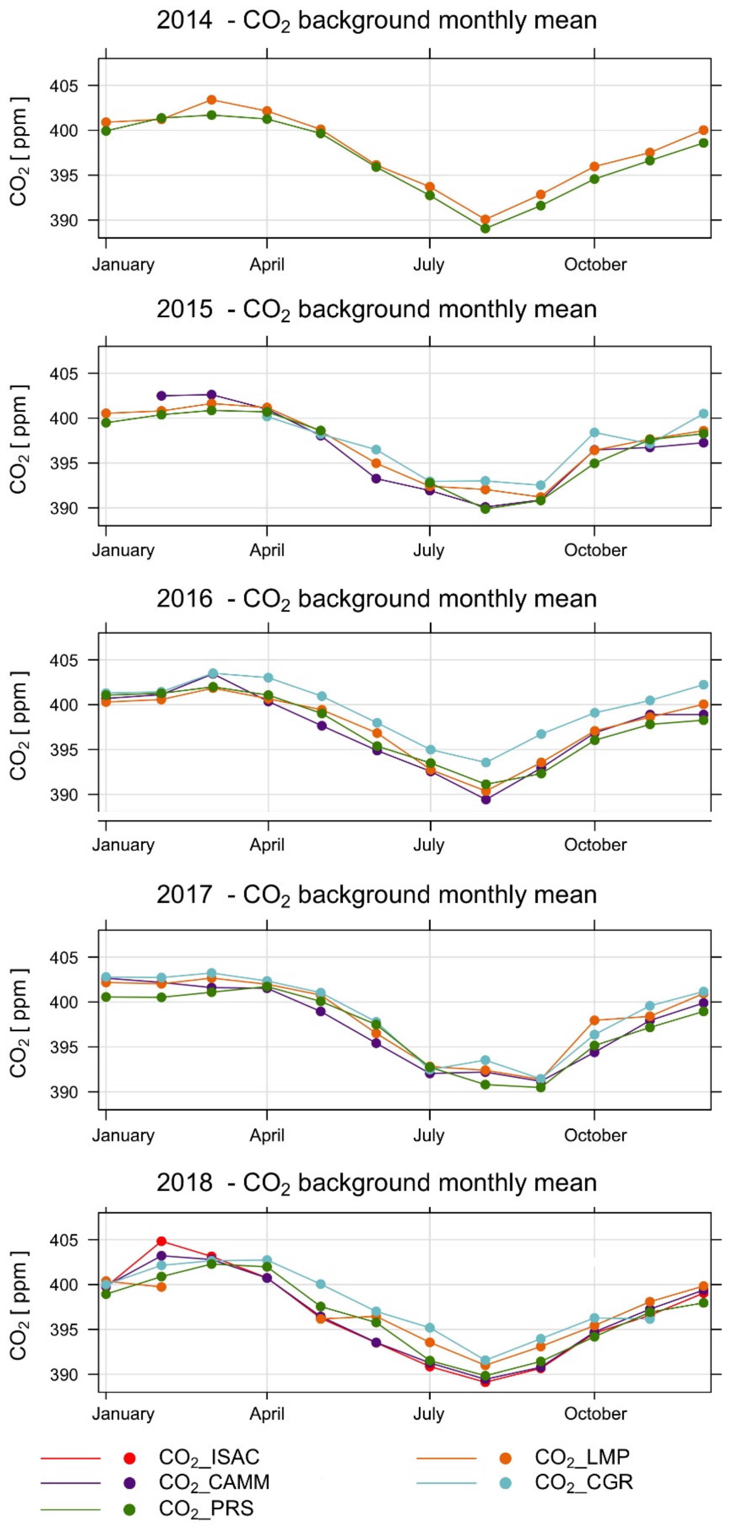
3.4. Use Case of the BaDS Application: Investigation of Interannual Variability of the Seasonal CO₂ Cycle

With the purpose of providing an example of a possible application of the BaDS algorithm, we analyzed the interannual variability of the seasonal cycles of background CO₂ data at the four observatories belonging to the Italian collaborative network. In order to quantify annual and semi-annual components, Equation (1) from [29] was fit to the CO₂ monthly mean values for the background data selection with BaDS (Table 5).

The largest annual cycle amplitude (calculated as |2xB|) was found for CMN—CAMM (12.0 ppm) and the lowest for LMP (8.8 ppm). Intermediate values were found for PRS (10.2 ppm) and CGR (9.8 ppm). This clearly confirmed the lower regional/continental influence at LMP (less affected by vegetation uptake in summer and anthropogenic emission in winter) as well as a larger exposure of CMN to regional/continental emission/removal processes. The values of the seasonal cycle amplitude showed a positive gradient with latitude, indicating a decreasing influence of continental sources/sinks moving from northern to southern sites.

Figure 6 shows the annual cycles for the different datasets and the different years. An interannual modulation of the summer minimum is evident. Consistently, all the dataset shows a broader summer minimum in 2015 and 2017, while a narrower minimum appearing in August in 2014, 2016, and 2018. This phenomenon was related to a lower decrease in CO₂ values in August during years 2015 and 2017, which might suggest less efficient uptake by vegetation during these years and/or increased CO₂ emissions, possibly linked to forest fires. Murayama et al. [53], by examining the role of atmospheric circulation variability in affecting the interannual variability of the observed atmospheric CO₂ growth rate in the Northern Hemisphere, suggested that the variability of the summer atmospheric CO₂ decrease can be the result of the synergistic action of variability in biospheric sources and air-mass transport, as deduced by analysis of the North Atlantic Oscillation (NAO) and the Pacific–North America (PNA) modes.

4. Discussion

In order to discriminate CO₂ observations as representative and non-representative of atmospheric background conditions at the four measurement sites spanning from the Alps to the central Mediterranean, we implemented the methodology presented in Ref. [19] (BaDS). BaDS is a pre-conditioning algorithm for extracting time periods representative of the atmospheric background conditions from time series of CO₂ derived by in situ continuous observations. Due to differences in the environmental characteristics of the measurement sites, a specific strategy was used to identify the most appropriate tuning of the parameters involved in the data filtering.

We showed that the implemented methodology has the capability to reduce, from the original time series, the impact of local/regional CO₂ fluxes, thus extracting a signal more related to the atmospheric CO₂ background. In particular, it also performed well at CGR, a measurement site characterized by a complex interaction of anthropogenic emissions, vegetation uptake and a sea breeze wind regime. After the BaDS application, the consistency of the monthly mean CO₂ values strongly increased among the considered measurement sites. A notable exception was the CMN—ISAC dataset which showed a divergent average value in February 2018. For this specific month, BaDS did not appear to identify a long-lasting pollution event (corroborated by the simultaneous increase in CO and NO₂) which affected the measurement site. This episode was characterized by an overall increase in CO₂ for several days: it is likely that the lack of high-frequency variability prevented the attribution of this episode to the non-background conditions.

The comparison among the CMN—ISAC dataset (for which one full year of data are available) and the CMN—CAMM dataset (for which three full years of data are considered), suggested that the length of the time series can affect the BaDS output, thus creating a certain degree of uncertainty in the selection process. As shown by Table 2, the different lengths of the time series lead to different optimal “n” values and different amplitudes of the diurnal CO₂ cycle for the background dataset. When only 1 year of data were considered for CMN—CAMM, more consistent results were found with CMN—ISAC. Based on preliminary tests carried out by considering an extended CMN—ISAC time series (2018–2019, here not shown), we argue that the background data selection increases in robustness when longer time series are used.

With the aim of evaluating the impact of tuning the “n” parameter in respect to the original BaDS setting used in Ref. [19], we compared BaDS results for the PRS station using n = 7 (according with Ref. [19]) and n = 6 (according with our optimal tuning). As regards our optimal tuning, for the background selection, the original BaDS application lead to a larger amplitude of the diurnal CO₂ cycle (0.42 ppm) with a lower number of discarded data (8%). This would suggest that, in respect to the “expert” subjective setting proposed by Ref. [19], the optimal “tuning” is more effective in leaving out the residual signals that are unrelated to background conditions. However, the parameter “n” selected in this study, was obtained by applying the methodology to a shorter time series in respect to Ref. [19] and this might have led to a different optimal value for “n”.

The BaDS capability to identify the CO₂ measurement period representative of the atmospheric background in different environmental conditions (from the high mountain to a coastal site influenced by anthropogenic emissions, and to a remote marine site) may allow for further studies concerning the long-term CO₂ variability by using a larger number of measurement sites. However, as demonstrated in this work, a fine-tuning method is recommended to set the proper value of a key parameter (n) for optimizing the selection procedure: this optimal value is dependent on the measurement site and on the length of the time series. This implies that the adoption of a full common set-up for all the measurement sites still remains a challenging goal.

5. Conclusions

In this work, we assessed the capability of a data selection methodology (BaDS) for identifying the observations representative of the atmospheric background from the time series of near-surface CO₂ (hourly mean values) at four permanent observatories in Italy from 2014 to 2018: Plateau Rosa, Mt. Cimone, Capo Granitola, and Lampedusa. These observatories are located in different environmental conditions and latitudinal/altitudinal ranges, and are managed by different institutions. In addition to providing hints about the ability of BaDS in detecting background data, the systematic comparison of the CO₂ dataset recorded at these observatories is also relevant to investigate the dependence of the observed CO₂ variability as a function of altitude and latitude in Italy. In respect to the original BaDS application performed by Apadula et al. [19], we implemented a more objective definition of the key parameter n which tunes the confidence interval to retain data points as representative of the atmospheric background. After this specific tuning of the key parameter n, 94 and 89% of the data were selected as representative of the background conditions at LMP and PRS, respectively. A larger fraction of data was determined as non-background at CMN, with a maximum occurrence of non-background data at CGR (65%). A more coherent diurnal and seasonal CO₂ evolution among the various datasets was obtained after BaDS application.

Considering the original dataset (i.e., without BaDS application), a low average diurnal amplitude (less than 1 ppm) characterized PRS and LMP during all seasons, while a significant diurnal cycle was evident at CMN during vegetative growing months (mostly due to the vertical transport of air masses depleted in CO₂ due to vegetation photosynthesis) and CGR (due to the transport of air masses affected by anthropogenic emissions during nighttime). After BaDS application, the diurnal CO₂ cycle was strongly reduced at CMN and CGR. At PRS and LMP the diurnal cycle amplitude remained lower than 1 ppm. Due to the high altitude at PRS, and the very remote location at LMP, these sites were less affected by emission or removal processes at regional scales. This was also shown by the larger seasonal cycle observed at CMN (12 ppm) with respect to the other sites, and the lowest seasonal amplitude at LMP (8.8 ppm). Based on these results, the LMP and PRS dataset can be considered well representative of the baseline conditions of the central Mediterranean basin, while CMN (especially in summer) and CGR are suitable locations to systematically assess the influence of emissions and sinks occurring within the regional PBL.

Based on our results, after a correct tuning of the setting parameter “n”, the BaDS methodology appeared to be able to identify data affected by sources/sink of CO₂ and to extract the information about the background variability at the selected sites which display very different environmental characteristics. Here, we tested BaDs over a set of CO₂ datasets observed in Italy. Its usage at other measurement sites may be the object of further investigation.

Finally, as a further application of the method, we showed how we can retrieve robust information on the regional variability of the annual cycle. Despite large differences in the original datasets, a coherent evolution, with broader summer minima at all sites during 2015 and 2017, was obtained from the analysis of the background data. In this paper, the performance of BaDS methodology have been evaluated on a set of data produced by the Italian network, but it will be interesting to verify the application at different monitoring sites, such as the European infrastructure network ICOS, and evaluate the performance in respect to other methodologies present in the literature (e.g., Refs. [20,30,31,32,33]) in a future work.

References

1. Friedlingstein, P.; Jones, M.W.; O’Sullivan, M.; Andrew, R.M.; Hauck, J.; Peters, G.P.; Peters, W.; Pongratz, J.; Sitch, S.; Le Quéré, C.; et al. Global Carbon Budget 2019. Earth Syst. Sci. Data 2019, 11, 1783–1838. [Google Scholar] [CrossRef] [Green Version]
2. Bergamaschi, P.; Houweling, S.; Segers, A.; Krol, M.; Frankenberg, C.; Scheepmaker, R.A.; Dlugokencky, E.; Wofsy, S.C.; Kort, E.A.; Sweeney, C.; et al. Atmospheric CH4 in the first decade of the 21st century: Inverse modeling analysis using SCIAMACHY satellite retrievals and NOAA surface measurements. J. Geophys. Res. Atmos. 2013, 118, 7350–7369. [Google Scholar] [CrossRef] [Green Version]
3. Alexe, M.; Bergamaschi, P.; Segers, A.; Detmers, R.; Butz, A.; Hasekamp, O.; Guerlet, S.; Parker, R.; Boesch, H.; Frankenberg, C.; et al. Inverse modelling of CH4 emissions for 2010–2011 using different satellite retrieval products from GOSAT and SCIAMACHY. Atmos. Chem. Phys. 2015, 15, 113–133. [Google Scholar] [CrossRef] [Green Version]
4. Frey, M.; Sha, M.K.; Hase, F.; Kiel, M.; Blumenstock, T.; Harig, R.; Surawicz, G.; Deutscher, N.M.; Shiomi, K.; Franklin, J.E.; et al. Building the Collaborative Carbon Column Observing Network (COCCON): Long-term stability and ensemble performance of the EM27/SUN Fourier transform spectrometer. Atmos. Meas. Tech. 2019, 12, 1513–1530. [Google Scholar] [CrossRef] [Green Version]
5. WMO. Greenhouse Gas Bulletin, No. 14|22. November 2018. Available online: https://library.wmo.int/doc_num.php?explnum_id=5455 (accessed on 30 December 2020).
6. IPCC. Climate Change 2014: Synthesis Report. Contribution of Working Groups I, II and III to the Fifth Assessment Report of the Intergovernmental Panel on Climate Change; Core Writing Team, Pachauri, R.K., Meyer, L.A., Eds.; IPCC: Geneva, Switzerland, 2014; 151p. [Google Scholar]
7. WMO. WMO Global Atmosphere Watch Implementation Plan, 2016–2023 (WMO, 2017). Available online: http://go.nature.com/2bcwfc2 (accessed on 30 December 2020).
8. Prinn, R.G.; Weiss, R.F.; Fraser, P.J.; Simmonds, P.G.; Cunnold, D.M.; Alyea, F.N.; O’Doherty, S.; Salameh, P.; Miller, B.R.; Huang, J.; et al. A history of chemically and radiatively important gases in air deduced from ALE/GAGE/AGAGE. J. Geophys. Res. Atmos. 2000, 105, 17751–17792. [Google Scholar] [CrossRef]
9. Hazan, L.; Tarniewicz, J.; Ramonet, M.; Laurent, O.; Abbaris, A. Automatic processing of atmospheric CO2 and CH4 mole fractions at the ICOS Atmosphere Thematic Centre. Atmos. Meas. Tech. 2016, 9, 4719–4736. [Google Scholar] [CrossRef] [Green Version]
10. Tans, P.; Thoning, K.W.; Elliot, W.P.; Conway, T.J. Background atmospheric CO2 from weekly flask samples at Barrow, Alaska: Optimal signal recovery and error estimates. In NOAA Technical Memorandum, ERL ARL-173; Air Resources Laboratory: Silver Spring, MD, USA, 1989; pp. 112–123. [Google Scholar]
11. Pickers, P.A.; Manning, A.C. Investigating bias in the application of curve fitting programs to atmospheric time series. Atmos. Meas. Tech. 2015, 8, 1469–1489. [Google Scholar] [CrossRef] [Green Version]
12. Pales, J.C.; Keeling, C.D. The concentration of atmospheric carbon dioxide in Hawaii. J. Geophys. Res. 1965, 70, 6053–6076. [Google Scholar] [CrossRef]
13. Colombo, T.; Santaguida, R.; Capasso, A.; Calzolari, F.; Evangelisti, F.; Bonasoni, P. Biospheric influence on carbon dioxide measurements in Italy. Atmos. Environ. 2000, 34, 4963–4969. [Google Scholar] [CrossRef]
14. Uglietti, C.; Leuenberger, M.; Brunner, D. European source and sink areas of CO2 retrieved from Lagrangian transport model interpretation of combined O2 and CO2 measurements at the high alpine research station Jungfraujoch. Atmos. Chem. Phys. 2011, 11, 8017–8036. [Google Scholar] [CrossRef] [Green Version]
15. Henne, S.; Brunner, D.; Folini, D.; Solberg, S.; Klausen, J.; Buchmann, B. Assessment of parameters describing representativeness of air quality in-situ measurement sites. Atmos. Chem. Phys. 2010, 10, 3561–3581. [Google Scholar] [CrossRef] [Green Version]
16. Zhang, H.; Yan, X.; Cai, Z.; Zhang, Y. Effect of rainfall on the diurnal variations of CH4, CO2, and N2O fluxes from a municipal solid waste landfill. Sci. Total Environ. 2013, 442, 73–76. [Google Scholar] [CrossRef]
17. Ferrarese, S.; Apadula, F.; Bertiglia, F.; Cassardo, C.; Ferrero, A.; Fialdini, L.; Francone, C.; Heltai, D.; Lanza, A.; Longhetto, A.; et al. Inspection of high–concentration CO2 events at the Plateau Rosa Alpine station. Atmos. Pollut. Res. 2015, 6, 415–427. [Google Scholar] [CrossRef] [Green Version]
18. McClure, C.D.; Jaffe, D.A.; Gao, H. Carbon Dioxide in the Free Troposphere and Boundary Layer at the Mt. Bachelor Observatory. Aerosol. Air Qual. Res. 2016, 16, 717–728. [Google Scholar] [CrossRef] [Green Version]
19. Apadula, F.; Cassardo, C.; Ferrarese, S.; Heltai, D.; Lanza, A. Thirty Years of Atmospheric CO2 Observations at the Plateau Rosa Station, Italy. Atmosphere 2019, 10, 418. [Google Scholar] [CrossRef] [Green Version]
20. Giostra, U.; Furlani, F.; Arduini, J.; Cava, D.; Manning, A.J.; O’Doherty, S.J.; Reimann, S.; Maione, M. The determination of a “regional” atmospheric background mixing ratio for anthropogenic greenhouse gases: A comparison of two independent methods. Atmos. Environ. 2011, 45, 7396–7405. [Google Scholar] [CrossRef]
21. Yuan, Y.; Ries, L.; Petermeier, H.; Trickl, T.; Leuchner, M.; Couret, C.; Sohmer, R.; Meinhardt, F.; Menzel, A. On the diurnal, weekly, and seasonal cycles and annual trends in atmospheric CO2 at Mount Zugspitze, Germany, during 1981–2016. Atmos. Chem. Phys. 2019, 19, 999–1012. [Google Scholar] [CrossRef] [Green Version]
22. Bacastow, R.B.; Keeling, C.D.; Whorf, T.P. Seasonal amplitude increase in atmospheric CO2 concentration at Mauna Loa, Hawaii, 1959–1982. J. Geophys. Res. Atmos. 1985, 90, 10529–10540. [Google Scholar] [CrossRef]
23. Keeling, C.D.; Guenther, P.R.; Whorf, T.P. An Analysis of the Concentration of Atmospheric Carbon Dioxide at Fixed Land Stations and over the Oceans Based on Discrete Samples and Daily Averaged Continuous Measurements. UC San Diego Library—Scripps Digital Collection. 1986. Available online: https://escholarship.org/uc/item/5j8445rz (accessed on 30 December 2012).
24. Keeling, C.D.; Piper, S.C.; Heimann, M. A three-dimensional model of atmospheric CO2 transport based on observed winds: 4. Mean annual gradients and interannual variations. In Aspects of Climate Variability in the Pacific and the Western Americas; American Geophysical Union (AGU): Washington, DC, USA, 1989; pp. 305–363. ISBN 978-1-118-66428-5. [Google Scholar]
25. Thoning, K.W.; Tans, P.P.; Komhyr, W.D. Atmospheric carbon dioxide at Mauna Loa Observatory: 2. Analysis of the NOAA GMCC data, 1974–1985. J. Geophys. Res. Atmos. 1989, 94, 8549–8565. [Google Scholar] [CrossRef]
26. Press, W.H.; Teukolsky, S.A.; Vetterling, W.T.; Flannery, B.P. Numerical Recipes in C: The Art of Scientific Computing, 1st ed.; Cambridge University Press: New York, NY, USA, 1988. [Google Scholar]
27. Koopmans, L.H. The Spectral Analysis of Time Series; Elsevier: Amsterdam, The Netherlands, 1974; ISBN 978-0-12-419250-8. [Google Scholar]
28. Cleveland, R.B.; Cleveland, W.S.; McRae, J.E.; Terpenning, I. STL: A seasonal-trend decomposition. J. Off. Stat. 1990, 6, 3–73. [Google Scholar]
29. Chamard, P.; Thiery, F.; Sarra, A.D.; Ciattaglia, L.; Silvestri, L.D.; Grigioni, P.; Monteleone, F.; Piacentino, S. Interannual variability of atmospheric CO2 in the Mediterranean: Measurements at the island of Lampedusa. Tellus B Chem. Phys. Meteorol. 2003, 55, 83–93. [Google Scholar] [CrossRef]
30. Ruckstuhl, A.F.; Henne, S.; Reimann, S.; Steinbacher, M.; Vollmer, M.K.; O’Doherty, S.; Buchmann, B.; Hueglin, C. Robust extraction of baseline signal of atmospheric trace species using local regression. Atmos. Meas. Tech. 2012, 5, 2613–2624. [Google Scholar] [CrossRef] [Green Version]
31. Bond, S.W.; Vollmer, M.K.; Steinbacher, M.; Henne, S.; Reimann, S. Atmospheric molecular hydrogen (H2): Observations at the high-altitude site Jungfraujoch, Switzerland. Tellus B Chem. Phys. Meteorol. 2011, 63, 64–76. [Google Scholar] [CrossRef] [Green Version]
32. Brantley, H.L.; Hagler, G.S.W.; Kimbrough, E.S.; Williams, R.W.; Mukerjee, S.; Neas, L.M. Mobile air monitoring data-processing strategies and effects on spatial air pollution trends. Atmos. Meas. Tech. 2014, 7, 2169–2183. [Google Scholar] [CrossRef] [Green Version]
33. Drewnick, F.; Böttger, T.; von der Weiden-Reinmüller, S.-L.; Zorn, S.R.; Klimach, T.; Schneider, J.; Borrmann, S. Design of a mobile aerosol research laboratory and data processing tools for effective stationary and mobile field measurements. Atmos. Meas. Tech. 2012, 5, 1443–1457. [Google Scholar] [CrossRef] [Green Version]
34. El Yazidi, A.; Ramonet, M.; Ciais, P.; Broquet, G.; Pison, I.; Abbaris, A.; Brunner, D.; Conil, S.; Delmotte, M.; Gheusi, F.; et al. Identification of spikes associated with local sources in continuous time series of atmospheric CO, CO2 and CH4. Atmos. Meas. Tech. 2018, 11, 1599–1614. [Google Scholar] [CrossRef] [Green Version]
35. Schmidt, A.; Rella, C.W.; Göckede, M.; Hanson, C.; Yang, Z.; Law, B.E. Removing traffic emissions from CO2 time series measured at a tall tower using mobile measurements and transport modeling. Atmos. Environ. 2014, 97, 94–108. [Google Scholar] [CrossRef]
36. Valentino, F.L.; Leuenberger, M.; Uglietti, C.; Sturm, P. Measurements and trend analysis of O2, CO2 and delta 13C of CO2 from the high altitude research station Junfgraujoch, Switzerland—A comparison with the observations from the remote site Puy de Dôme, France. Sci. Total Environ. 2008, 391, 203–210. [Google Scholar] [CrossRef] [PubMed]
37. Fang, S.X.; Zhou, L.X.; Tans, P.P.; Ciais, P.; Steinbacher, M.; Xu, L.; Luan, T. In situ measurement of atmospheric CO2 at the four WMO/GAW stations in China. Atmos. Chem. Phys. 2014, 14, 2541–2554. [Google Scholar] [CrossRef] [Green Version]
38. Cundari, V.; Colombo, T.; Ciattaglia, L. Thirteen years of atmospheric carbon dioxide measurements at Mt. Cimone station, Italy. Il Nuovo Cimento C 1995, 18, 33–47. [Google Scholar] [CrossRef]
39. Ciattaglia, L. Interpretation of atmospheric CO2 measurements at Mt. Cimone (Italy) related to wind data. J. Geophys. Res. Ocean. 1983, 88, 1331–1338. [Google Scholar] [CrossRef]
40. Cristofanelli, P.; Fierli, F.; Marinoni, A.; Calzolari, F.; Duchi, R.; Burkhart, J.; Stohl, A.; Maione, M.; Arduini, J.; Bonasoni, P. Influence of biomass burning and anthropogenic emissions on ozone, carbon monoxide and black carbon at the Mt. Cimone GAW-WMO global station (Italy, 2165 m a.s.l.). Atmos. Chem. Phys. 2013, 13, 15–30. [Google Scholar] [CrossRef] [Green Version]
41. Cristofanelli, P.; Brattich, E.; Decesari, S.; Landi, T.C.; Maione, M.; Putero, D.; Tositti, L.; Bonasoni, P. High-Mountain Atmospheric Research: The Italian Mt. Cimone WMO/GAW Global Station (2165 m a.s.l.), SpringerBriefs in Meteorology; Springer: Cham, Switzerland, 2018; ISBN 978-3-319-61126-6. [Google Scholar]
42. Cristofanelli, P.; Trisolino, P. ICOS RI, 2020. ICOS ATC CO2 Release, Monte Cimone (8.0 m), 2018-05-03–2020-05-31. Available online: https://meta.icos-cp.eu/objects/a5Jn7fKEo4dz8f4pKmqrQhPM (accessed on 30 December 2020).
43. Cristofanelli, P.; Busetto, M.; Calzolari, F.; Ammoscato, I.; Gullì, D.; Dinoi, A.; Calidonna, C.R.; Contini, D.; Sferlazzo, D.; Di Iorio, T.; et al. Investigation of reactive gases and methane variability in the coastal boundary layer of the central Mediterranean basin. Elem. Sci. Anthr. 2017, 5. [Google Scholar] [CrossRef] [Green Version]
44. Donateo, A.; Lo Feudo, T.; Marinoni, A.; Dinoi, A.; Avolio, E.; Merico, E.; Calidonna, C.R.; Contini, D.; Bonasoni, P. Characterization of In Situ Aerosol Optical Properties at Three Observatories in the Central Mediterranean. Atmosphere 2018, 9, 369. [Google Scholar] [CrossRef] [Green Version]
45. Becagli, S.; Anello, F.; Bommarito, C.; Cassola, F.; Calzolai, G.; Di Iorio, T.; di Sarra, A.; Gómez-Amo, J.-L.; Lucarelli, F.; Marconi, M.; et al. Constraining the ship contribution to the aerosol of the central Mediterranean. Atmos. Chem. Phys. 2017, 17, 2067–2084. [Google Scholar] [CrossRef] [Green Version]
46. Ciardini, V.; Contessa, G.M.; Falsaperla, R.; Gómez-Amo, J.L.; Meloni, D.; Monteleone, F.; Pace, G.; Piacentino, S.; Sferlazzo, D.; di Sarra, A. Global and Mediterranean climate change: A short summary. Ann. Super Sanità 2016, 52, 325–337. [Google Scholar]
47. Artuso, F.; Chamard, P.; Piacentino, S.; Sferlazzo, D.M.; De Silvestri, L.; di Sarra, A.; Meloni, D.; Monteleone, F. Influence of transport and trends in atmospheric CO2 at Lampedusa. Atmos. Environ. 2009, 43, 3044–3051. [Google Scholar] [CrossRef]
48. Tans, P.; Thoning, K. How We Measure Background CO2 Levels on Mauna Loa, NOAA Earth System Research Laboratory, Boulder, Colorado. September 2008. Available online: https://www.esrl.noaa.gov/gmd/ccgg/about/co2_measurements.html (accessed on 2 January 2021).
49. Carslaw, D.C.; The Openair Manual—Open-Source Tools for Analysing Air Pollution Data. Manual for Version 2.6-5, University of York. 2019. Available online: https://davidcarslaw.com/files/openairmanual.pdf (accessed on 2 January 2021).
50. Zellweger, C.; Steinbacher, M.; Buchmann, B. System and Performance Audit of Surface Ozone, Carbon Monoxide, Methane, Carbon Dioxide and Nitrous Oxide at the at the Global GAW Station Mt. Cimone, Italy, June 2018, in WCC-Empa Report 18/1. Available online: https://www.empa.ch/documents/56101/250799/Mt+Cimone+2018/14c2416b-a986-4562-b854-316cd08aa571 (accessed on 30 December 2020).
51. Perrino, C.; Gilardoni, S.; Landi, T.; Abita, A.; Ferrara, I.; Oliverio, S.; Busetto, M.; Calzolari, F.; Catrambone, M.; Cristofanelli, P.; et al. Air Quality Characterization at Three Industrial Areas in Southern Italy. Front. Environ. Sci. 2020, 7. [Google Scholar] [CrossRef] [Green Version]
52. Miyazaki, K.; Patra, P.K.; Takigawa, M.; Iwasaki, T.; Nakazawa, T. Global-scale transport of carbon dioxide in the troposphere. J. Geophys. Res. 2008, 113, D15301. [Google Scholar] [CrossRef] [Green Version]
53. Murayama, S.; Taguchi, S.; Higuchi, K. Interannual variation in the atmospheric CO2 growth rate: Role of atmospheric transport in the Northern Hemisphere. J. Geophys. Res. Atmos. 2004, 109. [Google Scholar] [CrossRef]
Figure 1. Geographical location of the measurement sites considered in this work. Plateau Rosa (PRS), Mt. Cimone (CMN), Capo Granitola (CGR) and Lampedusa (LMP).
Atmosphere 12 00246 g001
Figure 2. Top: median values of the CO2 diurnal cycle amplitudes (calculated over the whole dataset) as a function of parameter n. Bottom: percentage of non-background data discard for each dataset after the application of BaDS. For CMN—ISAC and CMN—CAMM only nighttime data from May to September are considered in Step 1 of the procedure (see text). Similarly, only daytime data are used in Step 1 of the procedure for CGR.
Atmosphere 12 00246 g002
Figure 3. Top: seasonal average diurnal variations of the unselected detrended CO2 data. Bottom: same as above, for the background datasets. The shaded areas denote the 95% confidence level calculated through bootstrap simulations (see Carslaw et al. [49]).
Atmosphere 12 00246 g003
Figure 4. Top panel: time series of monthly mean CO2 for PRS (green), CMN—ISAC (red), CMN—CAMM (purple), CGR (light blue) and LMP (orange). Bottom: same as above, but for background data.
Atmosphere 12 00246 g004
Figure 5. Left, annual cycle of the detrended monthly mean CO2; right, annual cycle of the detrended monthly mean CO2 for background data. Data for PRS (green), CMN—ISAC (red), CMN—CAMM (purple), CGR (light blues) and LMP (orange). The shaded areas denote the 95% confidence level.
Atmosphere 12 00246 g005
Figure 6. Annual CO2 cycles (monthly mean values) at PRS (green), CMN—CAMM (purple), CMN—ISAC (red), CGR (blue) and LMP (orange).
Atmosphere 12 00246 g006