Article

Characteristics of PM2.5 Pollution with Comparative Analysis of O3 in Autumn–Winter Seasons of Xingtai, China

1
State Key Laboratory of Environmental Criteria and Risk Assessment, Chinese Research Academy of Environmental Sciences, Beijing 100012, China
2
Atmospheric Environment Institute, Chinese Research Academy of Environmental Sciences, Ministry of Ecology and Environment (MEE), Beijing 100012, China
*
Author to whom correspondence should be addressed.
Atmosphere 2021, 12(5), 569; https://doi.org/10.3390/atmos12050569
Submission received: 22 March 2021 / Revised: 22 April 2021 / Accepted: 23 April 2021 / Published: 28 April 2021
(This article belongs to the Section Air Quality)

Abstract

:
Pollutants emission, meteorological conditions, secondary formation, and pollutants transport are the main reasons for air pollution. A comprehensive air pollution analysis was conducted from the above four aspects in the autumn–winter seasons of 2017–2018 and 2018–2019 at Xingtai, China. In addition, the relationship between PM2.5 and O3 was also studied from the aspects of secondary formation and meteorological conditions to find the rules of cooperative management of PM2.5 and O3 combined pollution. Taking measures of concentrated and clean heating and controlling biomass burning could make the concentrations of EC, K+ and SO42− decrease. The variation trends of PM2.5 and O3 concentration in the autumn–winter season of Xingtai were different, and with the increase in secondary formation effects, the concentration of O3 decreased. Furthermore, the key meteorological conditions that affected O3 and PM2.5 formation were temperature and relative humidity, respectively. The relationships of NOR (nitrate oxidation rate) and SOR (sulfate oxidation rate) against temperature presented a “U” shape, suggesting that gas-phase oxidation and gas–solid-phase oxidation were all suppressed at a temperature of around 4 °C. The cities located in the east had more pollutant transporting effects during the pollution processes of Xingtai, and the main transport routes of O3 and PM2.5 were not all the same.

1. Introduction

The accelerated urbanization, booming economy, increased vehicles, and developing industry has brought urgent environmental problems worldwide [1,2,3]. Air pollutants released from human production and life not only induce severe health problems, from respiratory illnesses to cardiovascular diseases but also have adverse impacts on ecosystems and transportation [4,5]. In the past several years, as one of the fastest developing countries in the world, China has also suffered a series of air pollution issues, such as acid rain, sandstorm, fine particulate matter (PM2.5), and ozone (O3) [6,7,8,9]. The first two issues have been controlled through the unremitting efforts of the government and the people of China. However, the air pollution issues of PM2.5 and O3 are still to be settled.
China has issued a series of control measures to mitigate PM2.5 pollution, such as the Air Pollution Prevention and Control Action Plan (APPCAP) and emergency measures in autumn and winter acts. Moreover, a large amount of human and financial resources has been put into mitigating PM2.5 pollution. The project for finding out the cause and control methods of heavy air pollution was supported by the prime minister’s fund and was conducted from 2017–2019. Moreover, twenty-eight science teams were stationed at Beijing–Tianjin–Hebei and its surrounding areas to carry on the on-site work and help the local government to improve air quality. However, with the sharp decrease in PM2.5 levels, O3 concentration had an upward trend. Thus, it is of great importance to analyze the pollution characteristics of PM2.5 and the interactive relationship between PM2.5 and O3 to offer references for scientific research and introducing policy for coordinated control of PM2.5 and O3 in the future.
Local emissions, unfavorable climate conditions, secondary formation, and regional transport are four main reasons for the formation of both PM2.5 and O3 pollution. According to the study of main sources of PM2.5 from 2005 to 2014, emission from anthropogenic factors, thermal power, biomass burning, and industrial production constituted the largest proportion of PM2.5 emission [10]. In China, emission reductions in 2014 and 2015 effectively reduced PM2.5 concentrations by 23.9 and 43.5 μg/m3, respectively, but those were partially counteracted by unfavorable meteorology. However, emission changes led to 13.4 and 16.5 ppb increase of 8h-O3 in 2014 and 2015 [11]. Strong sensitivities of PM2.5 and O3 to meteorology can be learned through changes in physical and chemical processes [12]. The decreased planetary boundary layer height (PBLH) may restrain vertical mixing and lead to the accumulation of particles [13,14]. Moreover, it also decreases the environmental capacity of PM2.5. Wind, temperature, and precipitation all have obvious effects on air pollution. A decreasing trend in wind is unfavorable for air pollution dispersion [15,16]; an increase in temperature or solar radiation can enhance chemical reaction rates of O3 [17,18]; less precipitation means fewer wet removal processes, which can also increase air pollutant concentrations [19,20]. Usually, a severe pollution episode is affected by high concentrations of primary source emissions and secondary pollutants together, which further supply a large number of precursors for heterogeneous reactions [21]. Furthermore, these reactions can change the atmospheric oxidation and have obvious impacts on the components of PM2.5. The high concentrations of NOx during the haze episodes play an important role in the secondary transformation of SO2 into sulfate aerosols [22]. On the other side, the increasing trend for O3 is hard to control regardless of the reduction in precursors because O3 pollution is mainly formed by secondary formation [23]. Regional transportation is also an important factor affecting local air quality [24]. A pollution conveyor belt was found across the Beijing–Tianjin–Hebei region to the northeast China region. By calculation, the contribution of the Beijing–Tianjin–Hebei region to PM2.5 in Shenyang could reach about 30–60% [25].
Xingtai is an industrial city of the Hebei province located in the south of the Beijing–Tianjin–Hebei region and the east side of the Taihang mountain chain, which is a natural parclose for pollutants diffusion of Xingtai. Thus, Xingtai is a typical sample city for the research of air pollution. Equipment manufacturing, building materials, coal, and salt chemical industries are the pillar industries of Xingtai. There are many large iron and steel, cooking and chemical, and glass industries around the main urban areas, which have obvious disadvantageous effects on air quality. The Xingtai government has made great efforts in industrial restructuring, energy structure optimization, improvement in the structure of transport, surface source pollution control, and response to heavy pollution weather to improve the air quality in recent years. Through a series of air pollution control action plans, the air quality of Xingtai has gradually improved. In the year 2019, the concentration of PM2.5 was 65 μg/m3, which had a 50% decrease compared to that in the year 2014. The heavy pollution days for Xingtai also decreased year by year, and in the year 2019, the serious, heavy, medium, and slight pollution days had decreased 31, 44, 9, and 107 days compared to the year 2014.
Although the air quality has obviously improved, the annual PM2.5 concentration is still 1.85 times the air quality secondary standard of China in 2019. Air pollutant excessive emissions, unfavorable terrain, high secondary formation rate, and meteorology conditions together lead to frequent and severe air pollution in Xingtai. Thus, it is meaningful to make a comprehensive analysis of air pollution to make clear the air pollution characteristics of heavy industry cities, such as Xingtai. The chemical components of PM2.5 in the autumn–winter seasons of 2017–2018 and 2018–2019 were analyzed. In order to illustrate the effects of meteorological conditions and secondary conversion on PM2.5 pollution, Kendall’s tau coefficient was used to present the coefficient relationships between factors. In addition, the variation trends of the concentration of PM2.5 and O3 and the coefficient relationships of meteorological conditions with O3 were also illustrated. The cluster of backward flow trajectories and air pollution of O3 and PM2.5 were used to describe the main transmission routes of the pollutants of the pollution processes in the autumn–winter seasons.

2. Materials and Methods

2.1. Sampling of PM2.5

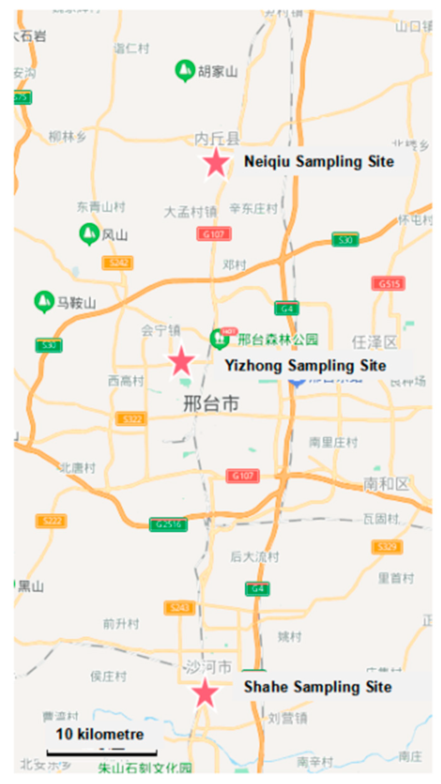
2.1.1. Sampling Position, Period, and Samples Collection

Xingtai is a typical industrial city, which has lots of glass, cement, and coking industries. Xingtai is also a northern city dominated by a north wind. Thus, many industrial plants are located in the south county of Shahe. In order to study the effects of transfer, emission, and weather conditions, three sampling sites were located in the main city (Yizhong Station, YZ) and the upwind (Neiqiu Station, NQ) and downwind Shahe Station, SH) direction of the main city during the autumn–winter season (Seen Figure 1). Sampling points all lay within 1.5–15 m from the ground in strict accordance with the provisions of the National Technical Specification for Layout of Ambient Air Quality Monitoring Points HJ 664-2013.
The sampling periods were two autumn–winter seasons which were from 15 October 2017 to 30 January 2018 and 15 October 2018 to 30 January 2019. Daily PM2.5 samples were collected continuously from 09:00 to 08:30 of the next day, and the sampling time was 23.5 h. Six hundred forty-eight film samples contained quartz and polypropylene were obtained for one autumn–winter season.
Two high-volume samplers (TH-150C, Tianhong Instrument Co. Ltd., Wuhan, China) were used to collect PM2.5 samples. Before the sampling process, the samplers were calibrated, the flow-rate range of the samplers was from 60 to 150 L/min (prolongable), with an accuracy of ±2.5%, and the relative error of the flow-rate of less than 2%. In this sampling process, the flow rate was set as 100 L·min−1; quartz and polypropylene films were loaded to capture PM2.5. After sampling, the filter samples were placed in the refrigerator at −4 °C for preservation.

2.1.2. Quality Assurance and Quality Control of Sampling

The quartz films were first calcined at 450 °C for 5 h in order to remove the organics and other impurities on the films. And then, the films were packed into aluminum foil papers and placed in a constant temperature and humidity chamber of 25 °C and 50 ± 5% relative humidity for 24 h. Then the films were sealed in film boxes at the temperature of −20 °C. Three blank films were reserved as the blank samples to correct the data of each sample in order to guarantee the accuracy and reliability of the analyzed data of the collected samples.

2.2. Chemical Components Analysis

2.2.1. Water Soluble Ions

Before analysis, polypropylene films were extracted ultrasonically by 20 mL of ultra-pure water for 20 min, and then water-soluble matters were filtrated and stored at 4 °C. Ion chromatography (Universal ics-90, Swiss) was used to analyze the inorganic ions, which included chloride (Cl), nitrate (NO3) and sulfate (SO42−), sodium (Na+), ammonium (NH4+), potassium (K+), magnesium (Mg2+), calcium (Ca2+), and fluoride (F).

2.2.2. Carbonaceous Species

A circular quartz filter with an area of 0.558 cm2 was used to determine organic carbon (OC) and elemental carbon (EC) concentrations by a thermal/optical carbon analyzer (Model 2008; Desert Research Institute, Reno, Nevada USA).
The background contamination was regularly monitored by blank tests, which were used to validate and correct the corresponding data. Calibration of the analyzer was done before and after sample analysis every day. The first sample was analyzed every ten samples again, and the precision should be less than 5%.

2.2.3. Inorganic Element

After the digestion process, metal components, such as Li, Be, Mg, Ti, V, Cr, Mn, Fe, Co, Ni, Cu, Zn, As, Se, Mo, Cd, Sn, Sb, Ba, Hg, Pb, Bi, Ca, K, Mg, Na, were determined using Inductively Coupled Plasma-Mass Spectrometry (7700 Series ICP-MS, Agilent Technologies Inc., PaloAlto CA, USA). In addition, the concentrations of Al and Si were determined by Inductively Coupled Plasma Atomic Emission Spectrometry (8300 ICP-AES, PerkinElmer company, Boston, Massachusetts, USA)

2.3. Data Analysis Method

2.3.1. Online Data Source

Air quality data were obtained from China’s air quality online monitoring and analysis platform (http://www/aqistudy.cn/historydata, accessed on 27 February 2021), and meteorological data were obtained from the National Oceanic and Atmospheric Administration (ftp://arlftp.arlhq.noaa.gov/pub/archives/gdas1/, accessed on 27 February 2021) which are all open-source database for research.

2.3.2. Analysis of Secondary Pollution

The secondary formation is an important reason for PM2.5 pollution. Sulfate and nitrate are the main productions by the secondary formation in PM2.5, and the components of which are related to the oxidation efficiency of SO2 and NO2. Usually, the secondary formation rates of SO2 and NO2 are characterized by SOR (sulfate oxidation rate) and NOR (nitrate oxidation rate), which can be calculated by the following equations:
SOR = (SO42−)/((SO42−) + (SO2))
NOR = (NO3)/((NO3) + (NO2))
where (SO42−) and (NO3) are concentrations in PM2.5, μg/m3; (SO2) and (NO2) are the concentrations of the gas phase, μg/m3.
Secondary organic carbon in the atmosphere is formed by photochemical reactions or gas-particle conversion of volatile and semi-volatile organic compounds. The degree of secondary carbon pollution can be characterized by indicators such as OC/EC and SOC/OC. The higher the ratio represents, the more serious secondary pollution. The secondary OC (SOC) concentrations were determined by the EC tracer method following Equations (3) and (4).
POC = EC × (OC/EC)min
SOC = OC − POC
where POC, SOC, and OC represent the estimated primary OC, secondary OC, and measured total OC, respectively. (OC/EC)min is the minimum OC/EC ratio in each sampling period.
Moreover, the value of the OC/EC ratio can also reflect the different combustion emission sources. It was suggested by the studies, the OC/EC ratio of vehicle exhaust emissions is 2.5–5.0, coal combustion is 5.0–10.5, wood-burning is 16.8–40.0, biomass burning is 7.7 [26,27,28].

2.3.3. Back Trajectory and Clustering Analysis

The 48 h backward trajectories of air mass during the pollution processes were investigated by the Hybrid Single Particle Lagrangian Integrated Trajectory (HYSPLIT) (http://ready.arl.noaa.gov/HYSPLIT.php, accessed on 27 February 2021) model developed by the National Oceanic and Atmosphere Administration (NOAA). The model started at a height of 100 m above ground level (AGL) with a time interval of one hour. Based on the results of the backward trajectory analysis, the trajectories and pollution concentrations were used to cluster analysis by MeteoInfoMap, which is an open-source geographic information system and scientific computing environment software.
Cluster analysis is an objective classification method to study multiple elements (or variables). It looks for a statistical quantity that can objectively reflect the distance relationship between samples and then divides samples into several categories according to the statistical quantity. The clustering method based on airflow trajectory is to group a large number of air flow tracks according to their spatial similarity (transmission velocity and direction). In this study, the Angle Distance algorithm provided by TrajStat software was used to cluster the airflow trajectory, and total spatial variance (TSV) was used to judge the classification quality. The principle is as follows: the TSV of the first several classification steps increases rapidly and then increases slowly. When the categories are divided to a certain number, TSV increases rapidly again, indicating that the merged categories are different. The classification merger is over, and the categories before the merger are the classification results. The average trajectories of these categories are the main flow trajectories of the target point in the analysis periods.

3. Results and Discussion

3.1. Mass Concentrations and Chemical Compositions of PM2.5

3.1.1. The Mean Values of Pollutants in the Two Autumn–Winter Seasons

The mean concentrations of PM2.5 and its major chemical components of the three sampling sites at Xingtai in the autumn–winter seasons of 2017–2018 and 2018–2019 are presented in Table 1, and the concentrations of other online air pollutants are also shown in this table. The mean concentrations of PM2.5, NO2, SO2, and O3 were 125.0, 60, 32, and 51 μg/m3 in the autumn–winter season of 2017–2018 and those were 112.1, 64, 31, and 40 μg/m3 in that of 2018–2019. Compared to the autumn–winter season of 2017–2018, the concentrations of PM2.5 and SO2 in that of 2018–2019 had a slight decrease. However, the concentrations of NO2 and O3 had a little increase. The air quality index (AQI) of the two autumn–winter seasons are shown in Figure 2, which shows that the study periods were dominated by polluted weather, specifically, the weather with AQI above 100 (light pollution) accounted for 65.7% and 64.8% in the two autumn-winter seasons, respectively.
Water-soluble inorganic ions are important components of PM2.5 which mainly include NO3, SO42−, NH4+, K+, Ca2+, and Cl [29,30]. These inorganic ions play an important role in the formation of PM2.5. On average, the most abundant water-soluble species in PM2.5 were ranked as follows: NO3 (20.7 μg/m3), SO42− (11.8 μg/m3), NH4+ (11.8 μg/m3), Cl (5.0 μg/m3), Ca2+ (1.6 μg/m3), and K+ (1.3 μg/m3) in 2017–2018, and NO3 (20.0 μg/m3), SO42− (9.6 μg/m3), NH4+ (9.1 μg/m3), Cl (4.0 μg/m3), Ca2+ (1.6 μg/m3), and K+ (0.8 μg/m3) in 2018–2019. Mean concentrations of SNA (Secondary inorganic aerosol, which is the sum of SO42−, NO3, and NH4+) were 44.3 μg/m3 in 2017–2018 and 38.7 μg/m3 in 2018–2019, contributing 35.4% and 34.5% in PM2.5 mass. It can be concluded that in two autumn–winter seasons, the mass concentration values of SO42− and NH4+ were all similar, which suggested that (NH4)2SO4 was the main formation of SO42− and NH4+ in PM2.5. Furthermore, it also can be seen that the mass concentration of NO3 was more than that of SO42−, which suggests that the pollution style of Xingtai was of nitrate, indicating that the usage control of carbon reduced SO2 emissions effectively, however, NOx emissions of vehicles and gas-fired boilers should be controlled further.
Carbonaceous species, which mainly include EC and OC, were found to contribute significantly to the formation of fine particles. EC is one of the main light-absorbing species in fine particles and also is the gas to particle reaction medium for SO2 and NOx [31]. Moreover, EC is a good indicator of primary anthropogenic pollutants [28]. The source of OC is more complex. Besides the primary emissions from industrial production, fuel combustion, and natural sources, there is secondary organic carbon (SOC) produced by photochemical reactions of gaseous precursors in the atmosphere [32]. The mean concentrations of OC and EC were 26.6 and 18.1 μg/m3 in the autumn–winter season of 2017–2018, and those were 19.0 and 7.5 μg/m3 in that of 2018–2019. The contributions of OC and EC in the PM2.5 mass concentrations were 21.3% and 18.1% in the autumn–winter season of 2017–2018, and those were 16.9% and 6.7% in that of 2018–2019. The concentration and ratio of EC all had an obvious decline in 2018–2019 compared with 2017–2018 in the study period, suggesting that the direct emission of fossil fuel and incomplete combustion of biomass from pollution sources [33] were reducing. It was known that the plan of Xingtai’s comprehensive control of air pollution had been issued, which controlled the scattered coal burning for civil use effectively. The measures of the plan included a ban on burning scattered coal, connecting the urban heating network, carrying out central heating or clean heating in all county areas. Through these measures, control of the combustion of scattered coal at Xingtai in the autumn-winter season of 2018–2019 achieved initial success.
Usually, the OC/EC values are often used to determine whether secondary pollution occurs. If the OC/EC values exceed 2.0, there is secondary pollution [34]. Through calculation, the average OC/EC value in the autumn–winter season of 2017–2018 was 2.1, and that of 2018–2019 was 2.3. Therefore, secondary pollution more likely happened in the autumn–winter season of 2017–2018 and 2018–2019. Moreover, the concentrations of SOC could also reflect the level of secondary pollution and were also calculated. The concentration of SOC were 1.3 and 6.9 μg/m3 in the study period of 2017–2018 and 2018–2019, respectively, accounting for 4.9% and 38.1% in OC, respectively, suggesting that the chemical conversion process had more effects on the formation of PM2.5 in the autumn–winter season of 2018–2019 compared that of 2017–2018. On the other side, it could also be concluded that the atmospheric oxidation of 2018–2019 was higher than that of 2017–2018 at Xingtai.
In this study, the OC/EC ratios were 2.1 and 2.3 in the autumn–winter season of 2017–2018 and 2018–2019, respectively. Thus, the main combustion source was vehicle exhaust. OC/EC ratios of 2018–2019 have increased which were attributed to the increase in atmospheric oxidation. NOx was the main oxidizing substance in the atmosphere, and NOx released by vehicle emissions contributed significantly, so more efforts should be directed toward vehicle NOx emissions.

3.1.2. The Mean Values of the Three Sampling Sites in the Autumn–Winter Seasons

Table 1 shows the mass concentrations of PM2.5 and its major chemical components in the three monitoring stations. Neiqiu and Shahe are two counties located in the upwind and downwind directions of the main urban city of Xingtai during the autumn–winter season. Among the three sampling sites, Shahe is an important industry county, which had many glass, ceramics, and coking industries. In general, as seen in Table 1, compared to the year 2017–2018, the mass concentration of PM2.5 in the three sampling sites of YZ, NQ, and SH all decreased by 13.7%, 4.3%, and 12.6%, respectively, in the year 2018–2019. However, both in the two autumn–winter seasons, the mass concentration of PM2.5 in SH was the highest, which could be attributed to more agminated factories.
Table 1 also shows that all the PM2.5 components have a similar pattern. The average concentrations of the total water-soluble ions at YZ, NQ, and SH were 52.7, 48.3, and 55.6 μg/m3 in the autumn–winter season of 2017–2018, and those were 42.2, 47.4, and 45.5 μg/m3 in that of 2018–2019, the decrease ratios were 19.9%, 1.9%, and 18.2%, respectively. Moreover, the decreasing rates of ion concentrations were calculated, as for SNA, and the decrease ratios of YZ and SH were all larger than those of NQ. It can be speculated that NQ was easily affected by the pollution transport. Moreover, it was to note that the concentration of NO3 was increased at NQ, which all suggested that nitrate pollution was a severe air pollution issue.
As seen in Table 1, the concentrations of OC in the three sampling sites were 17.5, 16.3, and 20.4 μg/m3 in the autumn–winter season of 2017–2018 and those were 15.3, 21.8, and 20.0 μg/m3 in 2018–2019. Compared to the autumn–winter season of 2017–2018, OC and EC values of YZ and SH all had a slight decrease in that of 2018–2019. However, as for NQ, OC value was increased, and EC value kept steady. It could be concluded that in autumn–winter seasons, the additional fossil fuels clearly lead to an increase in OC emissions, and under the unfavorable meteorological conditions, the higher concentrations of OC may be precursors and attributed to the increase in secondary formations [35,36].
The mass concentrations of Cl, K+, and Ca2+ were relatively low in the total water-soluble inorganic ions. K+ could be used to trace biomass emissions and fireworks emissions [37]. It was suggested that the mass concentration of K+ in the autumn–winter season of 2018–2019 was lower than that of 2017–2018. It was known that the Administrative Measures of Xingtai City on Banning Open Burning (Trial) was released in 2018–2019, and biomass burning has been further controlled effectively so that the mass concentration of K+ of the three sampling sites all had decreased. Chloride ions (Cl) mainly come from coal combustion [38], and the mass concentrations of Cl in YZ and SH all decreased in the autumn–winter season of 2017–2018 compared to those of 2018–2019, suggesting that the coal-fired combustion was further controlled in 2018–2019 compared to 2017–2018. Calcium ions (Ca2+) mainly come from crustal-derived ions and are indicators of soil-related sources [39]. As shown in Table 1, the concentration of Ca2+ in the two autumn–winter seasons were similar, suggesting that those seasons suffered a similar sandstorm situation.

3.2. Chemical Components Analysis at Different PM2.5 Concentration Levels

Among the normal six-item air pollutants, CO is not an active photochemical and has a chemical life of about several months. In a short period, CO can be regarded as an inert pollution tracer, mainly controlled by meteorological parameters [40,41,42,43]. The ratios of PM2.5/CO, SO2/CO, NO2/CO, and O3/CO were calculated under different AQI levels to understand the relative contribution of the chemical processes to PM2.5.
It can be seen in Table 2, the concentration ratios of PM2.5/CO and SO2/CO did not change obviously with different PM2.5 concentration levels in both years. However, the ratio of NO2/CO and O3/CO all decreased with an increase in PM2.5 concentration levels, suggesting that on heavy pollution days, the chemical conversion processes of the pollutants happened. NO2 acted as reactants to produce the chemical reactions and forming more sulfates and nitrates, and O3 formation process was restrained. It can be seen in Table 2 that the concentration ratio of O3/CO had an obvious decrease with the increase in the concentration ratio of PM2.5/CO. Thus, it can be speculated that on heavy pollution days, the concentration of PM2.5 and O3 had a negative correlation because of the chemical conversion processes, and O3 could act as an important oxidizing agent. On the other hand, photochemical production of O3 decreased during the occurrences of haze events which also attribute to the decrease in O3/CO.
In order to analyze the chemical components of PM2.5 at different pollution levels, in this study, we further split the days into five levels according to the concentration of PM2.5 as shown in Figure 3. The columns presented the average concentrations of PM2.5 at their respective pollution levels. It can be seen in Figure 3, the concentration of Ca2+ and K+ are at low levels, suggesting that sand storms and biomass burning had fewer contributions to the concentration of PM2.5. The concentration of Cl stays stable with the increase in pollution level, indicating that the contribution of coal combustion to the air pollution did not further increase with the deepening of the pollution. It is to note in Figure 3, the concentration variation trends of SO42− and NH4+ were similar, which increase with the increase in PM2.5 concentration. It was indicated that (NH4)2SO4 was the important component of PM2.5. Considering that SO42− also mainly come from coal combustion, the emission level of coal combustion did not increase due to the stable level of Cl concentration. Thus, it could be concluded that the atmospheric oxidation increased with the deepening of pollution and making the secondary conversion level increase. NO3 was the main water-soluble ion of PM2.5, and the pollution style of the autumn–winter season in Xingtai was nitrate dominant. Moreover, the concentration of NO3– increased sharply when the concentration of PM2.5 was higher than 150 μg/m3, which also proved that the secondary conversion process was enhanced at the heavy pollution weather.
The concentrations of EC, OC, and the concentration ratios of OC/EC, NO3/SO42− at different concentration levels of PM2.5 in the two autumn–winter seasons are shown in Figure 4. With the increase in the PM2.5 concentration levels, the concentrations of OC and EC all increased. Though the concentrations of OC and EC in the autumn–winter season of 2018–2019 were lower than those of 2017–2018, the concentration ratio of OC/EC in 2018–2019 was higher than that in 2017–2018, indicating that though the total carbon decreased, the secondary conversion rate increased. OC/EC level was higher at the high concentration level of PM2.5, suggesting that chemical conversion was enhanced during high pollution weather. The concentration ratios of NO3/SO42− are also shown in Figure 4, which indicates that the concentration ratios of NO3/SO42− in the autumn–winter season of 2018–2019 were higher than those of 2017–2018, which also proves the importance of NOx pollution control.

3.3. Impacts of Meteorological Parameters and Secondary Formation

Fine particulate matter (PM2.5) and O3 are the main substances causing air pollution in China, and it was testified that the combined pollution of PM2.5 and O3 were affected by the meteorological parameters and secondary formation [43,44,45].

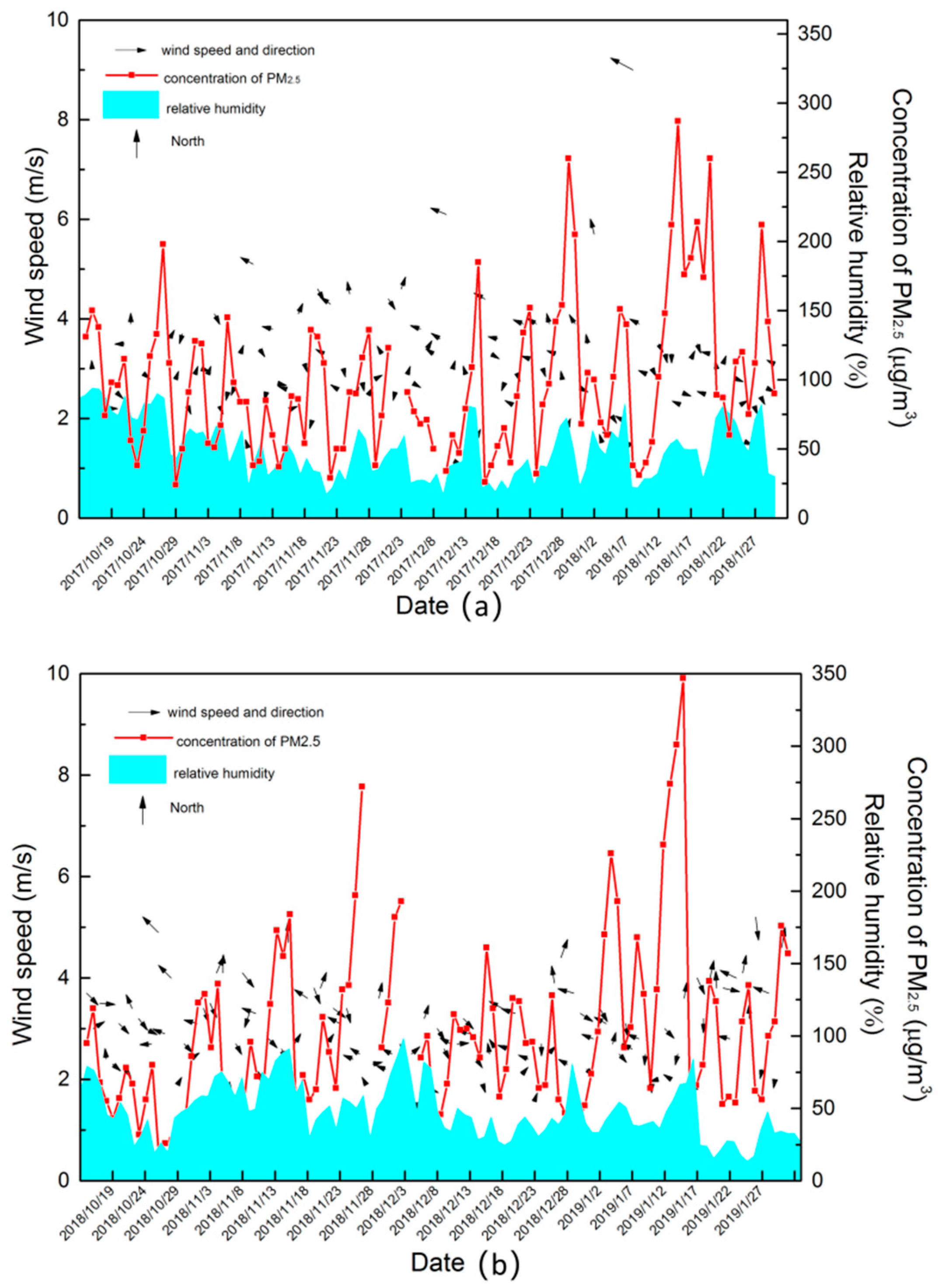
3.3.1. Impacts of Meteorological Parameters on the Formation of PM2.5 and O3

The online concentrations of PM2.5 and O3 in the two autumn–winter seasons are shown in Figure 5, the average online concentration of PM2.5 and O3 were 100 and 51 μg/m3 at the autumn–winter season of 2017–2018, and those were 100 and 40 μg/m3 in the autumn–winter season of 2018–2019. Thus, it could be concluded that PM2.5 was the main air pollutant in the autumn–winter season in Xingtai. As shown in Figure 5, the concentrations of PM2.5 and O3 had different variation tendencies. Thus, it is speculated that the meteorological parameters and secondary formation had different effects on the formation of PM2.5 and O3.
The meteorological parameters of the two autumn–winter seasons are shown in Figure 6. The average wind speed, temperature, and relative humidity were 3.0 m/s, 4 °C, and 49.9% in the autumn–winter season of 2017–2018, and those were 2.9 m/s, 4 °C, and 47.7% in the autumn–winter season of 2018–2019. Thus, it could be concluded that the meteorological conditions of the two autumn–winter seasons were similar, which all had low wind speed and high relative humidity. It could be concluded from Figure 6, high humidity and low wind speed could promote the formation of air pollution. It was because in the autumn–winter seasons, low temperature and low wind speed caused the accumulation of pollution. Moreover, the high relative humidity increased the reaction rate of the heterogeneous and liquid phase reactions, which was in favor of the pollution process. In addition, it also can be seen in Figure 6, that wind has obvious effects on removing pollution.
In order to explore the correlations between the concentrations of PM2.5, O3, and the meteorological parameters, Kendall’s Tau coefficients were calculated, and the calculation results are shown in Table 3. It can be seen in Table 3, both PM2.5 and O3 had a weak correlation with the average air pressure. It can be seen that wind speed had a positive correlation with the concentration of O3 and had a negative correlation with the concentration of PM2.5. Thus, it is suggested that wind had the opposite effects on the formation of PM2.5 and O3. The formation of O3 mainly depended on the secondary formation of the emission pollutants, and it was speculated that wind could increase the disturbance of the chemical matters in the atmosphere, further increase the reactants contacting probability of O3. As for PM2.5, nucleation is the main step for the formation of PM2.5. However, high wind speed increases the disturbance of airflow, inhibiting the forming of the nucleus.
It also can be seen in Table 3, the temperature had a higher Kendall’s Tau coefficient with the concentration of O3 than that of PM2.5, suggesting that O3 is affected more easily by temperature. Higher temperatures were beneficial for the photochemical reaction to form O3, and went against the coagulating effects for forming PM2.5. The average relative humidity also had a positive correlation with the concentration of PM2.5, which demonstrated that water played an important role in the formation of PM2.5, because water molecules are an important component in the nucleation process.

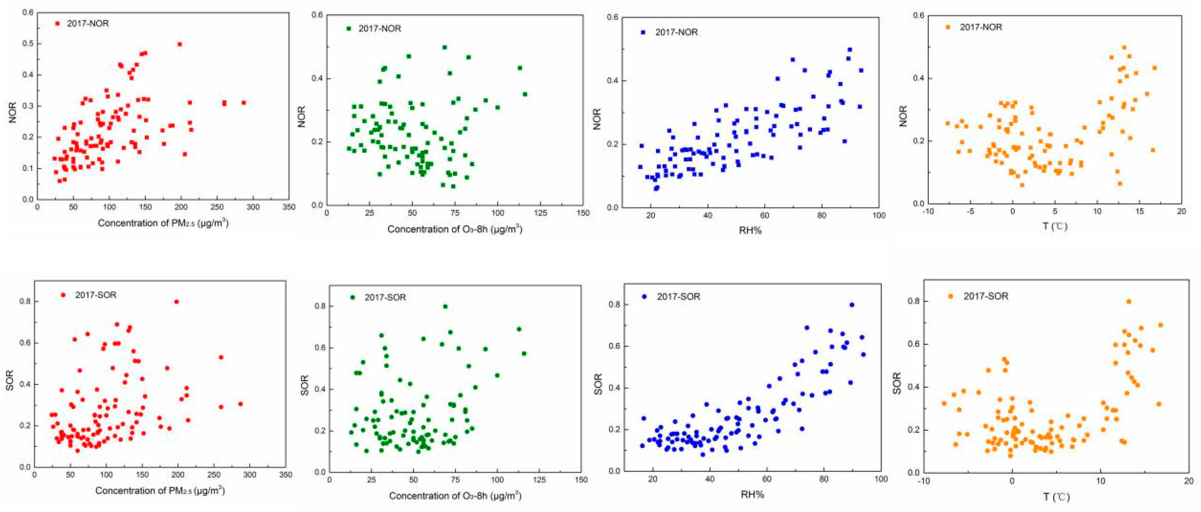
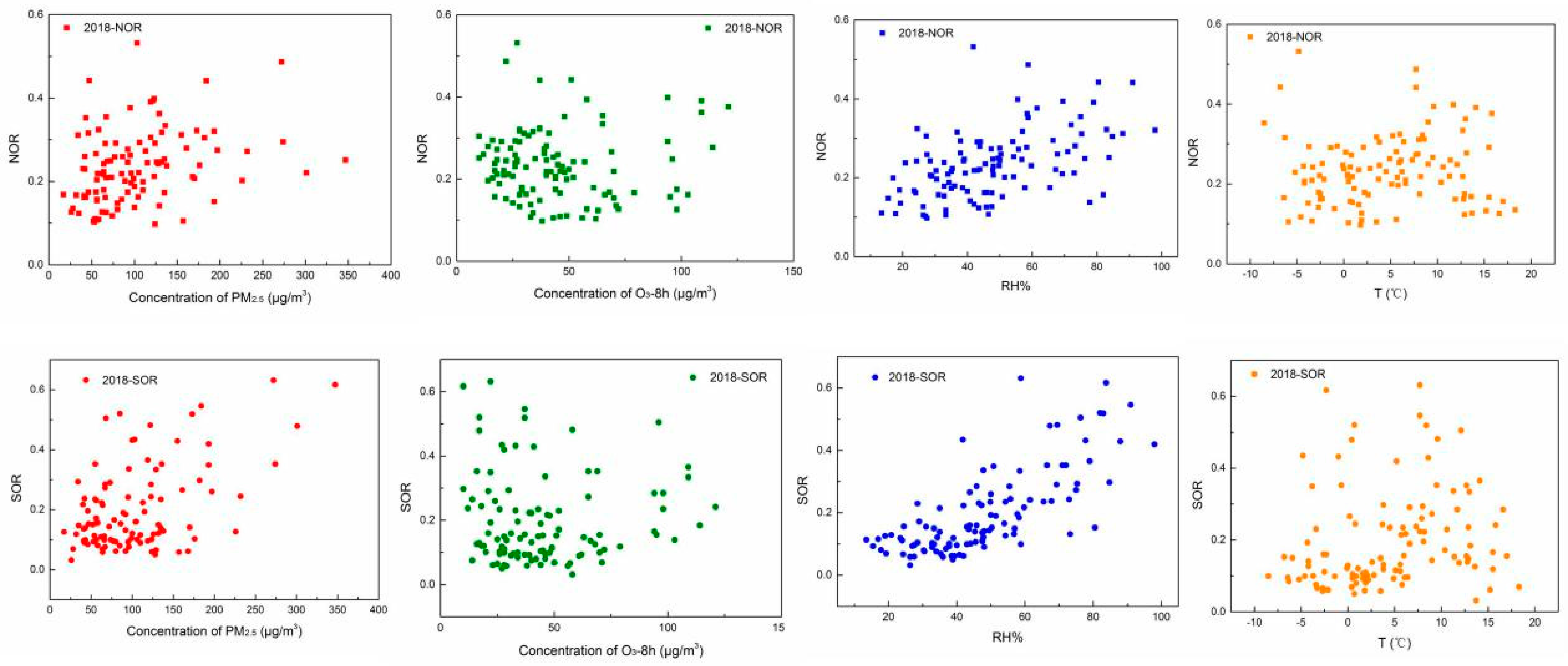
3.3.2. The Influence Factor of Secondary Aerosols in the Autumn–Winter Seasons

NOR and SOR are the indicators of secondary aerosols in the atmosphere. The average values of NOR and SOR were 0.22 and 0.27 in the autumn–winter season of 2017–2018 and those were 0.23 and 0.20 in that of 2018–2019, and the values of NOR in the two autumn–winter seasons were similar, the value of SOR was higher in the autumn–winter season of 2017–2018 compared to that of 2018–2019. According to Table 3, the temperature and relative humidity have more effects on the formation of PM2.5 and O3, thus in order to study the relationships between the secondary aerosols and PM2.5 concentration, O3 concentration, relative humidity, and temperature, the correlations of them at the two autumn-winter seasons are shown in Figure 7 and Figure 8, respectively. Kendall’s tau coefficient between NOR, SOR, and the temperature, relative humidity concentration of PM2.5, O3 are shown in Table 4.
As shown in Figure 7 and Figure 8, the relationships of NOR and SOR against the temperature present a “U” shape. The values of NOR and SOR show small values at a temperature around 4 °C. It was speculated that the oxidation processes of SO2 and NO2 could be conducted either in the gaseous phase of the atmosphere or the interface between the gas phase and particle phase of the nuclei, and higher temperature benefited oxidation reaction in the gas phase. However, lower temperature benefited the nucleation process of the pollutants in the atmosphere, which provided larger surface areas for the inter-phase oxidation reactions. Thus, when the temperature was around 4 °C, gas-phase oxidation and gas-solid-phase oxidation were also not promoted, and NOR and SOR were relatively low.
It can be seen in Figure 7 and Figure 8, the relative humidity (RH) plays an important role in the formation of nitrates and sulfates. Thus, NOR and SOR increase with the increase in RH. It was suggested by the previous studies, RH could promote the formation of NO3– and SO42− in two ways: one way was that original sulfate and nitrate could adsorb water to enlarge the particles’ surfaces, and lager particle surfaces also promote the heterogeneous reaction to form NO3 and SO42−; the other way was that higher RH could decrease the viscosity of the surface of the particles, which increased the conversion rate of gas precursors to particulate matter kinetically, resulting in more pollutant converting to particulate state, which promotes heterogeneous reactions [46].
By calculation, Kendall’s tau coefficients were 0.440 and 0.295 for NOR and SOR to the concentration of PM2.5, respectively in the autumn–winter season of 2017–2018, and those were 0.252 and 0.205 in that of 2018–2019 (As seen in Table 4). NOR and SOR showed a positive correlation with the concentration of PM2.5, indicating that the secondary formation contributes to the formation of PM2.5, and the promotion effects were not very strong, which suggested that except for the secondary formation, many other factors all affected the formation of PM2.5 pollution. The Kendall’s tau coefficients were −0.101 and 0.082 for NOR and SOR to the concentration of O3, respectively in the autumn–winter season of 2017–2018, and those were −0.076 and −0.032 in the autumn–winter season of 2018–2019. It could be concluded that the concentration of O3 had a poor correlation with NOR and SOR. Thus, it was speculated the secondary formation process of SO42 and NO3 had minor effects on the formation of O3. The photochemical reaction of O3 and secondary formation of SO42, NO3 may be controlled by different main factors. Humidity and temperature had a positive effect on the formation of SOR and NOR. It was suggested that higher temperatures and a humid environment could accelerate the chemical reaction.

3.4. Identification of Potential Transported Sources

Regional transport is another important reason for the formation of air pollution. Thus, the meteorological conditions and transport of PM2.5 and O3 during the pollution processes were studied. As shown in Table 5, there were six pollution processes during the sampling periods in 2017–2018, and the information on the pollution processes is shown in Table 5.
The wind roses of the six pollution periods and the whole sampling period at the autumn–winter season of 2017–2018 are shown in Figure 9. It can be seen in Figure 9A, the predominant wind direction in the autumn–winter season was northwest. However, the predominant wind directions during the pollution periods were southeast and north-east directions, as shown in Figure 9B. Thus, it can be suggested that the pollution of Xingtai is mainly affected by the east cities at Shandong and Hebei province.
The clustering analysis of the backward flow trajectory of the six typical pollution processes was conducted, and the clustering results are shown in Figure 10. It can be seen that all the pollution processes were affected by the airflow coming from the east. In order to make clear the pollution concentrations in each airflow trajectory, three pollution processes were selected, and the pollutants (O3 and PM2.5) contribution ratio is shown in Figure 11. As shown in Figure 11, O3 and PM2.5 usually have different main transport paths. The main PM2.5 transport paths of the pollution processes I, III, and VI were path 2, path 2, and path 3, respectively; however, the main O3 transport paths of those pollution processes were path 1, path 4, and path 3, respectively. It could be concluded that the main pollution transport paths of O3 in Xingtai were all from the east. Thus, O3 pollution of Xingtai in winter was easily affected by Shandong province except for the Beijing–Tianjin–Hebei area. As seen in Figure 9B, the predominant wind direction in Xingtai is northwest. However, among the main pollution transport paths of the pollutants, only in pollution process I, the main PM2.5 pollution was transported from the northwest. Thus, it was suggested that the pollution emissions of the cities located in the east of Xingtai had more effects on the pollution processes of Xingtai. It can be considered that more focus should be paid to the industrial restructuring and energy structure optimization of the cities at the east of Beijing–Tianjin–Hebei area to control PM2.5 and O3 pollution synergistically.

4. Conclusions

Xingtai city, located at the south part of the Beijing–Tianjin–Hebei area, east side of the Taihang mountains, which has developed secondary industry leading to large amounts of local emissions. In addition, Xingtai city is affected by the pollution transport obviously, and local pollutants are hard to diffuse, which is a typical industry city with bad pollutant diffusion conditions. This study made a comprehensive analysis of air pollution from the aspects of pollutants emission, meteorology conditions, secondary formation, and pollutants transport, respectively, in two autumn–winter seasons of 2017–2018 and 2018–2019 at Xingtai. Moreover, the effects of the secondary formation and meteorological conditions on the combined pollution of PM2.5 and O3 were explored due to the fact that combined pollution controlling was a new challenge in China. The rules of the relationship between PM2.5, O3, and other factors were studied, and air trajectories and pollutant concentrations were clustered to find different transmission paths of PM2.5 and O3. The specific research conclusions are shown below:
  • PM2.5 concentration had a slight decrease in the autumn–winter season of 2018–2019 compared to that of 2017–2018, the concentration of EC, SO42−, NH4+, Cl, and K+ all decreased, which could attribute to carrying out the central and clean heating policies and control of biomass burning policy at Xingtai in 2018–2019. However, the secondary formation rates increased obviously in the autumn–winter season and the concentration of NO3 kept steady. In addition, the average concentration of NO2 also increased. Thus, NOx control was an important pollutant control work in the future.
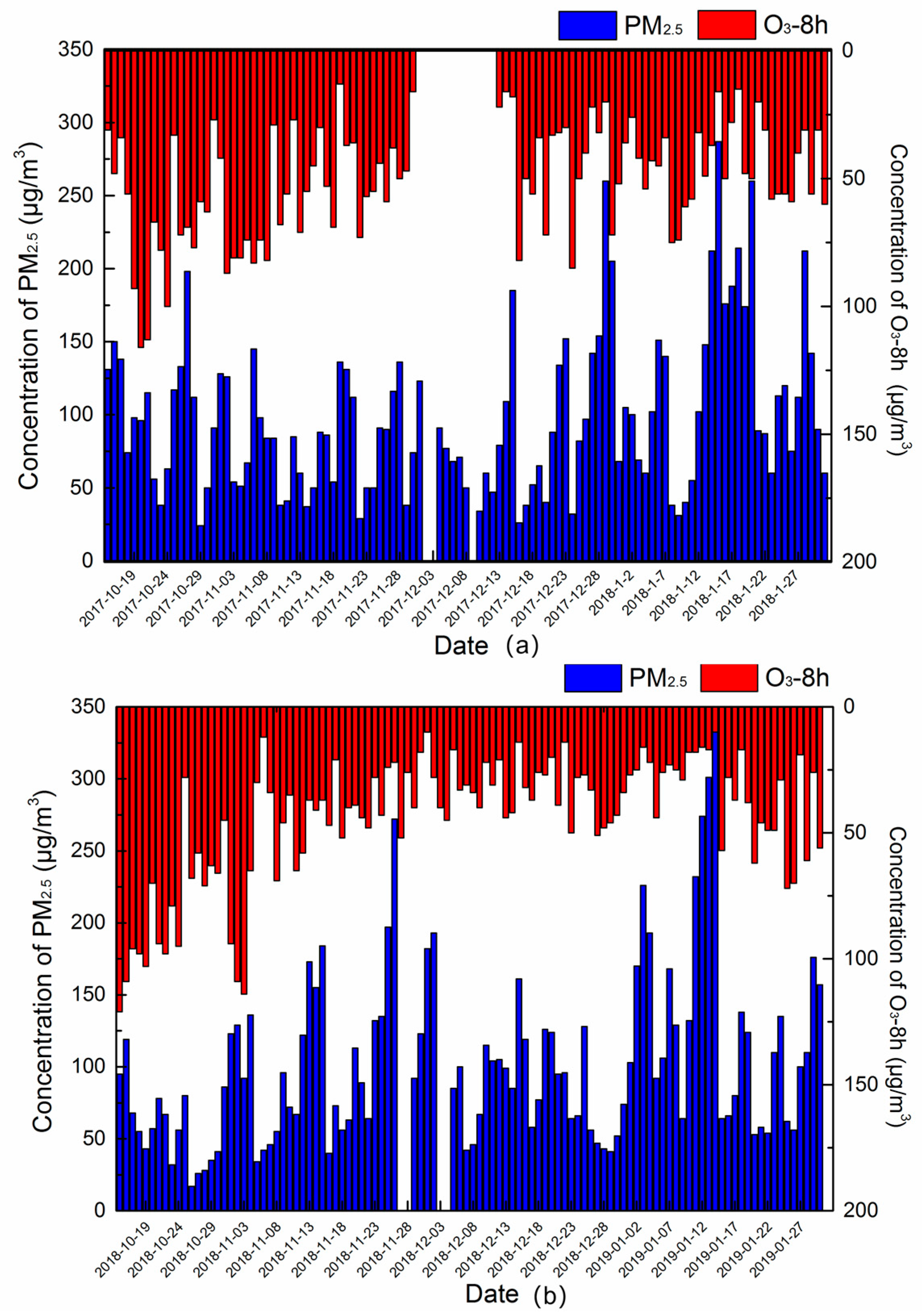
  • The formation of O3 and PM2.5 all affected by the secondary formation and meteorological conditions, but the impact effects of the factors were not the same. With the increase in PM2.5 pollution levels, the secondary formation increased, and O3 was consumed. Furthermore, the study of correlation suggested that the concentrations of O3 and PM2.5 were easily affected by the temperature and relative humidity, respectively.
  • The increase in the relative humidity benefited the formation of SOR and NOR. The relationships of NOR and SOR against temperature present a “U” shape. The values of NOR and SOR showed small values at a temperature of around 4 °C because gas-phase oxidation and gas-solid-phase oxidation were also not promoted at this temperature, thus decreased the secondary formation.
  • The cluster of air trajectories and concentrations of PM2.5 and O3 showed that the pollution of Xingtai is mainly affected by the east cities located in the Shandong and Hebei province. The east route was the main transport route for O3 and PM2.5. However, the concentration of PM2.5 was also affected by the airflow coming from the northwest.

Author Contributions

Conceptualization, S.W.; methodology, J.Z. and H.W.; data analysis and discussion of the results, H.W.; sample collection and data determination and validation, H.W. and H.L.; writing—original draft preparation, H.W.; writing—review and editing, S.W. and H.L. All authors have read and agreed to the published version of the manuscript.

Funding

This work was supported by the National Key Research and Development Program (2019YFC0214200).

Institutional Review Board Statement

Not applicable.

Informed Consent Statement

Not applicable.

Data Availability Statement

Not applicable.

Acknowledgments

The authors would like to thank the Bureau of Ecology and Environment of Xingtai for administrative support of this study and thank the Environmental Monitor Center of Xingtai for technical support of this study.

Conflicts of Interest

The authors declare no conflict of interest.

References

  1. Yuling, H.; Shigong, W. Formation mechanism of a severe air pollution event: A case study in the Sichuan Basin, Southwest China. Atmos. Environ. 2021, 246, 118135. [Google Scholar] [CrossRef]
  2. Jianjun, H.; Sunling, G.; Ye, Y.; Lijuan, Y.; Lin, W.; Hongjun, M.; Congbo, S.; Suping, Z.; Hongli, L.; Xiaoyu, L.; et al. Air pollution characteristics and their relation to meteorological conditions during 2014–2015 in major Chinese cities. Environ. Pollut. 2017, 223, 484–496. [Google Scholar]
  3. Chen, Y.; Xie, S. Spatiotemporal pattern and regional characteristics of visibility in China during 1976–2010. Chin. Sci. Bull. 2014, 59, 3054–3065. [Google Scholar] [CrossRef]
  4. Fanglin, C.; Zhongfei, C. Cost of economic growth: Air pollution and health expenditure. Sci. Total. Environ. 2021, 755, 142543. [Google Scholar] [CrossRef]
  5. Hawawu, H.; Mansour, S.; Masud, Y.; Mohammad, S.H.; Tanko, M.; Akbar, F. Fuel type use and risk of respiratory symptoms: A cohort study of infants in the Northern region of Ghana. Sci. Total. Environ. 2021, 755, 142501. [Google Scholar] [CrossRef]
  6. Wenxing, W.; Tao, W. On acid rain formation in China. Atmos. Environ. 1996, 30, 4091–4093. [Google Scholar] [CrossRef]
  7. Qingqing, H.; Ming, Z.; Yimeng, S.; Bo, H. Spatiotemporal assessment of PM2.5 concentrations and exposure in China from 2013 to 2017 using satellite-derived data. J. Clean. Prod. 2021, 286, 164965. [Google Scholar] [CrossRef]
  8. Fangyuan, W.; Xionghui, Q.; Jingyuan, C.; Lin, P.; Nannan, Z.; Yulong, Y.; Rumei, L. Policy-driven changes in the health risk of PM2.5 and O3 exposure in China during 2013–2018. Sci. Total. Environ. 2021, 757, 143775. [Google Scholar] [CrossRef]
  9. Chong, J.; Reshmita, N.; Lev, L.; Dewang, W. Integrating ecosystem services into effectiveness assessment of ecological restoration program in northern China’s arid areas: Insights from the Beijing-Tianjin Sandstorm Source Region. Land Use Policy 2018, 75, 201–214. [Google Scholar] [CrossRef]
  10. Qiang, J.; Xinyue, F.; Bo, W.; Aidang, S. Spatio-temporal variations of PM2.5 emission in China from 2005 to 2014. Chemosphere 2017, 183, 429–436. [Google Scholar] [CrossRef]
  11. Pengfei, W.; Hao, G.; Jian, H.; Sri, H.K.; Qi, Y.; Hongliang, Z. Responses of PM2.5 and O3 concentrations to changes of meteorology and emissions in China. Sic. Total. Environ. 2019, 662, 297–306. [Google Scholar]
  12. Lei, C.; Jia, Z.; Yang, Y.; Xu, Y. Meteorological influences on PM2.5 and O3 trends and associated health burden since China’s clean air actions. Sci. Total. Environ. 2020, 744, 140837. [Google Scholar] [CrossRef]
  13. Gao, Y.; Zhang, M.; Liu, Z.; Wang, L.; Xia, X.; Tao, M.; Zhu, L. Modeling the feedback between aerosol and meteorological variables in the atmospheric boundary layer during a severe fog–haze event over the North China Plain. Atmos. Chem. Phys. 2015, 15, 4279–4295. [Google Scholar] [CrossRef] [Green Version]
  14. Ziyue, C.; Danlu, C.; Mei, P.K.; Bin, C.; Bingbo, G.; Yan, Z.; Ruiyuan, L.; Bing, X. The control of anthropogenic emissions contributed to 80% of the decrease in PM2.5 concentrations in Beijing from 2013 to 2017. Atmos. Chem. Phys. 2019, 19, 13519–13533. [Google Scholar] [CrossRef] [Green Version]
  15. Yang, Y.; Lynn, M.R.; Sijia, L.; Hong, L.; Jianping, G.; Ying, L.; Balwinder, S.; Steven, J.G. Dust-wind interactions can intensify aerosol pollution over eastern China. Nat. Commun. 2017, 8, 15333. [Google Scholar] [CrossRef] [PubMed]
  16. Zhengtai, Z.; Kaicun, W. Stilling and recovery of the surface wind speed based on observation, reanalysis, and geostrophic wind theory over China from 1960 to 2017. J. Clim. 2020, 33, 3989–4008. [Google Scholar] [CrossRef] [Green Version]
  17. Nadine, U.; Drew, T.S.; Dorothy, K.; Markus, A.; Janusz, C.; David, G.S. Influences of man-made emissions and climate changes on tropospheric ozone, methane, and sulfate at 2030 from a broad range of possible futures. J. Geophy. Res. 2006, 111, D12. [Google Scholar] [CrossRef]
  18. Isaksen, I.S.A.; Granier, C.; Myhre, G.; Berntsen, T.K.; Dalsøren, S.B.; Gauss, M.; Klimont, Z.; Benestad, R.; Bousquet, P.; Colins, W.; et al. Increase of ozone concentrations, its temperature sensitivity and the precursor factor in South China. Atmos. Environ. 2009, 43, 5138–5192. [Google Scholar] [CrossRef]
  19. Pavan, N.R.; Peter, J.A. Sensitivity of global tropospheric ozone and fine particulate matter concentrations to climate change. J. Geophys. Res. 2006, 111, D24103. [Google Scholar] [CrossRef]
  20. Xiaoyan, W.; Robert, E.D.; Liangyuan, S.; Chunlüe, Z.; Kaicun, W. PM2.5 pollution in China and how it has been exacerbated by terrain and meteorological conditions. Bull. Am. Meteorol. Soc. 2018, 99, 105–119. [Google Scholar] [CrossRef]
  21. Yuzhu, X.; Zirui, L.; Tianxue, W.; Xiaojuan, H.; Jingyuan, L.; Guiqian, T.; Yang, Y.; Xingru, L.; Rongrong, S.; Bo, H.; et al. Characteristics of chemical composition and seasonal variations of PM2.5 in Shijiazhuang, China: Impact of primary emissions and secondary formation. Sci. Total Environ. 2019, 677, 215–229. [Google Scholar] [CrossRef]
  22. Yuesi, W.; Li, Y.; Lili, W.; Zirui, L.; Dongsheng, J.; Guiqian, T.; Junke, Z.; Yang, S.; Bo, H.; Jinyuan, X. Mechanism for the formation of the January 2013 heavy haze pollution episode over central and eastern China. Sci. China Earth Sci. 2013, 57, 14–25. [Google Scholar] [CrossRef]
  23. Zhaofeng, T.; Keding, L.; Meiqing, J.; Rong, S.; Huabin, D.; Limin, Z.; Shaodong, X.; Qinwen, T.; Yuanhang, Z. Exploring ozone pollution in Chengdu, southwestern China: A case study from radical chemistry to O3-VOC-NOx sensitivity. Sci. Total Environ. 2018, 636, 775–786. [Google Scholar] [CrossRef]
  24. Renyi, Z.; Gehui, W.; Song, G.; Misti, L.Z.; Qi, Y.; Yun, L.; Weigang, W.; Min, H.; Yuan, W. Formation of urban fine particulate matter. Chem. Rev. 2015, 115, 3803–3855. [Google Scholar] [CrossRef]
  25. Huijia, Z.; Huizheng, C.; Lei, Z.; Ke, G.; Yanjun, M.; Yaqiang, W.; Hong, W.; Yu, Z.; Xiaoye, Z. How aerosol transport from the North China plain contributes to air quality in northeast China. Sci. Total Environ. 2020, 738, 139555. [Google Scholar] [CrossRef]
  26. Charles, L.B.; Philip, M.R.; Shelley, J.T.; Steve, D.Z.; John, H.S. The use of ambient measurements to identify which precursor species limit aerosol nitrate formation. J. Air Waste Manag. Assoc. 2011, 50, 2073–2084. [Google Scholar] [CrossRef] [Green Version]
  27. Yanlin, Z.; Jun, L.; Gan, Z.; Peter, Z.; Rujin, H.; Jianhui, T.; Lukas, W.; André, S.H.P.; Sönke, S. Radiocarbon-based source apportionment of carbonaceous aerosols at a regional background site on Hainan Island, South China. Environ. Sci. Technol. 2014, 48, 2651–2659. [Google Scholar] [CrossRef]
  28. Chen, Y.; Zhi, G.; Feng, Y.; Fu, J.; Feng, J.; Sheng, G.; Simoneit, B.R.T. Measurements of emission factors for primary carbonaceous particles from residential raw-coal combustion in China. Geophys. Res. Lett. 2006, 33. [Google Scholar] [CrossRef]
  29. Baoqing, W.; Zhenzhen, T.; Ningning, C.; Honghong, N. The characteristics and sources apportionment of water-soluble ions of PM2.5 in suburb Tangshan, China. Urban Clim. 2021, 35, 100742. [Google Scholar] [CrossRef]
  30. Dan, W.; Shao-Long, L.; Huan-Qiang, Y.; Rong-Guang, D.; Jun-Rong, X.; Bing, Q.; Gang, L.; Feng-Ying, L.; Meng, Y.; Xin-Lei, G. Pollution characteristics and light extinction contribution of water-soluble ions of PM2.5 in Hangzhou. Environ. Sci. 2017, 38, 2656–2666. [Google Scholar] [CrossRef]
  31. Mo, D.; Guoshun, Z.; Xinxin, L.; Hairong, T.; Yahui, Z. The characteristics of carbonaceous species and their sources in PM2.5 in Beijing. Atmos. Environ. 2004, 38, 3443–3452. [Google Scholar] [CrossRef]
  32. Di, Y.; Qi, Z.; Changtan, J.; Jun, C.; Xiaoxing, M. Characteristics of elemental carbon and organic carbon in PM10 during spring and autumn in Chongqing, China. China Part. 2007, 5, 255–260. [Google Scholar] [CrossRef]
  33. Meng, C.C.; Wang, L.T.; Zhang, F.F.; Wei, Z.; Ma, S.M.; Ma, X.; Yang, J. Characteristics of concentrations and water-soluble inorganic ions in PM2.5 in Handan City, Hebei province, China. Atmos. Res. 2016, 171, 133–146. [Google Scholar] [CrossRef]
  34. Yuanxun, Z.; Min, S.; Yuanhang, Z.; Limin, Z.; Lingyan, H.; Bin, Z.; Yongjie, W.; Xianlei, Z. Source profiles of particulate organic matters emitted from cereal straw burnings. J. Environ. Sci. 2007, 19, 167–175. [Google Scholar] [CrossRef]
  35. Jay, R.O.; Thorsten, H.; Fran, B.; Don, C.; Richard, C.F.; John, H.S. Gas/particle partitioning and secondary organic aerosol yields. Environ. Sci. Technol. 1996, 30, 2580–2585. [Google Scholar] [CrossRef]
  36. Pandis, S.N.; Wexler, A.S.; Seinfeld, J.H. Secondary organic aerosol formation and transport—II. Predicting the ambient secondary organic aerosol size distribution. Atmos. Environ. A Gen. Top. 1993, 27, 2403–2416. [Google Scholar] [CrossRef]
  37. Duan, F.; Liu, X.; Yu, T.; Cachier, H. Identification and estimate of biomass burning contribution to the urban aerosol organic carbon concentrations in Beijing. Atmos. Environ. 2004, 38, 1275–1282. [Google Scholar] [CrossRef]
  38. Mei, Z.; Yanjun, Z.; Caiqing, Y.; Xianlei, Z.; James, J.S.; Yuanhang, Z. Review of PM2.5 source apportionment methods in China. Acta Sci. Nauralium Univ. Pekin. 2014, 50, 1141–1154. [Google Scholar] [CrossRef]
  39. Wang, Y.; Zhuang, G.; Tang, A.; Yuan, H.; Sun, Y.; Chen, S.; Zheng, A. The ion chemistry and the source of PM2.5 aerosol in Beijing. Atmos. Environ. 2005, 39, 3771–3784. [Google Scholar] [CrossRef]
  40. Tie, X.; Geng, F.; Guenther, A.; Cao, J.; Greenberg, J.; Zhang, R.; Apel, E.; Li, G.; Weinheimer, A.; Chen, J.; et al. Megacity impacts on regional ozone formation: Observations and WRF-Chem modeling for the MIRAGE-Shanghai field campaign. Atmos. Chem. Phys. 2013, 13, 5655–5669. [Google Scholar] [CrossRef] [Green Version]
  41. Wofsy, S.C. Atmospheric Chemistry and Global Change; Oxford University Press: Oxford, UK, 1999. [Google Scholar]
  42. Cai, Y.; Mei, Z.; Amy, P.S.; Carme, B.; Yury, D.; August, A.; Xiaoying, L.; Xiaoshuang, G.; Tian, Z.; Örjan, G.; et al. Chemical characteristics and light-absorbing property of water-soluble organic carbon in Beijing: Biomass burning contributions. Atmos. Environ. 2015, 121, 4–12. [Google Scholar] [CrossRef] [Green Version]
  43. Qiang, Z.; Jiannong, Q.; Xuexi, T.; Xia, L.; Quan, L.; Yang, G.; Delong, Z. Effects of meteorology and secondary particle formation on visibility during heavy haze events in Beijing, China. Sci. Total Environ. 2015, 502, 578–584. [Google Scholar] [CrossRef]
  44. Junyang, Z.; Luying, Z.; Chuanhe, Y.; Tingting, X.; Lanfang, R.; Hui, L.; Xinchun, L.; Qingyue, W.; Senlin, L. Relationships between chemical elements of PM2.5 and O3 in Shanghai atmosphere based on the 1-year monitoring observation. J. Environ. Sci. 2020, 95, 49–57. [Google Scholar] [CrossRef]
  45. Suping, Z.; Daiying, Y.; Ye, Y.; Shichang, K.; Dahe, Q.; Longxiang, D. PM2.5 and O3 pollution during 2015-2019 over 367 Chinese cities: Spatiotemporal variations, meteorological and topographical impacts. Environ. Pollut. 2020, 264, 114694. [Google Scholar] [CrossRef]
  46. Hui, L.; Yongliang, M.; Fengkui, D.; Lidan, Z.; Tao, M.; Shuo, Y.; Yunzhi, X.; Fan, L.; Tao, H.; Takashi, K.; et al. Stronger secondary pollution processes despite decrease in gaseous precursors: A comparative analysis of summer 2020 and 2019 in Beijing. Environ. Pollut. 2021, 279, 116923. [Google Scholar] [CrossRef]
Figure 1. Sampling sites’ locations.
Atmosphere 12 00569 g001
Figure 2. AQI index of autumn–winter seasons of 2017–2018 (a) and 2018–2019 (b).
Atmosphere 12 00569 g002
Figure 3. Concentration of water-soluble ions at different concentration levels of PM2.5.
Atmosphere 12 00569 g003
Figure 4. Concentration of EC (a), OC (b), and concentration ratio of OC/EC (c), NO3/SO42− (d) at different concentration levels of PM2.5.
Atmosphere 12 00569 g004
Figure 5. Concentration of PM2.5 and O3-8h at the autumn–winter seasons of 2017–2018 (a) and 2018–2019 (b).
Atmosphere 12 00569 g005
Figure 6. The diagram variations of meteorological parameters and concentration of PM2.5 at the autumn–winter seasons of 2017–2018 (a) and 2018–2019 (b).
Atmosphere 12 00569 g006
Figure 7. Correlations of SOR and NOR against PM2.5 and O3 concentration, relative humidity and temperature in the autumn-winter season of 2017–2018.
Atmosphere 12 00569 g007
Figure 8. Correlations of SOR and NOR against PM2.5 and O3 concentration, relative humidity, and temperature in the autumn–winter season of 2018–2019.
Atmosphere 12 00569 g008
Figure 9. The wind roses of the six pollution periods (A) and the whole sampling period (B) at the autumn–winter season of 2017–2018.
Atmosphere 12 00569 g009
Figure 10. The clustering results of the six pollution processes, path 1, path 2, path 3 (1,2,6); path 1, path 2, path 3, path 4, path 5 (3,5); path 1, path 2, path 3, path 4, path 5, path 6 (4).
Atmosphere 12 00569 g010
Figure 11. O3 and PM2.5 concentration ratios of the clustering trajectory in the pollution processes of I, III, and VI.
Atmosphere 12 00569 g011
Table 1. Mean concentrations and major chemical components of PM2.5, and the concentrations of the gaseous pollutants of autumn–winter seasons at Xingtai (μg/m3).
2017–20182018–2019
YZNQSHAverageYZNQSHAverage
NO321.819.320.920.718.820.620.420.0
SO42−11.810.912.811.89.010.69.39.6
NH4+11.711.012.611.88.79.09.79.1
K+1.21.31.51.30.71.00.70.8
Ca2+1.91.41.61.61.51.51.71.6
Cl4.44.36.35.03.54.73.74.0
OC17.516.320.418.115.321.820.019.0
EC7.58.59.88.66.98.47.17.5
PM2.5121.8117.1136.2125.0105.1112.1119.1112.1
NO2 16064
SO2 13231
O3 15140
1 The concentrations of NO2, SO2, and O3 were obtained from the China air quality online monitoring and analysis platform (http://www/aqistudy.cn/historydata, accessed on 27 February 2021).
Table 2. The concentration ratio of PM2.5/CO, SO2/CO, NO2/CO, and O3/CO.
PM2.5 Concentration LevelsPM2.5/COSO2/CONO2/COO3/CO
2017–20182018–20192017–20182018–20192017–20182018–20192017–20182018–2019
<505460151734383033
(50,100)4554161931433238
(100,150)4552151930402225
(150,200)4147151825362622
>2005744192129352524
Table 3. Kendall’s tau coefficient between pollution concentrations and meteorological.
YearPollutantAverage Air PressureAverage Wind Speed of 2 MinAverage TemperatureAverage Relative Humidity
2017–2018PM2.5−0.137−0.163−0.0970.165
O3−0.0750.1350.340−0.027
2018–2019PM2.50.018−0.123−0.2290.221
O3−0.2100.2670.487−0.078
Table 4. Kendall’s tau coefficient between NOR, SOR, and the temperature, relative humidity concentration of PM2.5, O3.
PM2.5O3Average Relative HumidityAverage Temperature
2017–2018NOR0.440−0.1010.5790.139
SOR0.2950.0820.5930.214
2018–2019NOR0.252−0.0760.3720.090
SOR0.205−0.0320.5400.209
Table 5. Information of pollution processes at the autumn-winter season of 2017–2018.
No.Pollution Times (Month/Day)Duration TimesConcentration of PM2.5(μg/m3)Pollution Level
I10/25–10/284 daysAverage value: 140.3 μg/m3
Peak value: 198 μg/m3
medium pollution: 2 days
heavy pollution: 1day
light pollution: 1day
II12/1–12/55 daysAverage value:143 μg/m3
Peak value: 214 μg/m3
medium pollution: 2 days
heavy pollution: 2day
light pollution: 1day
III12/12–12/153 daysAverage value:122 μg/m3
Peak value: 179 μg/m3
heavy pollution: 1day
light pollution: 1day
IV12/25–1/29 daysAverage value:132 μg/m3
Peak value: 251 μg/m3
light pollution: 5 days
heavy pollution: 2 days
sever pollution: 1 day
V1/12–1/2210 daysAverage value:176 μg/m3
Peak value: 286 μg/m3
light pollution: 3 days
medium pollution: 1 day
heavy pollution: 4 days
sever pollution: 2 days
VI1/27–1/304 daysAverage value:135 μg/m3
Peak value: 209 μg/m3
light pollution: 2 days
medium pollution: 1 day
heavy pollution: 2 days
Publisher’s Note: MDPI stays neutral with regard to jurisdictional claims in published maps and institutional affiliations.

