C-Band SAR Winds for Tropical Cyclone Monitoring and Forecast in the South-West Indian Ocean

Abstract

Tropical cyclone (TC) monitoring and forecast in the South West Indian Ocean (SWIO) basin remain challenging, notably because of the lack of direct observations. During the 2018–2019 cyclone season, S-1 Sentinel SAR images were acquired, as part of the ReNovRisk-Cyclone research program, giving access to unprecedented detailed TC wind structure description without wind speed limitation. This paper assesses the quality of these data and the impact of their assimilation for TC forecasts. SAR observations are compared with analyses from a convection-permitting, limited area model AROME OI 3D-Var and with wind products used for operational TC monitoring. Their bias depends on the angle of incidence of the radar and the observation error is larger for extreme wind speed. The impact of SAR assimilation in AROME OI 3D-Var is assessed through two case studies. In the TC GELENA case, it leads to a better TC positioning and an improved representation of inner and outer vortex structures. The TC intensity reduction in the analysis propagates through subsequent analyses and it has an impact on forecasts for around 12 h. In the TC IDAI case, the 3D-Var does not manage to reproduce TC intensity captured by SAR. In both cases, the modification of the initial conditions has little influence on the intensification rate of the model forecasts. Sensitivity tests show that these results are robust to different observation errors and thinning.

1. Introduction

Active SAR (synthetic aperture radar) sensors, on-board Sentinel-1 (S1) A/B, but also on other space missions like RadarSat-2 (RS-2, Canada) and GaoFen-3 (China), are able to observe the surface of the Earth day and night, whatever the weather or environmental conditions. They allow in particular, from the backscatter signal interaction with the ocean surface roughness, to estimate the surface wind intensity at high spatial resolution (1–3 km), without any saturation for high wind speed, which represents considerable progress with respect to data from advanced scatterometers (ASCAT) [1], that show more limited capacities in terms of intensity and resolution [2]. During the 2018–2019 cyclone season, as part of the the ReNovRisk-Cyclone component [3,4] of the research program ReNovRisk [5], a few dozen images of tropical cyclones were acquired in the South West Indian Ocean basin (SWIO), several of which captured the eyewall and associated strong winds, making available unprecedented high quality observations on tropical cyclones in the basin.

In recent years, a few works showed the benefit of assimilating SAR data in numerical weather prediction (NWP) models for tropical cyclone (TC) forecasting. Ref. [6] manages to improve Lionrock (2016) track and intensity prediction with the joint assimilation of the advanced scatterometer (ASCAT) wind and Sentinel-1 SAR wind using the Huber–Norm quality control scheme in the weather research and forecasting model data assimilation (WRFDA) system developed by the National Center for Atmospheric Research model, with a horizontal resolution of 15 km and 30 vertical levels. However, the influence of observations close to the TC center remains limited due to the background (or first guess) wind field of the typhoon being generally smoother than the real typhoon field and therefore, very different from observations in the high speed range. Another experiment conducted on Lionrock showed that the assimilation of the SAR sea surface wind not only improved the analysis of surface wind, but also at higher levels. Through the balance between control variables, the analyses of temperature and relative humidity are also improved, leading to a better depiction of the dynamic and thermodynamic vortex structure, up to 450 hPa [7].

Assimilating SAR data in a high resolution limited area model (LAM) is a promising lever to overcome global model limitation and make more optimal use of these data in high speed wind area such as the eyewall of a TC, as a LAM model is able to represent finer spatial structures.

In this paper, the potential of SAR wind product to correct TC position, intensity and structure in LAM analyses is investigated by assimilating them in the AROME Ocean Indien (AROME OI) 3D-Var model. AROME OI 3D-Var is a LAM developed for research purpose on TC forecasts that covers the SWIO. Insufficient observations over the ocean are usually one of the main shortcomings for initializing a correct TC vortex in a model and SAR data are valuable in this context. They could also become a good asset to refine the best track (BT) database, which is used as a reference for characterizing the past TC in terms of position, intensity and structure. BT is maintained and updated by the Regional Specialized Meteorological Center (RSMC) la Réunion, which is responsible for monitoring tropical cyclone and issue advisories for countries within the SWIO.

Following this introduction, Section 2 presents the Sentinel-1 SAR data acquired during the TC season 2018–2019 in the SWIO. Section 3 describes AROME OI 3D-Var used for this study. Section 4 gives an assessment of the quality of the S1 SAR wind products through comparisons with AROME OI 3D-Var analyses, and with reference products used by RSMC forecasters. In Section 5, results on the impact of SAR data assimilation in AROME OI 3D-Var on analysis, forecasts and sensitivity tests are presented for two TC of the 2018–2019 SWIO season: GELENA and IDAI. Discussion and conclusions are given in Section 6.

2. SAR Data during the 2018–2019 TC Season in the SWIO

The SAR onboard S1A/B satellites constitute a dual-polarization radar that can transmit and receive a signal in horizontal (H) and vertical (V) polarizations. Its swath covers 250 km in interferometric wide (IW) mode or 400 km in extra wide (EW) mode. Physical parameters such as ocean surface winds can be derived from SAR images using empirical models (geophysical model function, or GMF) which link the radar parameters to wind speed and direction. These relationships differ according to the polarization of the signal, but also the frequency emitted and the angle of incidence. For light to moderate winds (<25 m·s${}^{-1}$), the CMOD-5N GMF is a mature and reliable approach to retrieve the wind field from the co-polarized SAR image (VV) [8]. Co-polarized SAR images are nevertheless characterized by a loss of sensitivity of the signal to strong winds [9]. For cross-polarized images (VH), this loss of sensitivity is much less [10,11]. They thus present a potential for measuring extreme events. Based on the measurements from the S1A mission, ref. [1] has also proposed a new GMF applicable to winds greater than 25 m·s${}^{-1}$ called MS1A. The combination of the two channels into a bayesian scheme allows one to capitalize on the advantages of both channels. The co-polarized channel (VV) is thus given more weight for winds below 25 m·s${}^{-1}$, while the cross-polarized channel (VH) predominates at higher intensities. The method was validated using data acquired by S1 during the Satellite Hurricane Observation Campaign (SHOC) [12], which started in 2016. The SAR Wind products shown in this paper are hence derived from the combined CMOD-5N/MS1A GMF. The information on wind speed is given with an effective resolution of 3 km, then interpolated on the 1 × 1 km${}^2$ SAR wind grid using nearest neighbor.

On top of the wind speed estimates, the wind orientation can also indirectly be extracted from the SAR image itself. It is based on the orientation retrieval of the wind rolls that develop under TC winds, and whose signature are visible on the SAR sea surface roughness images. As confirmed by [13], they appear inside and outside the radius of maximum winds (RMW) and away from the deep convective rain bands. They correspond to turbulent flow highly organized into intense horizontal roll vortices that are approximately aligned with the mean wind and span the depth of the hurricane boundary layer (HBL). Comparing wind roll orientation with the mean wind, [14] found that the HBL roll’s most probable orientation was tilted by 10${}^{\circ }$ from the mean wind toward the center, in agreement with theoretical prediction from [13].

The wind rolls orientation is estimated using the gradient methodology described in [15] and applied to the co- and cross-polarized channels. The latter is especially well suited for winds larger than 20 m·s${}^{-1}$ in its ability to catch wind rolls orientation. In practice, the wind rolls are estimated on both channels on 8 × 8 km${}^2$ pixels, together with an associated quadratic error estimated from a machine learning model trained on the co-located and re-centered from the European Center for Medium Range Weather Forecasting (ECMWF) Global Integrated Forecast System (IFS) operational analyses. The co- and cross-polarization information, orientation and error, are then averaged using a 3 × 3 × 2 kernel (satellite azimuth, range and polarization), to reduce the noise and mix the two channels. The ${180}^{\circ }$ ambiguity is then removed by taking the closest direction to the European Center for Medium Range Weather Forecasting (ECMWF) Global Integrated Forecast System (IFS) model. Finally, this information is interpolated on the 1 × 1 km${}^2$ SAR wind grid using nearest neighbor. The information on wind rolls is therefore given with an effective resolution of 27 km, while the pixel spacing equals 1 km.

During the 2018–2019 TC season in the SWIO, S1 SAR images were acquired through dedicated acquisitions based on request through agreement between the European Space Agency (ESA), Collecte Localisation Satellites (CLS), Institut Français de Recherche pour l’Exploitation de la Mer (IFREMER) and Météo France.

Table 1. List of SAR images available in AROME OI 3D-Var domain for the 2018–2019 TC season with date of acquisition, associated TC name, acquisition mode, number of observations within each image and detection of the TC eye or not.

Date of Acquisition	TC Name	Acq. Mode	Nb of Obs.	Eye Detection
7 February 2019 02:09Z	GELENA	EW	342,403	yes
8 February 2019 02:01Z	GELENA	EW	400,862	yes
9 February 2019 01:53Z	GELENA	EW	414,219	no
11 March 2019 02:46Z	IDAI	IW	325,023	yes
14 March 2019 03:09Z	IDAI	IW	45,205	no
14 March 2019 16:06Z	IDAI	IW	126,558	yes
26 March 2019 01:29Z	JOHANINHA	EW	465,417	no
28 March 2019 01:13Z	JOHANINHA	EW	338,929	no
29 March 2019 14:03Z	JOHANINHA	EW	339,233	no
30 March 2019 00:58Z	JOHANINHA	EW	259,783	no
30 March 2019 13:54Z	JOHANINHA	EW	131,013	no
31 March 2019 00:50Z	JOHANINHA	EW	67,619	no

recaps all passes from 2018–2019 TC season used in this study. A total of 2,855,402 SAR data were available within theAROME OI 3D-Var domain.

3. AROME OI 3D-Var

The convection permitting, LAM model AROME-OI [16,17] runs operationally 4 times a day over a large oceanic domain (30° E–70° E, 7° S–22° S, about 3000 km × 1400 km) of the SWIO. The operational version of AROME-OI is a downscaling at a horizontal resolution of 2.5 km of the HRES IFS (currently about 9 km resolution). In the vertical, 90 levels are distributed between the surface and 10 hPa. The lateral boundary conditions are also provided by the HRES IFS at a frequency of 1 h. For the assimilation experiments which are described in this paper, we use an experimental version of a 3D-Var data assimilation system with AROME-OI as the propagator in time. This 3D-Var is a direct adaptation of the operational data assimilation system used to initialise AROME-France [16,18]. In the SWIO domain, which is very sparse in terms of observation, the analysis produced by the LAM assimilation system is not (yet) better than the AROME-OI initial condition derived from the global 4D-Var analysis of the IFS, at least for the initialisation of TC forecasts.

The AROME-OI 3D-Var is then used in this study to test the impact of assimilating SAR data, but not to show any specific improvement in the TC forecast compared to the operational system. In particular, the 1D parametrisation of the oceanic mixed layer which is used in the operational AROME-OI model was not yet implemented in the 3D-Var version of AROME-OI at the time of the experimentation with SAR data. The lack of feedback between the atmosphere and the ocean during the life cycle of a TC (constant SST forcing) in all forecasts issued from the assimilation system can partly explain the tendency of the system to over-intensify the TC [19].

As explained in [18], the AROME 3D-Var uses a rapid update cycle with a 1-h assimilation window. Such a technique compensates at least partially for the lack of time dimension in the 3D-Var. Long forecasts of 42 h are produced every 6 h. The very first cycle starts from the initial condition of the operational AROME-OI. The background error covariance matrix B used in the 3D-Var experiments is static and it does not depend on time-dependent flow conditions. However, it has been calculated specifically for this study from ensemble runs with 25 members from 15 January 2018 00:00Z to 17 January 2018 00:00Z, available every 3 h (400 members in total). This period was selected as it contains the main part of the life cycle of TC BERGUITTA. Thus, this B matrix provides statistical error covariance between variables in cyclonic conditions. Mathematical details on how parameters such as temperature, specific humidity, divergence and vorticity are linked through the B matrix are described in [20].

The state vector for wind observations in the assimilation system is represented by the zonal and meridian components u and v. So, SAR wind observations (wind speed, direction) are translated into u and v components before being assimilated in the model. The observation operator is directly derived from the one used for ASCAT data. ASCAT ambiguity removal on direction, based on maximum likelihood with model background, is not needed for SAR, as SAR wind direction is estimated through direct image processing, as explained in the previous section. The weight of SAR observations in the minimisation algorithm depends on observation error and thinning (minimal distance between two assimilated observations) parameters. Observation error includes various errors such as measurement error, retrieval method error or representativeness error. It is not exactly known, but can be usually estimated through statistical comparisons with a reference model or collocated observations. In the 3D-Var scheme used in this study, the observation error covariance matrix R is diagonal, meaning that observation error for each observation should be independent from each other and we have to take care that satellite data errors are not spatially correlated. A thinning of the dense set of SAR data is then necessary to insure the independence hypothesis. The tuning of the thinning operation is specific to SAR observations and will be the subject of some of the sensitivity tests presented in this paper.

For a given date D, starting from the initial conditions of the operational AROME-OI at 00:00Z, the NO_SAR experiment provides 24 hourly analyses from D 01:00Z to D + 1 00:00Z and 42-h lead time forecasts with AROME OI at D 06:00Z, D 12:00Z, D 18:00Z and D + 1 00:00Z. The NO_SAR experiment assimilates most observations available in the SWIO such as buoys, radiosondes and mostly, satellite observations except SAR data. NO_SAR is used as the reference experiment thereafter.

4. SAR Assessment

As SAR wind product is recent, research study for assessing and improving product quality are still ongoing. Especially, the lack of collocated observations at such a high resolution makes the validation of SAR data in the high wind speed range very challenging. However, a fair estimate of observation error is crucial, both for assimilation in a 3D-Var model and for operational TC monitoring. This section proposes to quantify statistical departures between SAR observations and AROME OI 3D-Var analyses from NO_SAR in a first subsection, and then to other products available at RSMC for TC monitoring in a second subsection.

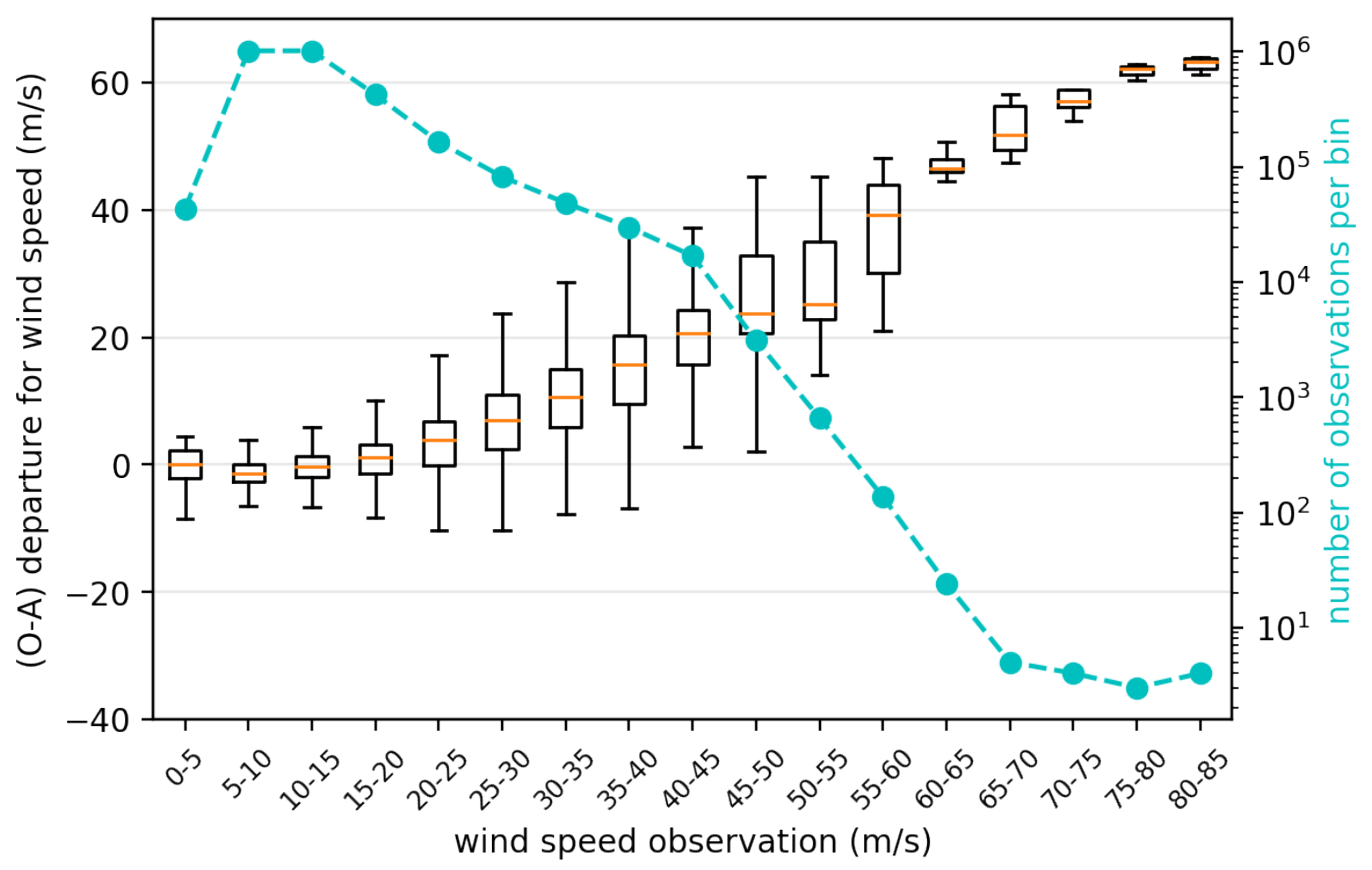
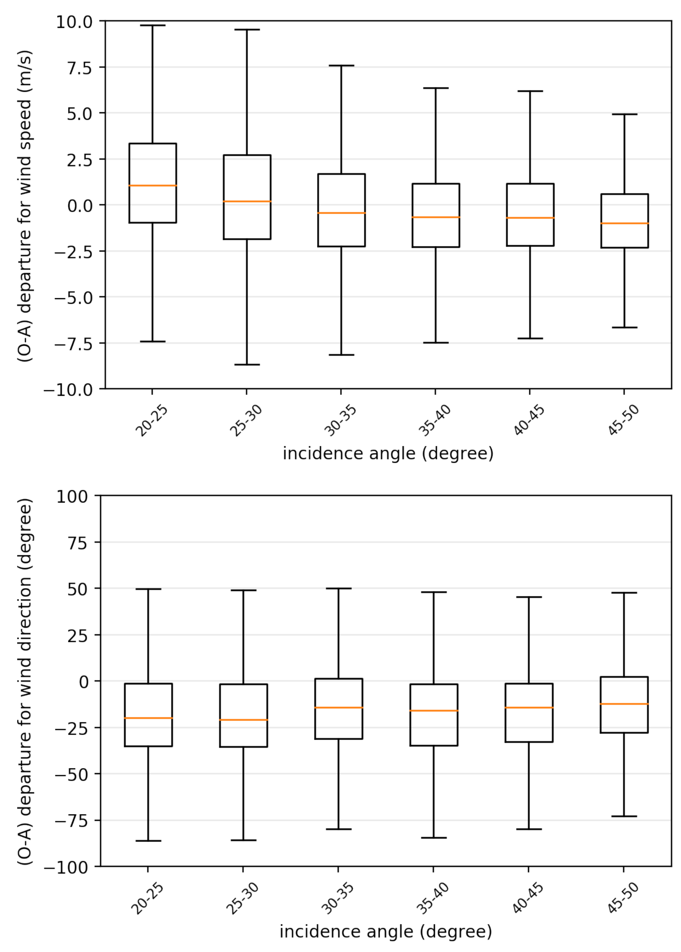
4.1. Assessment with AROME OI 3D-Var Analyses

Here, 3-km resolution wind speed and direction derived from SAR images are compared to neutral wind speed interpolated from AROME OI 3D-Var model analyses which are the nearest to the time acquisition of the SAR images. Thus, the time lag between a SAR observation and the model analysis used as reference is less than 30 min and should not be responsible for TC position error larger than 10 km, considering that most TCs have a velocity between 10 and 20 km·h${}^{-1}$. Figure 1 shows that in low wind speed range, observations and model are close to each other, but discrepancies grows as observation values become larger, over 25 m·s${}^{-1}$. Over this threshold, the gap between observations and model tends to dramatically increase for extreme high values. The relative contribution of analysis error and observation error to this gap is hard to estimate in extreme wind conditions due to a low number of data. Highest wind speed values are found in the TC eyewall. Model analysis error could be attributed to a misplacement of the TC eyewall position and/or a poor estimation of its diameter, or a misrepresentation of TC intensity.

For wind speed values below 25 m·s${}^{-1}$, observation departure to model analysis (O-A) bias is computed at −0.24 m·s${}^{-1}$ and standard deviation at 3.11 m·s${}^{-1}$. For wind speed values above 25 m·s${}^{-1}$, (O-A) bias is computed at 10.87 m·s${}^{-1}$ and standard deviation at 8.54 m·s${}^{-1}$. With the hypothesis that analysis wind speed is unbiased, the (O-A) bias is equivalent to an estimated observation bias.

For low values, for u and v components of wind speed, (O-A) follow a Gaussian distribution (Figure 2), which is necessary in theory for a correct data assimilation in the 3D-Var scheme. On the contrary, for high wind values, the u and v components of wind do not respect a Gaussian distribution (Figure 3) and are highly biased. One cause is probably that TC model location is displaced from the observations, which is known to represent a challenge for a correct assimilation in the high wind speed range [21].

The relationship between (O-A) and the incidence angle of the sensor is also investigated (Figure 4). (O-A) for wind speed is more important at low and high incidence angles with 1-m·s${}^{-1}$ positive bias for the 20–25° range and 1-m·s${}^{-1}$ negative bias for the 40–45° range. For wind direction, a negative bias between 15 and 20 degrees is observed for the whole range of incidence angle. The sign of the bias is consistent with previous studies from [13,14], indicating that HBL rolls tilted towards the center, while the extent is larger that the expected 10${}^{\circ }$. Some additional tests were conducted to assess the impact of the TC misplacement between these SAR observations and ECMWF model analyses. They have shown that the difference between the model wind direction and the HBL rolls orientation is reduced by 6${}^{\circ }$ if placing the SAR-observed TC eye at the modeled location. As for the wind speed, correcting for TC misplacement would increase the wind speed bias by 0.3 m·s${}^{-1}$, which would thus increase the agreement at high incidence angles.

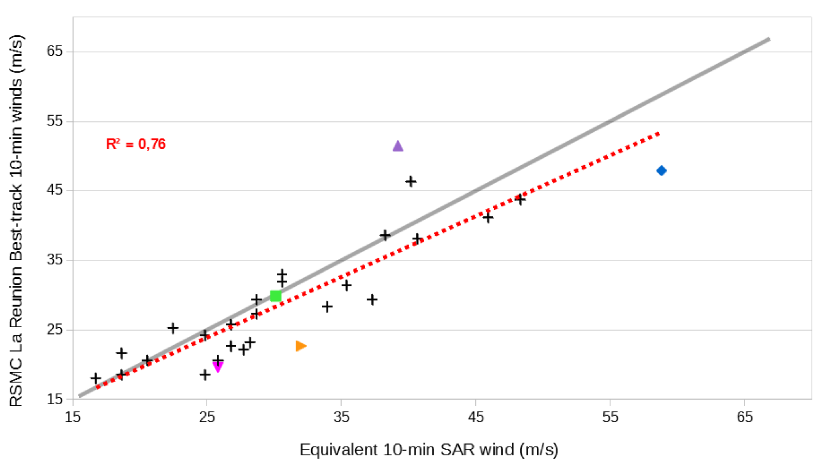
4.2. Assessment with Best Track Database

Tropical cyclone forecasters at RSMC La Reunion do not regularly benefit from in situ measurements within tropical cyclones as it is the case in the North Atlantic or, to a lesser extend, in the Northwest Pacific, when the systems approach inhabited lands. In the SWIO, the TC intensity is defined as the maximum wind averaged over 10 min within the clockwise circulation (Vmax) according to the operational Tropical Cyclone Plan [22]. This has been estimated since 1982 by applying the Dvorak technique [23,24] which uses the link between the cloud configuration of a system in infrared or visible imagery and the strength of winds at the surface. Since the late 1990s, forecasters have also been using information from microwave imagers/sounders and the objective guidance associated (ADT, AMSU, SATCON) along with scatterometers data such as the currently operational ASCAT and SCATSAT, to refine intensity estimation. On the other hand, it can also be recalled that part of the forecaster’s work consists in evaluating in real time structural parameters of a TC such as the radius of maximum winds (RMW) and wind radii for 28, 34, 48 and 64 kt (14.4, 17.5, 24.7, 32.9 m·s${}^{-1}$) winds, in order to assess its destructive potential (extension of destructive winds, storm surge forecast). In this context, the exploitation in near-real time of SAR wind data is expected to make it possible to estimate quantitatively and for the first time, the size and intensity of TC inner core thus significantly improving the quality of the warnings issued to the threatened populations.

In addition to acquisitions made in the framework of the ReNovRisk campaign, 30 complete acquisitions (RMW completely sampled) have been made for SWIO TCs between February 2017 and March 2020. During that period, the SAR data were compared to the BT data of maximum winds (thereafter BTMW) interpolated at the time of the swath. The SAR wind data resolution of 3 km are close to 1-min averaged winds based on inter-comparisons between SAR winds and winds estimated by the on-board Stepped Frequency Microwave Radiometer (SFMR) on reconnaissance aircraft [11]. On SAR acquisitions, the SAR maximum winds (SARMW thereafter) selected as a measure of TC intensity should be representative of the eyewall area where the strongest winds are found (not only the strongest 3-km wind pixel). In practice, diagnostics based on the average profile in a given quadrant (NE, SE, SW or NO) associated with the maximum mean wind have been used to determine SARMW, similar to what was done in [25]. Since the BTMW is equivalent to a 10 min mean wind, a coefficient of 0.93 is applied to the first estimate of SARMW following [26] for the case “at sea” exposure. Note that over the comparison period, BTMW was not established by taking into account SAR data.

Figure 5 shows overall a fairly good correlation between the two data sources. However, for wind speed higher than 25 m·s${}^{-1}$, BTMW data tend to be lower than SARMW. In the absence of in situ data, it is not possible to conclude which data are more accurate. However, this finding can be partly explained by the biases highlighted by [27] on the Dvorak method, which nevertheless remains a leading tool for the determination of BTMW. Although caution should be applied to this results as they may only be valid in the North Atlantic, winds estimated between 15–25 m·s${}^{-1}$ by the Dvorak technique could be stronger in reality (1 or 2 m·s${}^{-1}$ on average), which is reflected by SARMW between 25–30 m·s${}^{-1}$, being mostly associated with BTMW between 15–25 m·s${}^{-1}$.

The case of tropical storm FRANCISCO illustrates this point (Figure 6): on 14 February 2020 when this system approaches the east coast of Madagascar, BTMW is assessed at 23 m·s${}^{-1}$ and is mainly based on Dvorak analysis. The S1A pass shows a very compact core with an RMW at about 9 km and an average 34-kt wind radius of about 20–30 km. SARMW reaches 32 m·s${}^{-1}$ (+9 m·s${}^{-1}$ compared to BTMW). Here, confidence in the strong winds estimated by the SAR pass may be reinforced by the small size of the system as the Dvorak technique tends to underestimate the intensity of small systems [27].

In some cases, SAR swath appears noisy due to sub-swath issues at low incidence angles. Figure 7 is an example of such a case with TC CARLOS seen by S1A on 7 February 2017 at 01:52Z. In this case, SARMW is 6 m·s${}^{-1}$ higher than BTMW but, from the SAR image, can be mostly explained by sub-swath’s winds with the lowest incidence angle being consistently stronger than the neighbouring sub-swath’s winds. Such a report is consistent with results from the previous section (Figure 4) where low incidence angle is associated with positive bias.

Some SAR passes with very little sub-swath issues have sometimes shown much stronger winds than BTMW and also stronger winds than any available subjective or objective guidance. It was the case with TC IDAI seen by S1A on 11 March 2019 at 02:46Z with a SARMW—BTMW difference reaching +11 m·s${}^{-1}$, making it a notable outlier of Figure 5. On the other hand, we report one significant case where BTMW is significantly stronger than SARMW. BTMW for TC JOANINHA on 28 March 2019 at 00Z is at 51 m·s${}^{-1}$, based on Dvorak analysis and a clear cut eye pattern. This value appears 12 m·s${}^{-1}$ stronger than the SARMW from a RS-2 swath at 00:52Z (Figure 8). Strong discrepancies on these two cases of IDAI and JOANINHA remain not fully understood at this time, but it is likely that incidence angle issue and/or rain attenuation (Figures 7 and 8 in [11]) may have played a role.

Overall, SARMW and BTMW have been in fairly good agreement, which means that most of the time, SAR data and other referent tools for TC intensity analysis (Dvorak methods, objective guidance, scatterometric data, etc.) tell “the same story” about TC strength. Some cases demonstrate discrepancies that could be explained at least partly by known biases of the usual guidance and/or SAR sampling issues. Whether or not forecasters should favor SAR winds when they are significantly higher/lower than the usual guidance, remains an open question at this time. However, with further development on SAR data post-processing and ongoing work on the validation of their quality, they may become an essential source of information for refining intensity, position and structural parameters of TC monitored over the SWIO.

5. Assimilation of SAR Data with AROME 3D-Var

Two case studies are presented hereafter to assess the potential impact of SAR assimilation with AROME OI 3D-Var. The SAR image captured on 7 February 2019 02:09Z provides a complete description of surface wind structure of GELENA, while the SAR image captured on 11 March 2019 02:46Z details the inner structure of TC IDAI. In both cases, at acquisition time, the systems are in intensification stage, underwent severe tropical storm or tropical cyclone status for a few hours, far from landfall, with high potential for intensification.

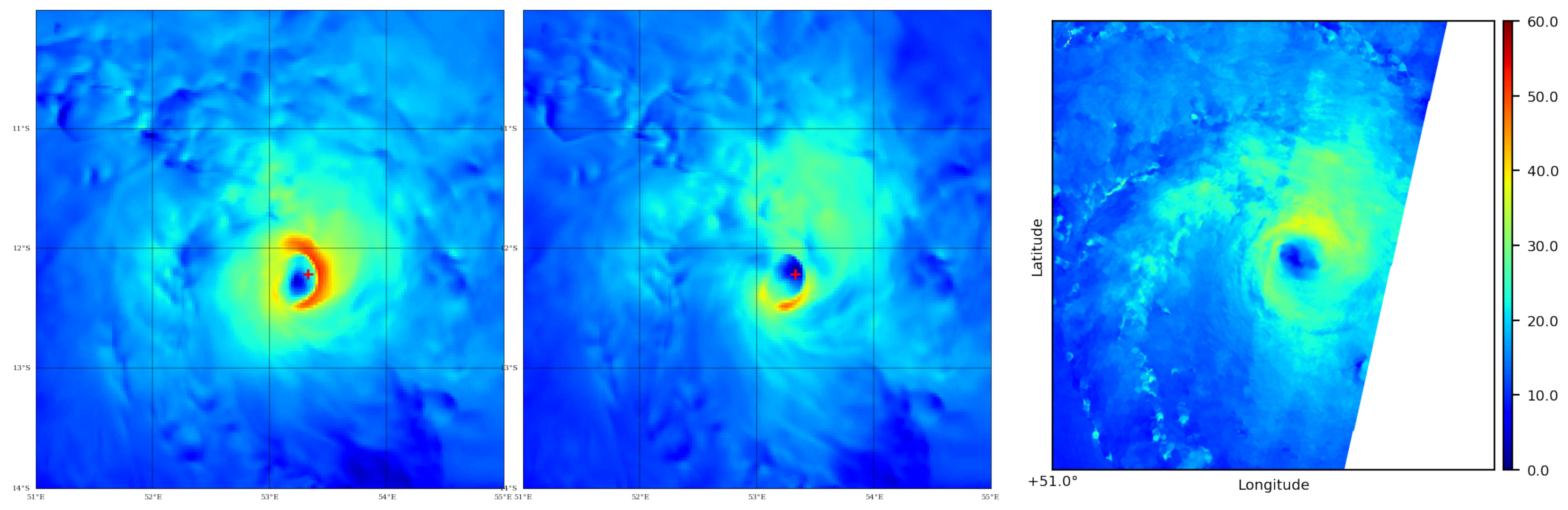
5.1. Case of TC GELENA

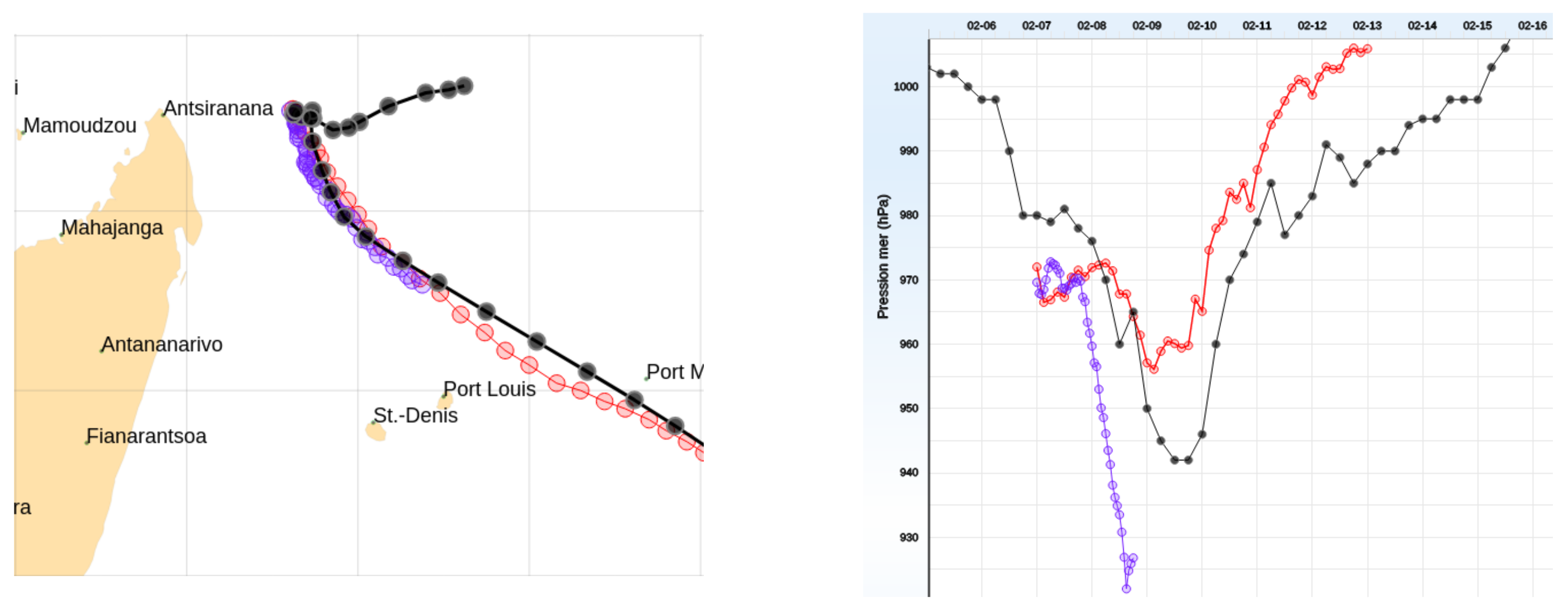
5.1.1. Description of Cyclone GELENA

GELENA formed within an active monsoon trough taking place in early February 2019 over the SWIO from a low pressure area located less than 1000 km east of Diego–Suarez (northern tip of Madagascar). Its development rate became rapid from the night of 5 to 6 February, where the system became a tropical storm late at night and then a severe tropical storm, close to tropical cyclone status, late on 6 February. On early 7 February, it gradually accelerated southward then south-eastwards ahead of a deep layer mid-latitude trough. GELENA, which weakened slightly on 7 February due to slow motion-induced sea surface temperature cooling, resumed an intensification trend and became a tropical cyclone on the morning of 8 February and then an intense tropical cyclone (equivalent CAT3 on the US Saffir–Simpson scale) 24 h later. GELENA reached its maximum intensity in the early afternoon of 9 February, with estimated maximum winds over 10 min at 57 m·s${}^{-1}$ (equivalent CAT4 on the US Saffir–Simpson scale) and a minimum sea level pressure (MSLP) of 938 hPa, before weakening due to vertical shear. At the end of the night, GELENA came 60 km closer to Rodrigues Island (42,000 inhab.), still being an intense cyclone. The island escaped the eyewall but experienced violent wind gusts recorded at 46 m·s${}^{-1}$ at Pointe-Canon. During the following days, on a south-eastwards then east-south-eastwards track, GELENA slowly filled up and dissipated late on 16 February to the East of 90° E in the subtropical domain.

Operational models used at RSMC, IFS and AROME-OI, represented for most of analyses of 7 February a TC more intense than estimated by BT. In Figure 9, from 00:00Z analyses, MSLP forecasted by both models is lower than in BT by 6–13 hPa until 7 February 18:00Z. After, AROME-OI forecasts an over-intensification of the TC, while IFS forecasts show a more realistic pattern for intensification from 8 February 00:00Z to 9 February 00:00Z. On a longer lead time, IFS forecasts an early weakening of TC starting from 9 February 00:00Z. It can be noted that forecasts available later hardly corrected the mistimed TC weakening. SARMW from the image captured on 7 February 2019 02:09Z matches the BTMW very well (Figure 5).

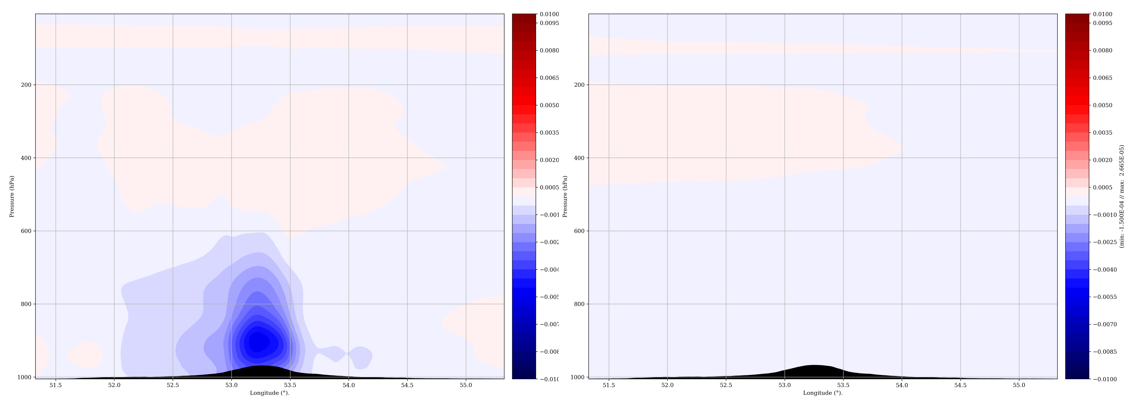
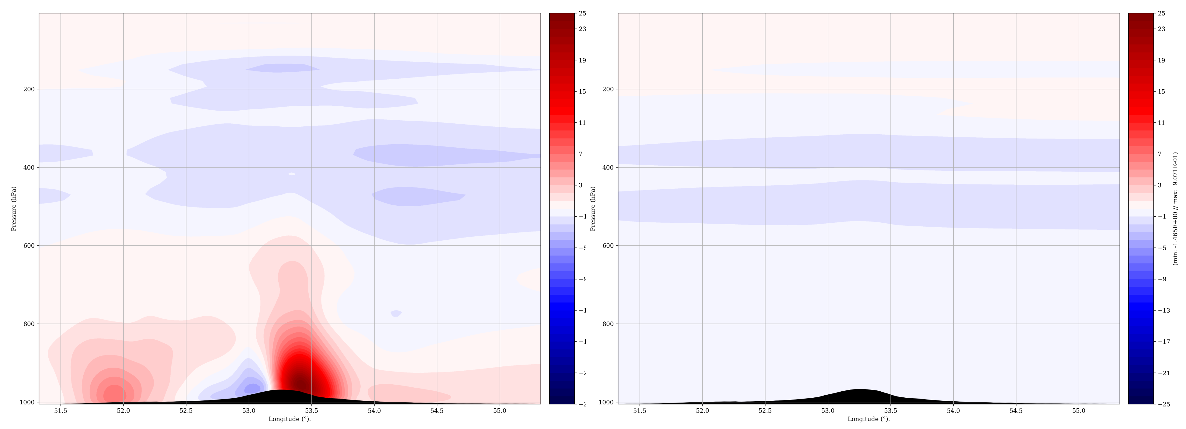
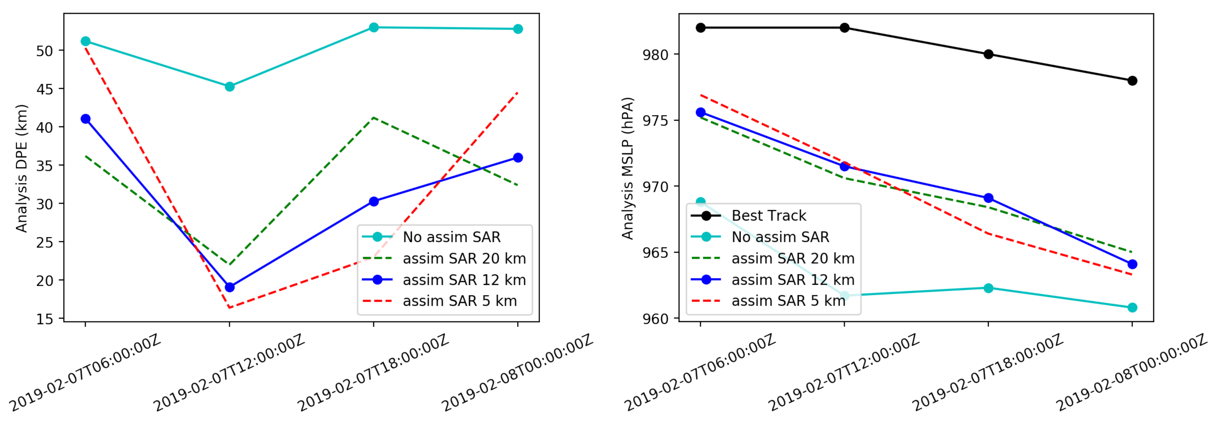
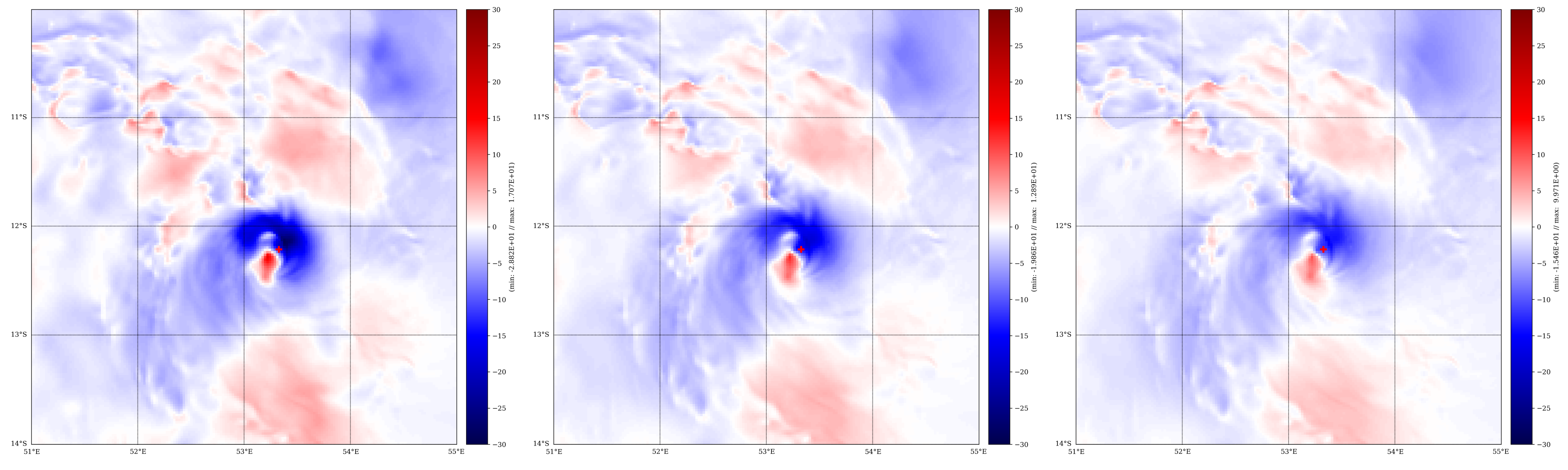
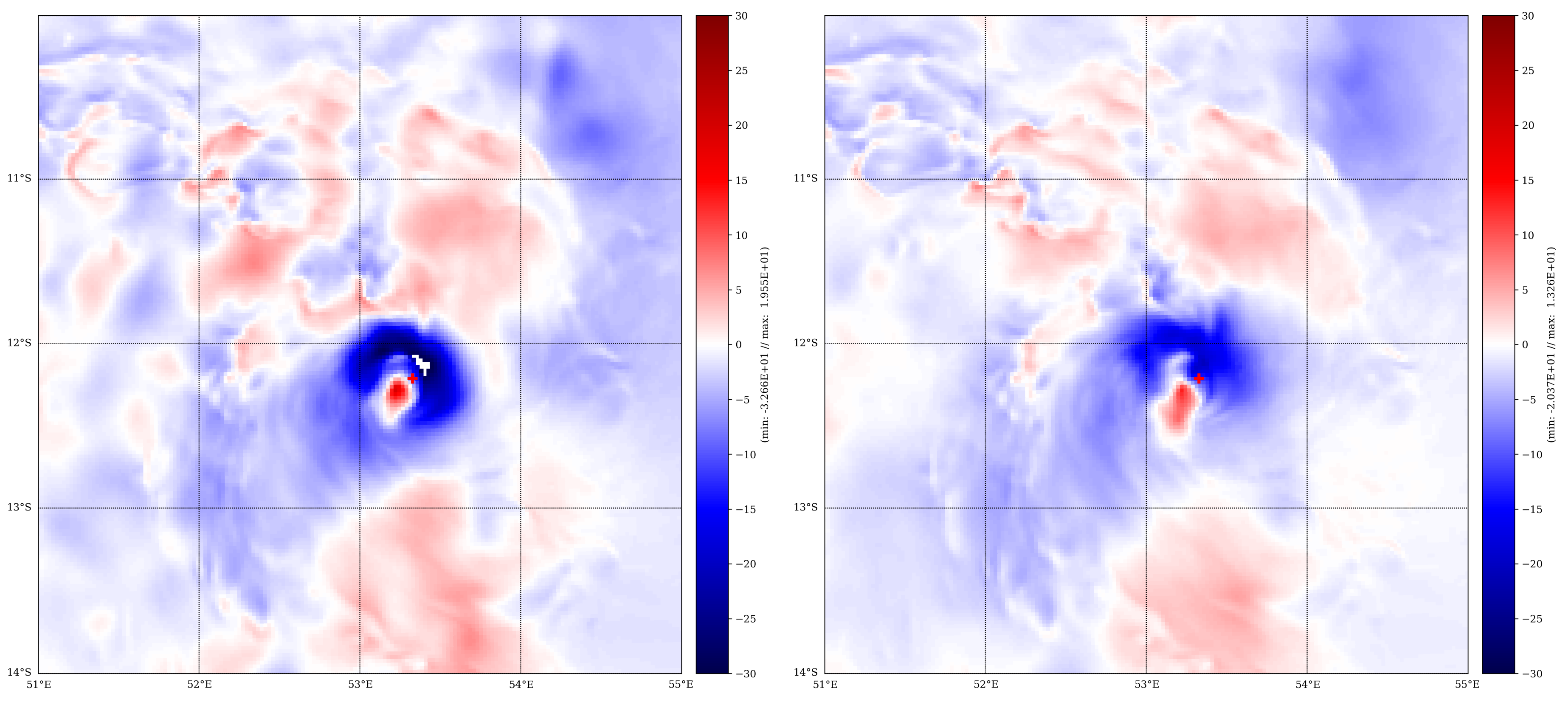
5.1.2. Impact on Analyses

In this section, the result of the SAR_12km_2ms experiment for which SAR data are assimilated on 7 February 2019 02:00Z is compared to the reference experiment NO_SAR. In SAR_12km_2ms, the SAR observation error is set to 2 m·s${}^{-1}$ and thinning to 12 km. As shown by Figure 10, the analysis for surface wind speed for 7 February 2019 02:00Z shows important updates to its background. On the southern part of the TC eye, wind speed increment are larger than 25 m·s${}^{-1}$. As a consequence of the SAR data assimilation, surface winds become significantly weaker in a large area covered by the SAR image, especially in the inner vortex and the eyewall.

In the eyewall of the background, (O-B) is many times the standard observation error, so observations located in that area may not explain the analysis increment. However, in areas outside and inside of the background eyewall, (O-B) is much smaller. So, observations in there are considered confident observation and have more impact on the analysis increment. In the 3D-Var assimilation process, a SAR observation will bring analysis increment at its location but also on neighbor grid points. The spatial extension of its influence will depend on the proximity of other observations and the confidence given to them. So, low wind speed observations located immediately outside and inside the background eyewall will contribute to reduce its strength.

The outer vortex wind structure in the analysis converges toward the one captured by SAR observations. The TC center is displaced north-eastward. SAR data assimilation has thus a positive impact on TC center position, as Figure 10 shows that the TC center in the background is south-westward of the position interpolated from positions given by the BT on 7 February 2019 00:00Z and 06:00Z.

SAR data assimilation is also responsible for analysis increments in wind, temperature and humidity at upper levels in the eye and eyewall area. As mentioned in Section 3, the 3D-Var scheme propagates analysis increment in wind to other control variables such as temperature and specific humidity. Figure 11, Figure 12, Figure 13 and Figure 14 show analysis increments for vertical zonal section centered on the TC eye for different variables. For temperature (Figure 11), besides the strong negative analysis increment from surface to 900 hPa, a second negative analysis increment can be spotted, centered at 600 hPa over a vertical thickness of 300 hPa. For specific humidity (Figure 12), a negative analysis increment can be noticed over a vertical thickness of 250 hPa with a maximum around 900 hPa. The global loss of temperature and humidity can be interpreted as a removal of heat content in the TC warm core, which is coherent with an analysed TC becoming weaker. For zonal and meridian wind (Figure 13 and Figure 14), although the maximum analysis increment is at the surface, analysis increment develops as high as 600 hPa for meridian wind and 400 hPa for zonal wind. The reference experiment NO_SAR shows no such analysis increments, ensuring that dynamic and thermodynamic vortex structure modification is due to SAR data assimilation.

The information brought by SAR observations has an impact on, but is not limited to, the analysis at the time of assimilation. Through the assimilation cycle, because each analysis is built upon the forecast of the previous analysis, a TC modification in intensity, position or structure induced by the assimilation a SAR image can propagate for several hours and affect the subsequent analyses.

The strength of the TC and its evolution can also be followed with integrated kinetic energy (IKE), defined for example as:

$$IKE=\int \frac{1}{2}\rho U^{2}dV$$

(1)

where here, U is the AROME OI 3D-Var surface wind speed on a grid point, $dV$ is the elementary volume unit, i.e., the surface model represented by a grid point (2.5 × 2.5 km) multiplied by a thickness of 1 m and $\rho$ is the air density fixed at 1.2 kg/m${}^3$. The contribution of turbulent wind fluctuation is not taken into account in the calculation of IKE.

Adapted from [28], this definition of IKE, on the contrary to Vmax, gives a diagnostic on both the horizontal spatial extent and the strength of the wind. Hence, it is a better indicator for the wind destructive potential of TC, also easily accessible from gridded surface wind fields. In a sense, it synthesizes information from Vmax and other TC structure parameters such as RMW, and 34- or 64-kt wind radii. As SAR data assimilation has an impact on the analysis on a large area, its effect on IKE is to be also more noticeable than on Vmax. We follow 2 different IKEs: the one contained in area of surface wind speed around TC center above 34 kt (IKE34) and another above 64 kt (IKE64). In the SWIO, 34 kt and 64 kt are the thresholds on Vmax for classifying a system as a tropical storm and a tropical cyclone, respectively.

The impact of SAR assimilation on the analyses is quantified by comparing analyses from NO_SAR and SAR_12km_2ms. Figure 15 shows that wind analysis increments seen in SAR_12km_2ms reduces IKE34 from 14.5 TJ to approximately 11 TJ, equivalent to a reduction of 20–25 per cent on 7 February 2019 02:00Z. The subsequent analyses suggest that this IKE34 reduction is still persistent, at least until 7 February 2019 09:00Z, 7 h later. This IKE34 reduction is comparable in duration to the one obtained by the assimilation of scatterometer data such as ASCAT when the TC eye is sampled (not shown). It must be noted that IKE34 derived from observed SAR image is estimated at 16 TJ. One has to consider this value cautiously, because a large part of the vortex can be found in the subswath of low angle, which is known to have positive biases, so IKE34 may be overestimated by S1 SAR in this case. However, one may expect IKE34 for SAR_12km_2ms to be closer to IKE34 from observed SAR than IKE34 for NO_SAR as the analysis in SAR_12km_2ms reproduces partly the observed outer vortex wind structure as mentioned earlier. It does not happen, firstly because of the misalignment of wind structures such as spiral bands between background and SAR image. In that case, the 3D-Var data assimilation process, which combines background and observation wind fields, tends to produce a smoothened wind field with smaller wind gradients and diminished maximum wind speed values, resulting in an IKE34 diagnostic decrease. Secondly, IKE34 encompasses IKE64, which dramatically decreases, as explained hereafter.

The impact of SAR data on IKE64 is even more consequent, with IKE64 dropping from 3 TJ to 0.5 TJ on 7 February 2019 02:00Z, equivalent to a reduction of roughly 80 per cent. The IKE reduction persists at least until 7 February 2019 23:00Z, with an average 2-TJ departure between NO_SAR and SAR_12km_2ms. The removal of most winds above 64 kts makes GELENA model representation in SAR_12km_2ms more consistent with BT, as GELENA is classified as a severe tropical storm on 7 February 2019, before gradually strengthening to become a TC on early 8 February 2019.

Hence, SAR data, through assimilation, have the ability to modify the surface wind field of a TC in a significant manner. In this case, it can drastically reduce the strongest winds in the inner vortex.

Comparisons with BT show that analyses from NO_SAR experiment overestimate the strength of GELENA (at least in terms of Vmax and MSLP) and would classify the system as a TC instead of a severe storm on the 7 February 2019, so corrections made through SAR can be considered useful improvements for operational guidance.

SAR measurements were demonstrated to have unique high-resolution capabilities, capturing the inner- and outer-core radial structure of the TC vortex [29]. Analysis increment at 02:00Z and evolution of IKE 34 and IKE64 in the subsequent analyses show that this additional inner- and outer-core radial structure of TC vortex are taken into account during assimilation and propagate well for subsequent hours.

The removal of global energy diagnosed through IKE34 and IKE64 in SAR assimilating experiments also impacts on MSLP, which is assessed by BT every 6 h. MSLP in SAR_12km_2ms is 7–10 hPa closer to BT than in NO_SAR for analyses on 7 February 2019 06:00Z, 12:00Z, 18:00Z and on 8 February 2019 00:00Z.

Direct positioning error (DPE) is the position error of the TC center in an experiment compared to BT (available for 00:00, 06:00, 12:00, 18:00Z). here, the TC Center in the model is tracked by searching the MSLP.

Figure 16 shows that the position of the TC center is also improved by assimilating SAR. When comparing NO_SAR and SAR_12km_2ms on 7 February 2019, DPE is reduced by 10 to 26 km for analyses on 7 February 2019 06:00Z, 12:00Z, 18:00Z and on 8 February 2019 00:00Z.

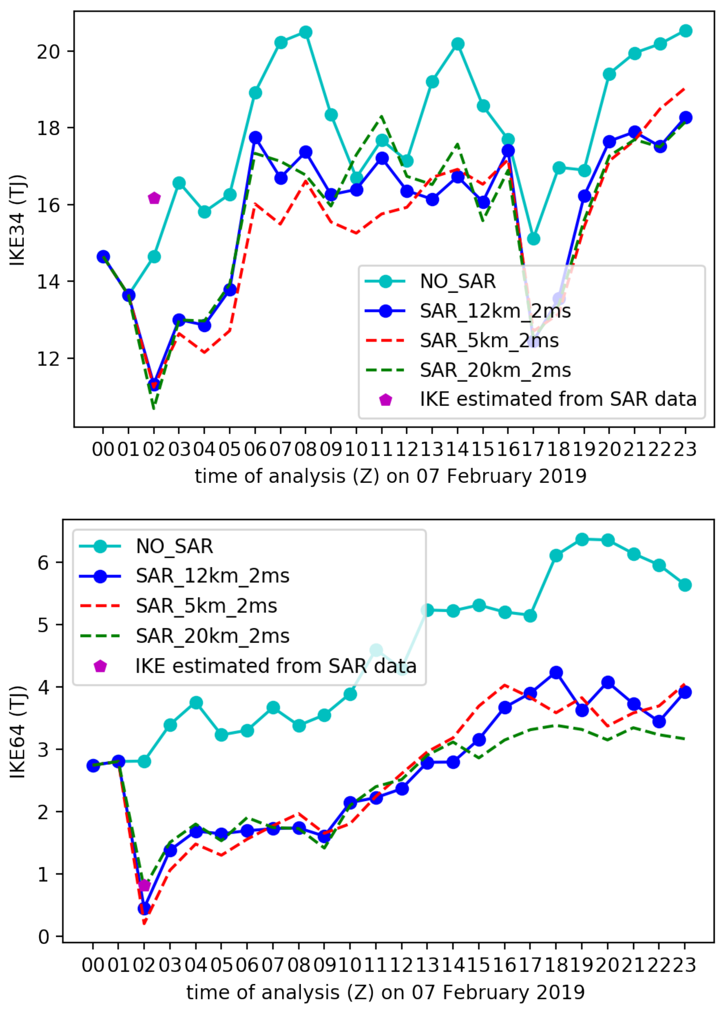
5.1.3. Impact on Forecasts

General improvement of the few analyses following SAR data assimilation on 7 February 2019 02:00Z was presented in the previous subsection. It is expected that at least short-term forecasts are also improved. A 42-h forecast starts from the 7 February 2019 06:00Z analysis in experiments NO_SAR and SAR_12km_2ms. IKE34 and IKE64 forecasts are presented in Figure 17. On IKE34, SAR have no impact further than 6-h lead time. On the contrary, regarding IKE64, SAR impact is still significant at 12-h lead time and still persists, to a lesser extent, until 18-h lead time. Therefore SAR data shows the ability to modify the surface wind field for strong wind values, not only for analyses, but also for 12 h-forecasts.

5.1.4. Sensitivity Tests

In addition to NO_SAR and SAR_12km_2ms, 4 other experiments are run as sensitivity tests. Assimilation for an observation type can be optimized through 2 parameters: observation error and thinning. In a first series of sensitivity test, data thinning is set to 12 km, but the observation error is set to 4 m·s${}^{-1}$ for SAR_12km_4ms and to 6 m·s${}^{-1}$ for SAR_12km_6ms. Increasing the observation error lowers the observation weight, diminishing the impact of SAR observations in the analysis of 7 February 02:00Z, as shown in Figure 18. The TC weakening in the analyses of SAR_12km_4ms and SAR_12km_6ms is lessened compared to the analysis of SAR_12km_2ms. This difference is also diagnosed by MSLP of the subsequent analyses of 7 February. MSLP in analyses of SAR_12km_2ms is 1-2 hPa closer to BT than in analyses of SAR_12km_4ms and SAR_12km_6ms (not shown).

In a second series of tests, the observation error is set to 2 m·s${}^{-1}$. Thinning is set to 5 km for SAR_5km_2ms experiment and to 20 km for SAR_20km_2ms. Figure 19 shows the impact of data thinning. Increasing the density of assimilated observation augments the analysis increment, while assimilating less observations has the inverse effect.

Analysis increments from all experiments show a similar dipole with reinforcement (reduction) of wind speed southwestward (northwestward) of TC center, meaning that the assimilation process displaced the TC center northeastward, as mentioned earlier. The analysis increment is also negative in the eyewall region, notably in the upper half circle, meaning that energy is removed in that region. In Figure 16, sensitivity to thinning for the subsequent analyses are presented. SAR_20km_2ms and SAR_5km_2ms show only a 2-hPa MSLP difference from SAR_12km_2ms and all experiments show improvements in DPE compared to NO_SAR. However, SAR_5km_2ms seems more unstable: on 7 February 06:00Z, DPE is no better than for NO_SAR, and in terms of MSLP, it is closer to BT on 7 February 06:00Z, then closer to NO_SAR on 7 February 18:00Z and 8 February 00:00Z. Assimilating SAR observation at such horizontal high resolution may become suboptimal due to potential correlation between observation errors [30], but experiments run on more cases are needed to confirm this hypothesis. As for forecasts, the reduction of IKE64 in forecast from SAR_20km_2ms and SAR_5km_2ms is similar to the one found in SAR_12km_2ms until 12-h lead time and even stronger at 18-h lead time (Figure 17).

The sensitivity tests confirm that results found on the impact of SAR assimilation on analysis and forecast are robust to different settings. SAR data assimilation with optimal settings should show the most positive impact compared to BT, not only for the analysis at assimilation time, but also for the subsequent analyses of the day.

5.2. Case of TC IDAI

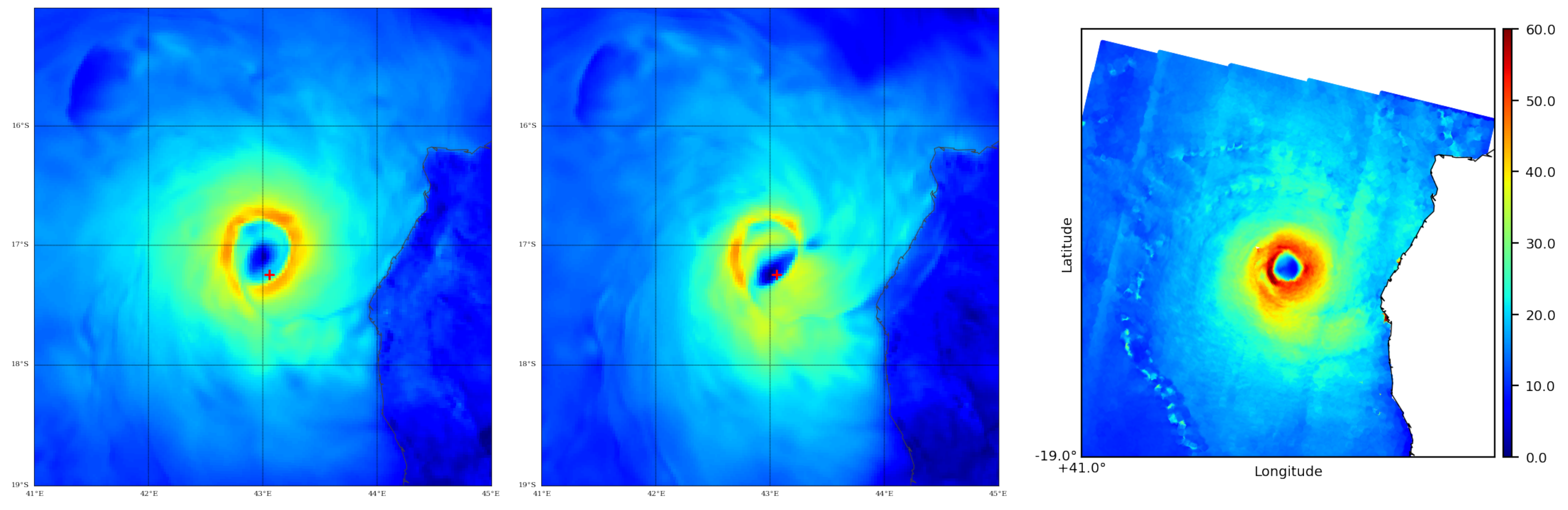
5.2.1. Description of Cyclone IDAI

TC IDAI started to develop on 4 March 2019 close to the coastline of the province of Zambézia (Mozambique) as a tropical depression, and quickly intensified to a tropical storm before made a first landfall on the same day. A remnant of low pressure persisted over land with associated thunderstorms and heavy rainfall affected several provinces of Malawi and Mozambique. On 9 March, the remnant low pressure moved back over waters in the Mozambique Channel. Overseas, it intensified rapidly, maturing into a tropical cyclone late on 10 March and into an intense tropical cyclone with estimated maximum 10-min winds at 51 m·s${}^{-1}$ and MSLP at 942 hPa on 11 March (equivalent CAT4 on the Saffir–Simpson scale). As it was located off the western coasts of Madagascar, IDAI reversed its track early on 11 March towards the Mozambican coastline. IDAI weakened as an eyewall replacement cycle occurred, but intensified again on 13 March, with a life maximum intensity reached at 18:00Z associated with estimated maximum 10-min winds of 54 m·s${}^{-1}$ and 940 hPa at the center (again CAT4). Some weakening took place before landfall, which eventually occurred on the evening of 14 March, around 22UTC, in the northern vicinity of Beira. Maximum 10-min wind was estimated at 46 m·s${}^{-1}$ and MSLP at 955 hPa, by the time of landfall. No surface observation was reported from Beira. It rapidly weakened as it moved inland.

Forecasts from operational models used at RSMC, IFS and AROME-OI, starting from 11 March 2019 00:00Z, underestimated TC intensity until 11 March 2019 12:00Z. After, none of them manage to simulate the eye replacement cycle and associated weakening. Instead, after slowing down for a few hours, IDAI intensified again rapidly in both models. The overintensification is larger in AROME-OI forecasts than in IFS forecasts (Figure 20). SARMW derived from the image captured on 11 March 2019 2:43Z is significantly stronger than BTMW (Figure 5).

5.2.2. Impact on Analyses

SAR data are assimilated on 11 March 2019 03:00Z in the SAR_12km_2ms experiment. In the 3D-Var background, the TC is well organised, with strong winds in the eyewall (above 30 m·s${}^{-1}$). However, the TC eye diameter of the background is approximately twice larger than in the SAR image (Figure 21) and SAR wind speed is much more intense in the inner vortex. Comparisons between the analysis and the background from SAR_12km_2ms show that the TC center is displaced southward by the SAR data assimilation. The new position of the TC better matches the position estimated by BT. Moreover, the winds are reinforced in the southern part of the outer vortex. Hence, as for GELENA, the outer vortex wind structure in the analysis is closer to the SAR observations than in the background. However, the inner vortex wind structure in the analysis is very different from the one given by the SAR image. In particular, the 3D-Var assimilation process fails to remove completely the initial eyewall, which was misplaced in the background, and it is not able either to construct a new thick eyewall as seen in the SAR image. In this case, the 3D-Var is not able to conserve the structure of the original strong vortex in the relocation process. The resulting system in the analysis is unbalanced, and it even shows a double eyewall northwestern of the TC center.

The destructuration of the TC in the analysis, due to the misalignement of wind structures between background in SAR_12km_2ms and SAR image, is diagnosed by IKE64/IKE34 (Figure 22), which shows that the intensity of the TC is reduced by the SAR assimilation despite the very large value of the observed winds. IKE64 (IKE34) is reduced by 40–50 (20–25) percent in SAR_12km_2ms compared to NO_SAR on 11 March 03:00Z. On the contrary, IKE34 and IKE64 estimated from SAR data are 3 to 6 TJ stronger than in NO_SAR.

This IKE reduction due to the vortex destructuration propagates through the subsequent analyses for 9–10 h for IKE34 and 15–16 h for IKE64. It is also diagnosed on MSLP, where SAR_12km_2ms analyses show higher MSLP than NO_SAR analyses (Figure 23).

However, the TC intensification rate (seen, for example, with the slopes of the curve of the MSLP minima on Figure 23) remains very high even when the structure of the TC is damaged by the assimilation of SAR data at 03:00Z. It shows that in this case, the intensification of the TC is not only controlled by the state of the cyclone in the initial conditions, but it also strongly depends on the larger scale and the ability of the model to simulate the physics of the TC intensification.

In terms of DPE, the improvement of the TC position shown in the 11 March 2019 03:00Z analysis is not seen in the subsequent analyses (Figure 23). However, the DPE remains under 45 km which, compared to BT uncertainty on TC position estimated around 40 km, show that both SAR_12km_2ms and NO_SAR experiments perform quite well in this case to determine TC center position.

This experiment on IDAI highlights that correcting the position of an intense TC already present in the background while preserving cyclonic structure with realistic features is challenging for data assimilation in high resolution numerical models, as discussed in [31]. This is particularly difficult for a 3D-Var system which does not have a linear tangent (and adjoint) of the model to physically constrain the increments.

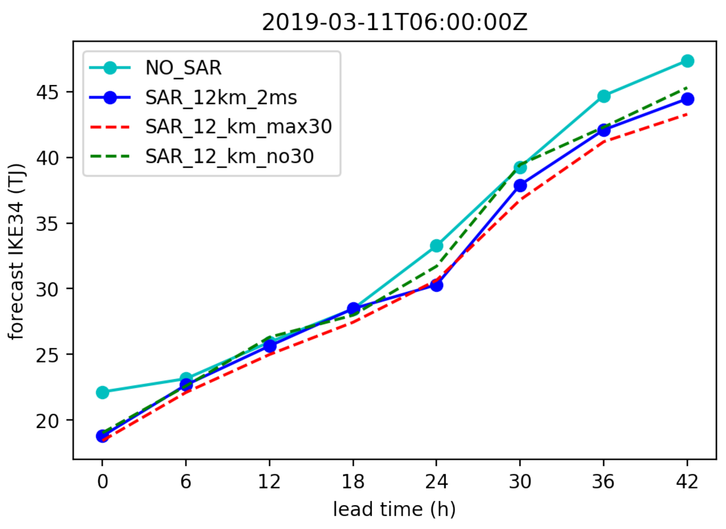
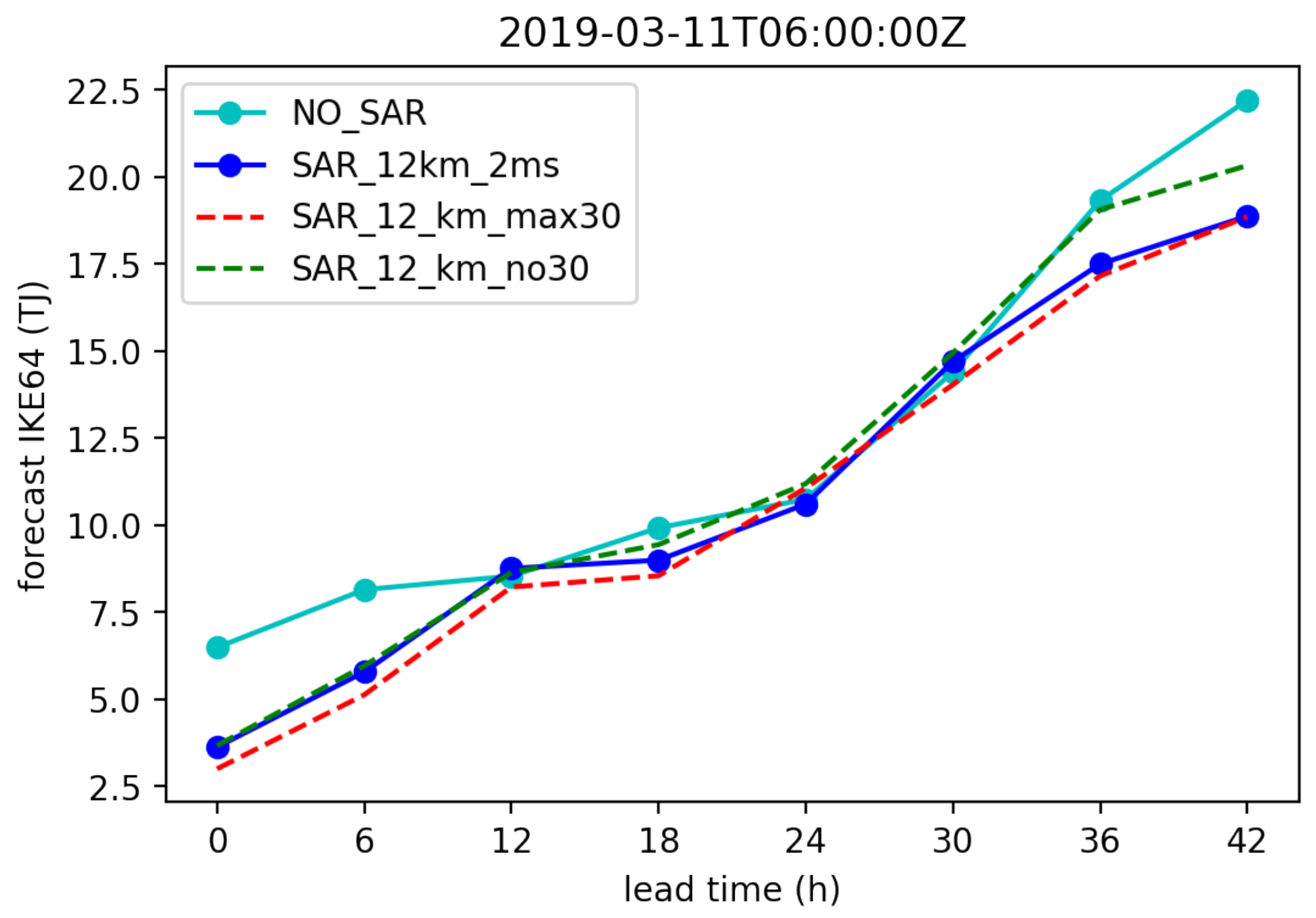
5.2.3. Impact on Forecasts

Moreover, 42-h lead time forecast starts from 11 March 2019 06:00Z from experiments NO_SAR and SAR_12km_2ms. IKE34 and IKE64 forecasts are presented in Figure 24. The SAR data assimilation has no impact on IKE34 further than 6-h lead time, while a difference between NO_SAR and SAR_12km_2ms is still seen until 12-h lead time.

5.2.4. Sensitivity Tests

As mentioned earlier, SAR gives access to observations in high wind speed range like no other remote sensor. A meaningful part of observations in the SAR image captured on 11 March 2:43Z contains high wind speed values, especially in the eyewall. Sensitivity tests are conducted to assess the impact of assimilating high speed observations, not accessible through scatterometers such as ASCAT.

In addition to the experiment SAR_12km_2ms, two similar experiments are run with modifications of SAR data which are assimilated. In SAR_12km_2ms_no30, only SAR data with wind speed below 30 m·s${}^{-1}$ are assimilated. In SAR_12km_max_30, SAR data with wind speed above 30 m·s${}^{-1}$ are set to 30 m·s${}^{-1}$. Figure 25 shows the SAR data assimilated within 51° E–55° E, 10° S–14° S in the 3 experiments.

As in SAR_12km_2ms, the TC center in both sensitivity experiments is displaced southeastward from background to analysis, as diagnosed by the dipole in the wind speed analysis increment, with positive analysis increment centered on the TC center in the background and a negative increment around the TC center in the SAR image (Figure 26). It is likely that high-speed SAR observations play a minor part in displacing TC eye. In SAR_12km_2ms_no30, the low wind speed SAR data within TC eye result in larger negative analysis increment. It is probable that these data are the ones which are responsible for TC eye relocation.

In both sensitivity experiments, the TC eye displacement in the analysis is destructuring the TC vortex as in SAR_12km_2ms and the TC intensity weakens after the assimilation of the SAR data, despite the very strong wind observed in the SAR image. A spin-up period of 2–3 h is necessary for the model to rebuilt a structured vortex that intensify again in the subsequent analyses (and forecasts), as shown in the evolution of IKE34 and IKE64 in Figure 22. Thus, higher speed SAR observations are not directly responsible for the creation of an unbalanced vortex in the analysis.

High-speed SAR observations have, nevertheless, a positive impact on TC intensity. In both sensitivity experiments, where they are limited in SAR_12km_max_30 and even removed in SAR_12km_no_30, the positive analysis increment is weaker than in SAR_12km_2ms and the negative analysis increment is reinforced. It highlights that, despite large (O-B), high-speed SAR observations are still assimilated, play a role in the magnitude of the positive analysis increment and also limit the negative analysis increment. This impact on TC intensity propagates through the analyses of 11 March 2019, as shown in Figure 23 through the MSLP diagnostic. For analyses from 11 March 2019 06:00Z, 12:00Z and 18:00Z, we can see that MSLP is higher by 2–3 hPa in both SAR_12km_max30 and SAR_12km_no30 than in SAR_12km_2ms. However, the impact remains relatively small compared to a gap with NO_SAR or BT MSLP values. The sensitivity tests have little impact as well on IKE forecast from 11 March 2019 06:00Z analysis (Figure 24, confirming that in this case, perturbations of the initial vortex do not affect the TC intensification rate.

6. Discussion and Conclusions

C-band SAR show the potential to measure extreme wind speeds that are not accessible by other means in the SWIO. Although promising, their use as a complementary source of information for refining intensity, position and structural parameters of TC monitored over the SWIO is still subject to further validation. In particular, they show biases at low (20–25°) or high (40–45°) angles of incidence, and differences in maximum winds between SAR and BT can be large and only partly explained in the absence of in situ data.

SAR images also demonstrate great potential for capturing a well-defined TC eye, and the two case studies show that their assimilation corrects the TC eye position in the analysis, as long as low wind speed observations are still located in the TC eye of the background. The outer vortex wind structure is also drawn closer to the observations in both case studies. As for the inner vortex structure, the assimilation of SAR data is capable of reducing the TC intensity in the analysis when the wind speeds in the eyewall are overestimated in the background as seen in GELENA case. Analysis increments are not restricted to surface wind fields, but are also visible in the upper layers of the troposphere up to 400 hPa in temperature, humidity and wind. In this case, the 3D-Var manages to reproduce a well balanced vortex in the analysis. This kinetic energy reduction propagates to subsequent analyses through the assimilation cycle and persists approximately for 12 h. It also has a positive impact on the TC forecasts derived from 06:00Z analysis and 12:00Z analysis.

Intensifying the underestimated TC IDAI with the 3D-Var assimilation of SAR data was found to be more challenging. In this second case, the SAR data assimilation fails to preserve the structure of the original strong vortex in the relocation process. The sensitivity tests show that the impact of high wind speed SAR data (above 30 m·s${}^{-1}$) is not directly responsible for the lack of skill of the assimilation of the SAR data in this case. In a case where a very intense TC is misplaced, the departure to background is very large, as diagnosed also in [6], for example, and the 3D-Var suffers from a double penalty as very large increments are needed to remove the misplaced cyclone in the background and then large increments are needed to reintroduce an intense cyclone at the right location in the analysis.

In our two case studies, the modification of initial conditions through 3D-Var assimilation had little influence on the intensification rate of the TCs in the forecasts. It shows that other drivers than the initial conditions play a role in the TC intensification in the model, such as the state of environment of the TC, the representation of the interaction with the ocean and of the internal physical processes in the TC. Improving the representation of these others aspects in the model would help produce better forecasts, which in turn, would lead to better assimilation by providing background closer to observations, notably in the eyewall.

Nonetheless, ref. [32] estimates the errors which are arising from the mischaracterization of the initial intensity of the tropical cyclone dominate the intensity errors for the first 2–4 days, especially when the initial intensity is small. SAR can play a pivotal role to depict a more realistic TC vortex in initial conditions. To do so, it is important on the one hand, to improve SAR wind product quality to alleviate issues relative to noise, sub-swath gap or heavy rainfall area and on the other hand, to transpose as accurately as possible the information they bring on TC parameters into the analysis. Methods combining variational data assimilation with vortex bogussing have been explored to improve intensity and track forecast [33,34] and could help make a better use of SAR observations in TC initialization. The development of operational SAR products available in near real time would foster more comprehensive statistical studies on the impact of assimilating SAR data on NWP models. Associated with the parallel improvement of data assimilation schemes, their contribution in high resolution NWP models may not be limited to more realistic depiction of TC but also extended to better initialization of polar low, medicane or meso-scale structures such as squall lines.

References

1. Mouche, A.A.; Chapron, B.; Zhang, B.; Husson, R. Combined Co- and Cross-Polarized SAR Measurements Under Extreme Wind Conditions. IEEE Trans. Geosci. Remote Sens. 2017, 55, 6746–6755. [Google Scholar] [CrossRef]
2. Bentamy, A.; Croize-Fillon, D.; Perigaud, C. Characterization of ASCAT measurements based on buoy and QuikSCAT wind vector observations. Ocean Sci. 2008, 4, 265–274. [Google Scholar] [CrossRef] [Green Version]
3. Bousquet, O.; Barruol, G.; Cordier, E.; Barthe, C.; Bielli, S.; Calmer, R.; Rindraharisaona, E.; Roberts, G.; Tulet, P.; Amelie, V.; et al. Impact of Tropical Cyclones on Inhabited Areas of the SWIO Basin at Present and Future Horizons. Part 1: Overview and Observing Component of the Research Project RENOVRISK-CYCLONE. Atmosphere 2021, 5, 544. [Google Scholar] [CrossRef]
4. Barthe, C.; Bousquet, O.; Bielli, S.; Tulet, P.; Pianezze, J.; Claeys, M.; Tsai, C.-L.; Thompson, C.; Bonnardot, F.; Chauvin, F.; et al. Impact of tropical cyclones on inhabited areas of the SWIO basin at present and future horizons. Part 2: Modelling component of the research program RENOVRISK-CYCLONE. Atmosphere 2021. submitted. [Google Scholar]
5. Tulet, P.; Aunay, B.; Barruol, G.; Barthe, C.; Belon, R.; Bielli, S.; Bonnardot, F.; Bousquet, O.; Cammas, J.P.; Cattiaux, J.; et al. ReNovRisk: A multidisciplinary programme to study the cyclonic risks in the South-West Indian Ocean. Nat. Hazards 2021. [Google Scholar] [CrossRef]
6. Duan, B.; Zhang, W.; Yang, X.; Dai, H.; Yu, Y. Assimilation of Typhoon Wind Field Retrieved from Scatterometer and SAR Based on the Huber Norm Quality Control. Remote Sens. 2017, 9, 987. [Google Scholar] [CrossRef] [Green Version]
7. Yu, Y.; Yang, X.; Zhang, W.; Duan, B.; Cao, X.; Leng, H. Assimilation of Sentinel-1 Derived Sea Surface Winds for Typhoon Forecasting. Remote Sens. 2017, 9, 845. [Google Scholar] [CrossRef] [Green Version]
8. Hersbach, H. Comparison of C-Band Scatterometer CMOD5.N Equivalent Neutral Winds with ECMWF. J. Atmos. Ocean. Technol. 2010, 27, 721–736. [Google Scholar] [CrossRef]
9. Fernandez, D.E.; Carswell, J.R.; Frasier, S.; Chang, P.S.; Black, P.G.; Marks, F.D. Dual-polarized C- and Ku-band ocean backscatter response to hurricane-force winds. J. Geophys. Res. Ocean. 2006, 111. [Google Scholar] [CrossRef] [Green Version]
10. Vachon, P.W.; Wolfe, J. C-Band Cross-Polarization Wind Speed Retrieval. IEEE Geosci. Remote Sens. Lett. 2011, 8, 456–459. [Google Scholar] [CrossRef]
11. Mouche, A.; Chapron, B.; Knaff, J.; Zhao, Y.; Zhang, B.; Combot, C. Copolarized and Cross-Polarized SAR Measurements for High-Resolution Description of Major Hurricane Wind Structures: Application to Irma Category 5 Hurricane. J. Geophys. Res. Ocean. 2019, 124, 3905–3922. [Google Scholar] [CrossRef]
12. Husson, R.; Mouche, A.; Johnsen, H.; Collard, F.; Engen, G.; Longepe, N.; Guitton, G.; Wang, H.; Wang, X.; Soulat, F.; et al. Sentinel-1 Achievements for Ocean and Extreme Events Monitoring. In Proceedings of the IGARSS 2018–2018 IEEE International Geoscience and Remote Sensing Symposium, Valencia, Spain, 22–27 July 2018; pp. 1573–1576. [Google Scholar] [CrossRef]
13. Foster, R.C. Why Rolls are Prevalent in the Hurricane Boundary Layer. J. Atmos. Sci. 2005, 62, 2647–2661. [Google Scholar] [CrossRef]
14. Morrison, I.; Businger, S.; Marks, F.; Dodge, P.; Businger, J.A. An observational case for the prevalence of roll vortices in the hurricane boundary layer. J. Atmos. Sci. 2005, 62, 2662–2673. [Google Scholar] [CrossRef] [Green Version]
15. Koch, W. Directional analysis of SAR images aiming at wind direction. IEEE Trans. Geosci. Remote Sens. 2004, 42, 702–710. [Google Scholar] [CrossRef]
16. Seity, Y.; Brousseau, P.; Malardel, S.; Hello, G.; Bénard, P.; Bouttier, F.; Lac, C.; Masson, V. The AROME-France Convective-Scale Operational Model. Mon. Weather Rev. 2011, 139, 976–991. [Google Scholar] [CrossRef] [Green Version]
17. Bousquet, O.; Barbary, D.; Bielli, S.; Kebir, S.; Raynaud, L.; Malardel, S.; Faure, G. An evaluation of tropical cyclone forecast in the Southwest Indian Ocean basin with AROME-Indian Ocean convection-permitting numerical weather predicting system. Atmos. Sci. Lett. 2020, 21, e950. [Google Scholar] [CrossRef]
18. Brousseau, P.; Seity, Y.; Ricard, D.; Léger, J. Improvement of the forecast of convective activity from the AROME-France system. Q. J. R. Meteorol. Soc. 2016, 142, 2231–2243. [Google Scholar] [CrossRef]
19. Mogensen, K.S.; Magnusson, L.; Bidlot, J.R. Tropical cyclone sensitivity to ocean coupling in the ECMWF coupled model. J. Geophys. Res. Ocean. 2017, 122, 4392–4412. [Google Scholar] [CrossRef]
20. Montmerle, T.; Berre, L. Diagnosis and formulation of heterogeneous background-error covariances at the mesoscale. Q. J. R. Meteorol. Soc. 2010, 136, 1408–1420. [Google Scholar] [CrossRef]
21. Ravela, S.; Emanuel, K.; McLaughlin, D. Data assimilation by field alignment. Phys. D Nonlinear Phenom. 2007, 230, 127–145. [Google Scholar] [CrossRef]
22. Tropical Cyclone Operational Plans. Available online: https://community.wmo.int/tropical-cyclone-operational-plans (accessed on 15 February 2021).
23. Dvorak, V. Tropical cyclone intensity analysis and forecasting from satellite imagery. Mon. Weather Rev. 1975, 103, 420–430. [Google Scholar] [CrossRef]
24. Dvorak, V. Tropical cyclone intensity analysis using satellite data. NOAA Tech. Rep. 1984, 11, 1–47. [Google Scholar]
25. SAROPS Tropical Cyclone Winds. Available online: https://www.star.nesdis.noaa.gov/socd/mecb/sar/AKDEMO_products/APL_winds/tropical/index.html (accessed on 15 February 2021).
26. Dvorak, V.; Kepert, J.; Ginger, J. Guidelines for Converting between Various Wind Averaging Periods in Tropical Cyclone Conditions; WMO/TD 1555; World Meteorological Organization: Geneva, Switzerland, 2010. [Google Scholar]
27. Knaff, J.; Brown, D.; Courtney, J.; Gallina, G.; Beven, J. An Evaluation of Dvorak Technique-Based Tropical Cyclone Intensity Estimates. Weather Forecast. 2010, 25, 1362–1379. [Google Scholar] [CrossRef]
28. Powell, M.D.; Reinhold, T.A. Tropical Cyclone Destructive Potential by Integrated Kinetic Energy. Bull. Am. Meteorol. Soc. 2007, 88, 513–526. [Google Scholar] [CrossRef] [Green Version]
29. Combot, C.; Mouche, A.; Knaff, J.; Zhao, Y.; Zhao, Y.; Vinour, L.; Quilfen, Y.; Chapron, B. Extensive High-Resolution Synthetic Aperture Radar (SAR) Data Analysis of Tropical Cyclones: Comparisons with SFMR Flights and Best Track. Mon. Weather Rev. 2020, 148, 4545–4563. [Google Scholar] [CrossRef]
30. Liu, Z.Q.; Rabier, F. The interaction between model resolution, observation resolution and observation density in data assimilation: A one-dimensional study. Q. J. R. Meteorol. Soc. 2002, 128, 1367–1386. [Google Scholar] [CrossRef] [Green Version]
31. Bonavita, M.; Dahoui, M.; Lopez, P.; Prates, F.; Hólm, E.; Chiara, G.D.; Geer, A.J.; Isaksen, L.; Ingleby, B. On the Initialization of Tropical Cyclones; Technical Report 810; ECMWF: Reading, UK, 2017. [Google Scholar] [CrossRef]
32. Emanuel, K.; Zhang, F. On the Predictability and Error Sources of Tropical Cyclone Intensity Forecasts. J. Atmos. Sci. 2016, 73, 3739–3747. [Google Scholar] [CrossRef] [Green Version]
33. Zhang, S.; Li, T.; Ge, X.; Peng, M.; Pan, N. A 3DVAR-Based Dynamical Initialization Scheme for Tropical Cyclone Predictions. Weather Forecast. 2012, 27, 473–483. [Google Scholar] [CrossRef] [Green Version]
34. Bing, L.; Bin, W.; Ying, Z. Numerical Simulation of a Landfall Typhoon Using a Bogus Data Assimilation Scheme. Atmos. Ocean. Sci. Lett. 2011, 4, 242–246. [Google Scholar] [CrossRef]
Figure 1. (O-A) for wind speed with respect to SAR wind speed observations. SAR wind speed data are binned in 5-m·s 1 intervals. Each box extends from the lower (Q1) to upper quartile (Q3) values of the data, with a red line at the median.The whiskers represent the 1.5 interquartile range (IQR). The green dotted line shows the number of observations in each bin.
Atmosphere 12 00576 g001
Figure 2. Distribution of (O-A) for zonal (u, left) and meridian (v, right) components of wind speed. Only values for u and v below 15 m·s 1 are selected. Data are distributed in 60 bins.
Atmosphere 12 00576 g002
Figure 3. Distribution of (O-A) for zonal (u, left) and meridian (v, right) components of wind speed. Only values for u and v above 15 m·s 1 are selected. Data are distributed in 60 bins.
Atmosphere 12 00576 g003
Figure 4. (O-A) for wind speed with respect to the SAR angle of incidence (top). (O-A) for wind direction with respect to the SAR angle of incidence (bottom). The SAR data are binned in 5° intervals for incidence angle between 20° and 50°. Each box extends from the lower (Q1) to upper quartile (Q3) values of the data, with a red line at the median. The whiskers represent the 1.5 interquantile range (IQR).
Atmosphere 12 00576 g004
Figure 5. Comparison between equivalent 10-min SAR maximum winds SARMW and the RSMC La Reunion Best-Track maximum winds BTMW for 30 SAR overpass between February 2017 and March 2020. The red dot line shows the linear tendency with R 2 indicated. The colored symbols highlight the cases discussed in the text: the pink triangle with downward point refers to TC CARLOS (February 2017), the green square refers to TC GELENA (February 2019), the orange triangle with rightward point refers to TC FRANCISCO (February 2020), the purple triangle with upward point refers to TC JOANINHA (March 2019), and the blue diamond refers to TC IDAI (March 2019).
Atmosphere 12 00576 g005
Figure 6. TC FRANCISCO, on the morning of 14 February, seen by MSG-1 VIS imagery and F17 SSMI/S 91 GHz color imagery (deep convection areas are seen in red) for the clouds organisation and by S1-A for the estimated surface wind field. Units for SAR imagery are m·s 1 . VIS and microwave imagery courtesy from Naval Research Labotory/US Navy. SAR product obtained from Ifremer/Cyclobs and produced with SAR wind processor co-developped by IFREMER and CLS.
Atmosphere 12 00576 g006
Figure 7. S1A 3-km wind speed product (left image) and incidence angle (right image) for 7 February 2017 at 01:54:00Z with TC CARLOS. Units are m·s 1 for wind speed and degrees for incidence angle. This image/product was obtained from Ifremer/Cyclobs and produced with SAR wind processor co-developed by IFREMER and CLS.
Atmosphere 12 00576 g007
Figure 8. RS-2 3-km wind speed product for TC JOANINHA on the 28 March 2019. Units are m·s 1 . On the lower right corner, a concomitant F17 SSMI/S overpass (polarization corrected temperature product) associated with MSG-1 IR imagery. Microwave imagery courtesy of Naval Research Labotory/US Navy. SAR product obtained from Ifremer/Cyclobs and produced with SAR wind processor co-developed by IFREMER and CLS.
Atmosphere 12 00576 g008
Figure 9. Trajectory (left) and evolution of MSLP (right) for TC GELENA from 5 to 16 February 2019. BT analyses (black), 42-h lead time forecasts starting from 7 February 00:00Z for operational AROME-OI model (purple) and 144-h lead time forecasts starting from 7 February 00:00Z for operational IFS model (red).
Atmosphere 12 00576 g009
Figure 10. Background (left) and analysis (middle) of 7 February 2019 02:00Z for SAR_12km_2ms and SAR wind speed observations (right) at 02:09Z in area (51° E–55° E, 10° S–14° S). Units are m·s 1 . Red cross is the estimated TC center position interpolated from TC position extracted from BT on 7 February 2019 00:00Z and 06:00Z.
Atmosphere 12 00576 g010
Figure 11. Temperature analysis increment on zonal section (51°3 E–55°3 E, 12°2 S) across TC center on 7 February 2019 02:00Z for SAR_12km_2ms (left) and NO_SAR (right). Units are K.
Atmosphere 12 00576 g011
Figure 12. Specific humidity analysis increment on zonal section (51°3 E–55°3 E, 12°2 S) across TC center on 7 February 2019 02:00Z for SAR_12km_2ms (left) and NO_SAR (right).
Atmosphere 12 00576 g012
Figure 13. Meridian wind analysis increment on zonal section (51°3 E–55°3 E, 12°2 S) across TC center on 7 February 2019 02:00Z for xp for SAR_12km_2ms (left) and NO_SAR (right). Units are m·s 1 .
Atmosphere 12 00576 g013
Figure 14. Zonal wind analysis increment on zonal section (51°3 E–55°3 E, 12°2 S) across TC center on 7 February 2019 02:00Z for SAR_12km_2ms (left) and NO_SAR (right). Units are m·s 1 .
Atmosphere 12 00576 g014
Figure 15. Evolution of IKE34 and IKE64 in the analyses of 7 February 2019 for NO_SAR, SAR_12km_2ms, SAR_5km_2ms, SAR_20km_2ms.
Atmosphere 12 00576 g015
Figure 16. Evolution of DPE (left) and MSLP (right) in analyses of 7 February 2019 06:00,12:00, 18:00Z and 8 February 2019 00:00Z for NO_SAR, SAR_12km_2ms, SAR_5km_2ms, SAR_20km_2ms.
Atmosphere 12 00576 g016
Figure 17. Evolution of IKE in the forecast of 7 February 2019 06:00Z for experiments SAR_12km_2ms and NO_SAR.
Atmosphere 12 00576 g017
Figure 18. Analysis increments for surface wind speed with observation errors of 2 m·s 1 (left), 4 m·s 1 (middle), 6 m·s 1 (right) for SAR data assimilation. Units are m·s 1 . Red cross is the estimated TC center position interpolated from TC position extracted from BT on 7 February 2019 00:00Z and 06:00Z.
Atmosphere 12 00576 g018
Figure 19. Analysis increments for surface wind speed with thinning of 5 km (left), 20 km (right) for SAR data assimilation. Units are m·s 1 . Red cross is the estimated TC center position interpolated from TC position extracted from BT on 7 February 2019 00:00Z and 06:00Z.
Atmosphere 12 00576 g019
Figure 20. Trajectory (left) and evolution of MSLP (right) for TC IDAI from 5 to 16 February 2019. BT analyses (black), 42-h lead time forecasts starting from 11 March 00:00Z for operational AROME-OI model (purple) and 144-h lead time forecasts starting from 11 March 00:00Z for operational IFS model. (red).
Atmosphere 12 00576 g020
Figure 21. Background (left) and analysis (middle) of 11 March 2019 03:00Z for SAR_12km_2ms and SAR wind speed observations (right) at 02:46Z in area (41° E–45° E, 15° S–19° S). Units are m·s 1 . Red cross is the estimated TC center position interpolated from TC position extracted from BT on 11 March 2019 00:00Z and 06:00Z.
Atmosphere 12 00576 g021
Figure 22. Evolution of IKE34 and IKE64 in the analyses of 11 March 2019 for NO_SAR, SAR_12km_2ms, SAR_12km_max30, SAR_12km_no30.
Atmosphere 12 00576 g022
Figure 23. Evolution of DPE (left) and MSLP (right) in analyses of 11 March 2019 06:00, 12:00, 18:00Z and 12 March 2019 00:00Z for NO_SAR, SAR_12km_2ms, SAR_12km_max30, SAR_12km_no30.
Atmosphere 12 00576 g023
Figure 24. Evolution of IKE in the forecast of 11 March 2019 06:00Z for NO_SAR, SAR_12km_2ms, SAR_12km_max30, SAR_12km_no30.
Atmosphere 12 00576 g024aAtmosphere 12 00576 g024b
Figure 25. SAR wind speed observations assimilated within 51° E–55° E, 10° S–14° S with observations in experiments SAR_12km_2ms (left), SAR_12km_max30 (middle) and SAR_12km_no30 (right). Units are m·s 1 .
Atmosphere 12 00576 g025
Figure 26. Analysis increments for surface wind speed for SAR_12km_2ms (left), SAR_12km_max30 (middle), SAR_12km_no30 (right). Units are m·s 1 . Red cross is the estimated TC center position interpolated from TC position extracted from BT on 11 March 2019 00:00Z and 06:00Z.
Atmosphere 12 00576 g026