Article

Analysis of Rainfall Erosivity Trends 1980–2018 in a Complex Terrain Region (Abruzzo, Central Italy) from Rain Gauges and Gridded Datasets

1
Abruzzo Region, Agriculture Directorate-Regional Agro-Meteorological Centre, 66020 Scerni, Italy
2
Dipartimento di Scienze Fisiche e Chimiche, Università degli Studi dell’Aquila, 67100 L’Aquila, Italy
3
Center of Excellence in Telesensing of Environment and Model Prediction of Severe Events (CETEMPS), Università degli Studi dell’Aquila, 67100 L’Aquila, Italy
4
Department of Agricultural, Food and Environmental Sciences, University of Perugia, 06100 Perugia, Italy
*
Author to whom correspondence should be addressed.
Atmosphere 2021, 12(6), 657; https://doi.org/10.3390/atmos12060657
Submission received: 16 April 2021 / Revised: 11 May 2021 / Accepted: 18 May 2021 / Published: 21 May 2021
(This article belongs to the Section Climatology)

Abstract

:
The erosive capacity of precipitation depends on its intensity, volume, and duration. The rainfall erosivity factor (R) of the Universal Soil Loss Equation (USLE) requires high frequency (subhourly) data. When these are not available, R can be estimated from simplified indices such as the Modified Fournier Index (MFI), the Precipitation Concentration Index (PCI), and the Seasonality Index (SI), which are computed from monthly precipitation. We calculated these indices for 34 stations in the complex terrain Abruzzo region (central Italy) during 1980–2018, based on both gauge (point) and grid datasets. Using 30-min rainfall data of 14 stations, we verified that MFI and PCI are reliable predictors of R (R2 = 0.91, RMSE = 163.6 MJ mm ha−1 h−1 year−1). For MFI, grid data do not capture the peaks in high-altitude stations and the low values in some inland areas, detected by the point dataset. Grid data show significant MFI positive trends in 74% of the stations, while the point data display significant positive trends in only 26% of stations and significant negative trends in four stations in the inland areas. The grid data complex orography requires preliminary validation work.

1. Introduction

Soil erosion is a process of considerable complexity that depends on several factors such as climate, soil type, topography (slope and length), vegetation cover, and cultivation systems [1]. As regards the climate, the extent of the erosive phenomenon is attributable to the erosive capacity of precipitation (aggressiveness or erosivity), which in turn depends on characteristics such as intensity, volume, and duration [2,3]. Here, we estimate the trends of rainfall erosivity detected in a complex terrain region in central Italy (Abruzzo) using monthly data at 34 locations, comparing the calculation using homogenized rain-gauge timeseries (referenced as “point” in the manuscript) and timeseries interpolated from a widely used European gridded climatic dataset (E-OBS, referenced as “grid”) at the rain-gauge locations. The main aims are detecting the presence of possible trends and verifying the suitability of the gridded dataset for a complex orography area.
One of the most commonly applied erosivity indicators is the R factor of the Universal Soil Loss Equation (USLE) [2], or its revised version, RUSLE [4]. The erosivity of a single rainstorm (Re) is obtained by multiplying its kinetic energy by I30 (mm/h), i.e., the maximum rainfall intensity recorded during the rainstorm in a period of 30 min. The R factor’s final value is then derived by averaging the total annual erosivity computed for an adequate number of years. High-quality and high-frequency rainfall datasets are therefore required for a correct quantification of the R factor, and few studies were able to carry out large scale erosivity assessment based on the R factor. In this regard, a worthy example is a thorough study conducted by the Joint Research Center of the European Commission and other European institutes and universities [3].
When long-term timeseries of subhourly rainfall data are not available, the erosivity assessment was often conducted by adopting approaches that require rainfall data with coarser temporal resolution [5]. Those simplified approaches remain the preferred choice when the objective is to perform a trend analysis or a long-term assessment of erosivity, depending on data availability. For example, in the large-scale erosivity assessment of Panagos et al. [3], the average number of years per station with high-frequency data is often lower than 20 years (only 10 years for Italy); therefore, it is not suitable for any analysis of the long-term characteristics of erosivity. However, in the context of climate change, this type of evaluation is increasingly necessary for a correct assessment and management of erosive processes.
The first possibility relies in the use of indices, which can be quantified based on monthly precipitation, such as the Fournier index (FI), the Modified Fournier Index (MFI) [6], the Precipitation Concentration Index (PCI) [7], and the Seasonality Index (SI) [8]. In particular, the MFI index, given its remarkable correlation with the mean R factor, was often used directly as an alternative erosivity index [9,10]. For Italy, a study based on 292 stations [11] highlighted the high versatility of MFI to represent the rainfall aggressiveness both in erosion processes and shallow landslide.
A second possibility relies upon the definition of empirical equations or models, which enable sufficiently reliable estimates of the R factor based on the above-mentioned indices [12,13] and/or other low-frequency meteorological (e.g., daily precipitation) and topographical variables. Examples and applications can be found, among others, in Spain [14,15], central Italy [16,17], southern Italy [18,19], and Portugal [20].
Several studies worldwide discuss trend analyses of rainfall erosivity by employing the simplified indices. Nunes et al. [21], using both MFI and PCI found for Portugal a general increase in the amount, concentration, and precipitation erosivity in autumn and summer; De Luis et al. [22] found for Spain an increase of PCI in autumn. Garcia–Marin et al. [23] found, based on SI, PCI, and MFI, a marked seasonality and a high erosivity in West Andalusia; Lukic et al. [24], for most of the Pannonia region (Hungary) found potential erosivity increases based on FI, MFI, and PCI. Elagib [25], analyzing the time series of MFI, PCI, and SI in Sudan, didn’t find any significant trends. Valdes Pineda et al. [26] used, among others, MFI and PCI to analyze the rainfall regime in a large area of South America. The authors highlighted a negative, but not significant, trend in the rains’ erosive capacity and their greater seasonality. PCI time series were analyzed in Iraq [27], Algeria [28], and China [29] to detect changes in rainfall concentration and to discuss its potential implications on erosivity. De Luis et al. [22], based on both MFI and PCI, found for Spain complex spatial pattern in the temporal changes of rainfall erosivity.
For Italy, the few available studies discussing the long-term temporal dynamics of erosivity are mainly related to southern Italy. D’Asaro et al. [30], based on an estimation model of erosivity as a function of rainfall storm amount, did not find particularly evident trends in Sicily between 1916–1999. Capolongo et al. [19], using a model similar to D’Asaro et al. [30] for the Calabria region between 1951–2000, found a relevant spatial variability of erosivity dynamics, but generally not significant trends, while the few significant trends were mainly negative. Capra et al. [31], based on various indices, including MFI, did not detect any obvious erosivity trends in Calabria in the period 1936–2012, although they did show increasing trends in the more recent period of 1992–2012. Di Lena et al. [16] reported for the Abruzzo region between 1951–2009 a general decrease in MFI linked to the annual rainfall decline.
The increasing availability of gridded precipitation datasets or satellite precipitation products also made it possible to analyze the R factor’s spatial variability, even in regions with low gauge station density [32,33,34]. More recently, Bezak et al. [35] applied various simplified models to evaluate the 1961–2018 erosivity trends on a European scale based on the grid dataset Uncertainties in Ensembles of Regional Reanalyses (UERRA). This study shows an overall increase in erosivity for most Italian regions, thus providing results not much in agreement with the analyses mentioned above based on point datasets. On the other hand, in a recent discussion, Wang et al. [36] highlighted the potential inaccuracies and limits of the grid data for this type’s applications.
This paper presents and discusses an analysis of the trends detected in the rainfall erosivity indices in the Abruzzo region (central Italy) over the last 40 years (1980–2018). A flowchart of the work is given in Figure S1. The objective of the work is twofold. First, to obtain a spatial assessment of the trends in the MFI, PCI, and SI series in relation to the orographic and climatic zones of the region; the second and more innovative objective is to compare the results obtained based on the point and grid datasets. This will allow us to understand the extent to which it is possible to rely on grid data to obtain fairly reliable space–time evaluations of the indices mentioned above in regions characterized by a marked spatial variability of climatic characteristics.

2. Materials and Methods
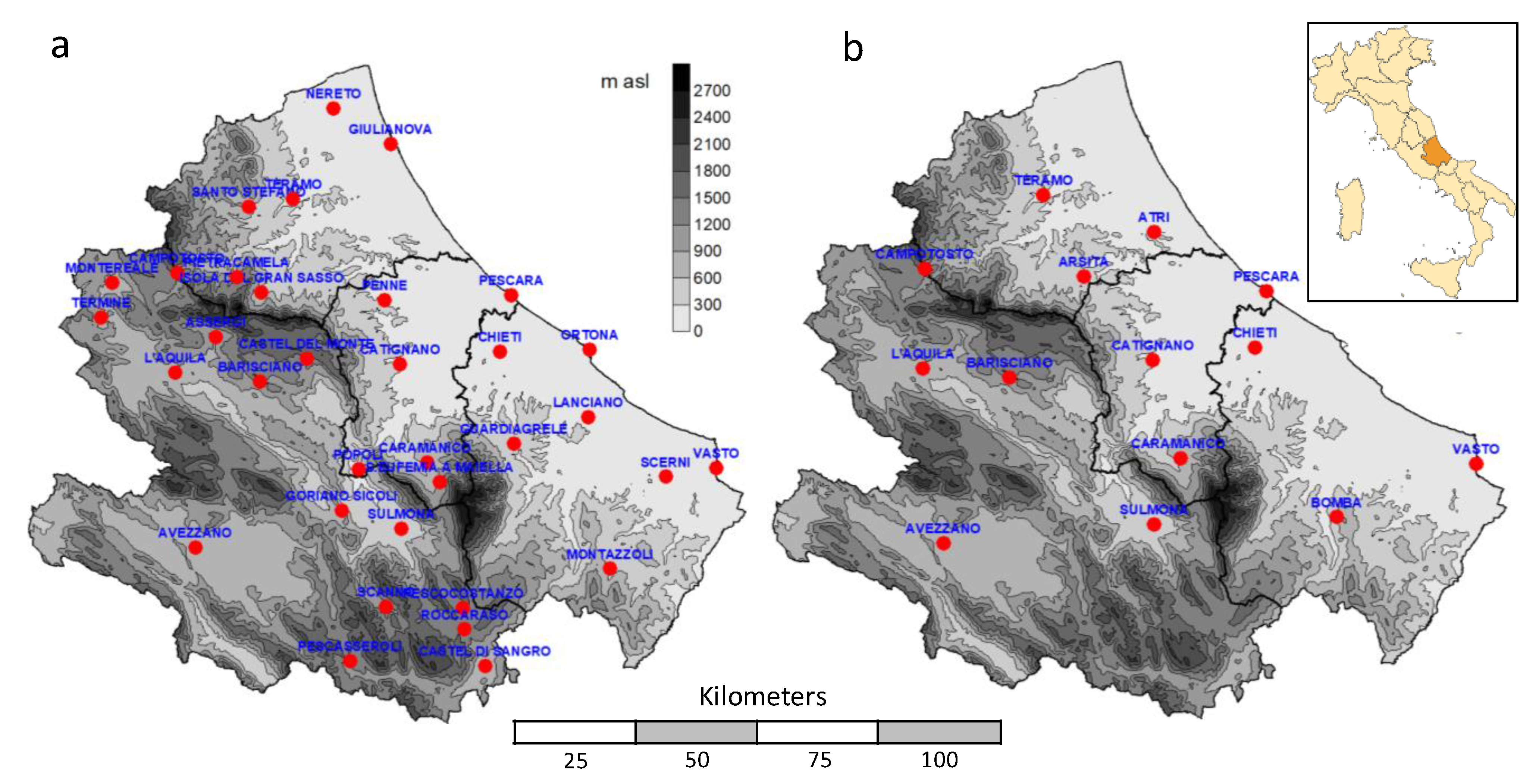
2.1. Rainfall Data

The study considered the daily rainfall data of 34 stations over the period 1980–2018. The stations are quite uniformly distributed over the territory (the red points in Figure 1a). The study was conducted using data from two different precipitation data sources: a high-quality homogenized dataset of daily observed data [37] and a widely used gridded dataset, namely the E-OBS product at 0.1° degrees resolution [38], which represents the grid product with the best resolution in the region considered. In this work, we refer to the two data sources as the “point” and “grid” datasets, respectively. Although of modest extension (10,763 km2), the Abruzzo region has a significant climate spatial variability, mainly due to a complex orography and adjacency to the sea [39].
Gauge “point” daily data were mainly provided by the Regional Hydrographic Service of Abruzzo and only for the station of Avezzano are data derived from different sources (Regional Hydrographic Service of Campania, Regional Agrometeorological Center of Abruzzo, and Telespazio). This database was subjected to extensive quality check and homogenization procedures based on the Climatol library [40] to ensure the removal of outliers and the possibility of analyzing long-term trends. Full detail is given in [37].
Grid daily data were downloaded from the public E-OBS database [38] through the European Copernicus Climate Change Service website (doi.org/10.24381/cds.151d3ec6) and interpolated on the location of the 34 gauge stations by bilinear interpolation. The database collects time series from European national weather services, subjects them to extensive quality checks and blending procedures, and finally delivers a gridded daily dataset of several atmospheric variables onto a 0.1° × 0.1° regular grid. To compare the MFI, PCI, and SI indices with that of the rainfall erosivity factor R of the USLE, we also searched for 30-min rainfall data. These data are available for few stations and only after 1999. Considering the availability and completeness of the data, we selected 14 suitable stations at the Regional Hydrographic Service in the period 1999–2020. These 14 stations (as illustrated in Figure 1b) include 11 stations already considered in the daily datasets (i.e., Avezzano, Barisciano, Campotosto, Caramanico, Catignano, Chieti, L’Aquila, Pescara, Sulmona, Teramo, and Vasto) and 3 further stations (i.e., Arsita, Atri, and Bomba). Years with more than 5% missing records were discarded. The average number of years is 16.5, with minimum and maximum values of 8 and 22, respectively.
The median annual precipitation amounts of the stations were considered and obtained from both precipitation dataset is given in Figure 2. An illustration of the seasonality at each location is given in Figure S2. The two datasets depict quite similar spatial patterns with low rainfall amounts in the stations closest to the Adriatic coast. However, the grid data, derived from interpolation algorithms, present a much more reduced variability (range between 504–1085 mm) compared to point observations (range between 594–1407 mm). In particular, grid data describe a relatively regular gradient of increasing precipitation proportional to the Adriatic coast’s distance. Therefore, the grid data do not capture either precipitation peaks (corresponding to Pescasseroli, Isola del Gran Sasso and Caramanico) or the low-precipitation stations in the inland valleys of the region (as illustrated in Figure 2a). According to previous analyses [39,41], these inland stations are characterized by the typical stau-foehn effects: the air masses of Adriatic and Tyrrhenian origin, pushed inwards by depression structures, discharge their humidity on the reliefs on the arrival side, and reach the intramountain areas depleted of precipitation.

2.2. Calculation of the Indices MFI and PCI, and of the USLE Erosivity Factor R

For each year, the Modified Fournier Index (MFI) [6] was computed as:
M F I = i = 1 12 ( p i 2 P )
where pi is the cumulated precipitation of the month i (i = 1, …, 12) and P is the cumulated annual precipitation. As explained in the introduction, there are several studies where MFI is adopted as an erosivity index. The index was also used in large-scale soil erosion risk assessments, such as in the Corine project [42]. One of the most commonly adopted classification criteria is reported in Table 1 [21,42]. MFI increases with both total annual precipitation and seasonality (also called “concentration”).
The Precipitation Concentration Index (PCI) proposed by [7] can be computed according to the following equation:
P C I = i = 1 12 ( p i 2 P 2 )
Therefore, PCI can also be computed as MFI/P. PCI ranges from 8.3% (completely uniform precipitation during the months) to 100% (precipitation concentrated in a single month). The classification of PCI given in Table 1 is taken from Lukic et al. [24] and is very similar to that originally proposed by [7].
The Seasonality Index (SI) [8] is defined as:
S I = 1 P i = 1 12 | p i P 12 |
The commonly used classification criteria of SI are given in Table 1 [43]. Both PCI and SI are often considered together with MFI in the literature to improve the interpretation of the results.
The USLE erosivity factor R (MJ mm ha−1 h−1 year−1) was computed for the 14 stations indicated in Section 2.1 following the procedure indicated by Wischmeier and Smith [2]:
R = 1 N j = 1 N [ k = 1 m ( E ) ( I 30 ) k ] j  
where (I30)k (mm h−1) is the maximum rainfall intensity of the storm k in a period of 30 min, E (MJ ha−1) is its total kinetic energy, m is the number of storms in the year j, and N is the number of years. An individual storm is preceded and followed by 6 h or more of no rain, moreover, in Equation (4), only storms with a total rainfall amount ≥ 12.7 mm or with at least 6.35 mm in 15 min are considered.
The total storm kinetic energy is computed as:
E = i = 1 n e i h i
where n is the number of time segments in the storm, hi (mm) is the rainfall depth for each increment i, and ei (MJ ha−1 mm−1) is the energy per unit rainfall [44,45]:
{ e i = 0.119 + 0.0873 l o g 10 I i , I i     76   mm   h 1 e i = 0.283 ,     I i > 76   mm   h 1
where Ii (mm h−1) is the rainfall intensity in the increment i.

3. Results

3.1. Relationships between Rainfall Erosivity Factor R and MFI, PCI, and SI

Before analyzing the spatio-temporal behavior of the MFI, PCI, and SI indices, we evaluated the relationships between the mean annual rainfall erosivity factor R (MJ mm ha−1 h−1 year−1) and the mean annual value of those indices for the 14 stations indicated in Figure 1b.
Figure 3 shows the scatter plots of the mean R vs. the mean value of the indices (MFI, PCI, and SI, respectively); the regression lines with the corresponding coefficient of determination are also reported inset.
From Figure 3a, it is evident that the mean values of MFI and R are highly correlated in the Abruzzo region. Based on the Student’s t test, the regression line’s slope presented in Figure 3a is significantly different from 0 (α = 0.01). The coefficient of determination (R2 = 0.83) indicates that the regression line explains a large part of R variance. The Root Mean Square Error (RMSE) of this model is 220.2 MJ mm ha−1 h−1 year−1. A high correlation between MFI and R was already observed in Abruzzo region [16]. However, the linear model obtained in the present analysis is more reliable due to the higher number of stations considered (14 instead of 9) and the more extended time series. Moreover, in [16], the R calculation was based on the RUSLE approach [4], which tends to underestimate the energy associated with medium-low intensity rainfall events [45]. In some literature, the relationship between R and MFI was modeled by means of power models [13]. For our data, the power model has equation R = 2.42·MFI1.41, whose exponent is equal to that obtained by [13]. However, the coefficient of determination is only slightly better than the linear model (R2 = 0.84), and the RMSE is higher (RMSE = 256.4 MJ mm ha−1 h−1 year−1).
The relationships obtained for PCI and SI (Figure 3b and 3c, respectively) indicate only a slight positive correlation between these indices and R. The scatterplots are also very similar as a consequence of the very high correlation between PCI and SI (r = 0.94). Based on the Student’s t test, only the relationship obtained for PCI can be considered significant at the 0.1 significance level. For the model of Figure 3b, the RMSE is 473 MJ mm ha−1 h−1 year−1, therefore much higher than those obtained for MFI-based models.
Two models of multiple regression of R were also tested, the first as a function of MFI and PCI (Equation (7)), the other as a function of MFI and SI (Equation (8)). These multiple regression models have the following equations, respectively:
R = 18.78 · M F I + 173.14 · P C I 2323.47   ( R 2 = 0.91 )
R = 19.12 · M F I + 2905.09 · S I 1803.29   ( R 2 = 0.90 )
In both models, the independent variables are all significant and not significantly correlated. Based on the corresponding RMSE (163.6 and 169.6 MJ mm ha−1 h−1 year−1, respectively), the model of Equation (7) can be considered the best performing.
This preliminary analysis demonstrates that in the region considered, a model based on both MFI and PCI, which only relies on monthly rainfall data, provides reliable estimates of the mean annual R.

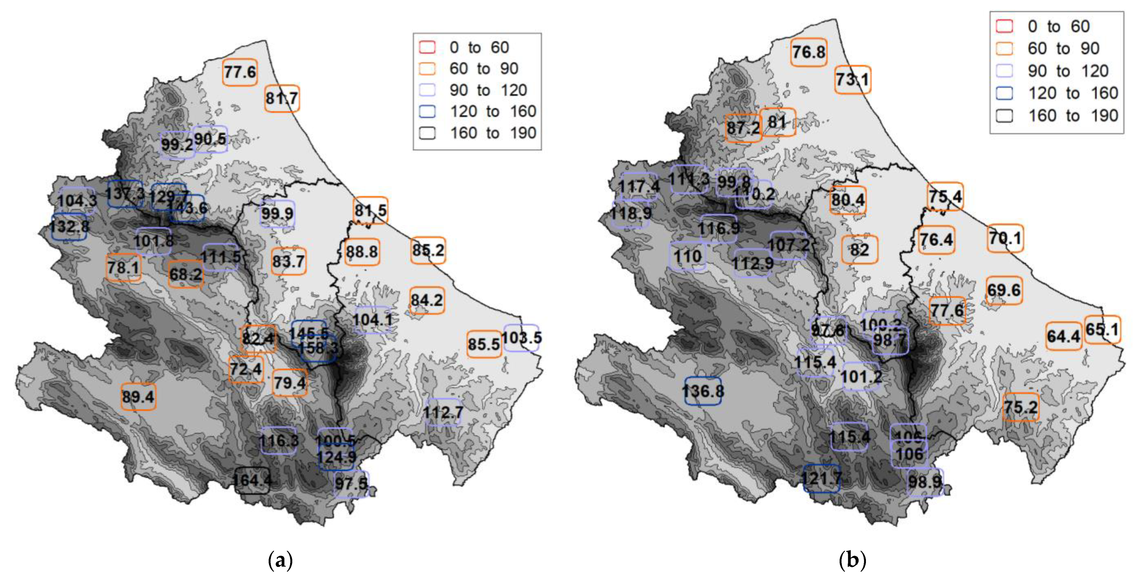
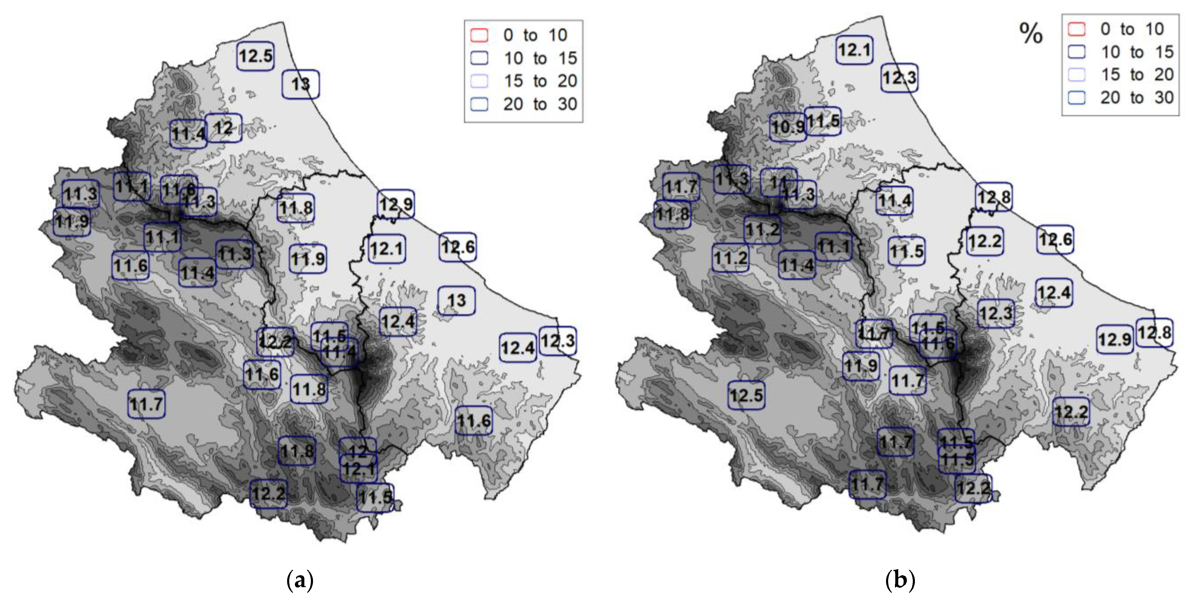
3.2. Spatial Variability of MFI, PCI, and SI

The median values of MFI, based on the point and E-OBS datasets, are shown in Figure 4. The colors associated with each station correspond to the five classes of MFI (as illustrated in Table 1). The MFI spatial pattern recall that of precipitation (as illustrated in Figure 2) with lower values along the coast and in inland valleys, demonstrating that in the region, the MFI index (and therefore, erosivity) is influenced more by the cumulative annual rainfall than by its distribution throughout the year. According to the classes presented in Table 1, Figure 4 shows that the erosive risk can be defined as low or moderate in about half of the years (the median values are reported).
The comparison between Figure 4a,b shows only an apparent agreement between the median MFI values obtained from the two datasets. The differences can be appreciated by the confusion matrix of Table 2, which indicates that the classification agreement based on the median MFI is only 41%. It was also found that the disagreement increases with the station’s altitude: for the 20 stations with elevation ≥ 500 m asl, the classification agreement is only 30% as opposed to 57% for the rest of the stations.
As regards PCI (as illustrated in Figure 5), all stations’ median values fall in the moderate class (as illustrated in Table 1), both considering the point and the grid dataset. The modest variability of PCI at a regional level contributes to the agreement, which remains also considering the maximum (instead of median) values of the series.
The seasonality index SI (as illustrated in Figure 6) has median values mainly falling in the 3rd class “Rather seasonal with a short drier season” (as illustrated in Table 1) with a very high agreement (94%) between the two datasets. The elevation doesn’t affect the agreement, while it varies considerably as the severity of SI values increases; in fact, the agreement between the classifications obtained from the two datasets reduces to 82% and 35% for the 3rd quartile and maximum, respectively.

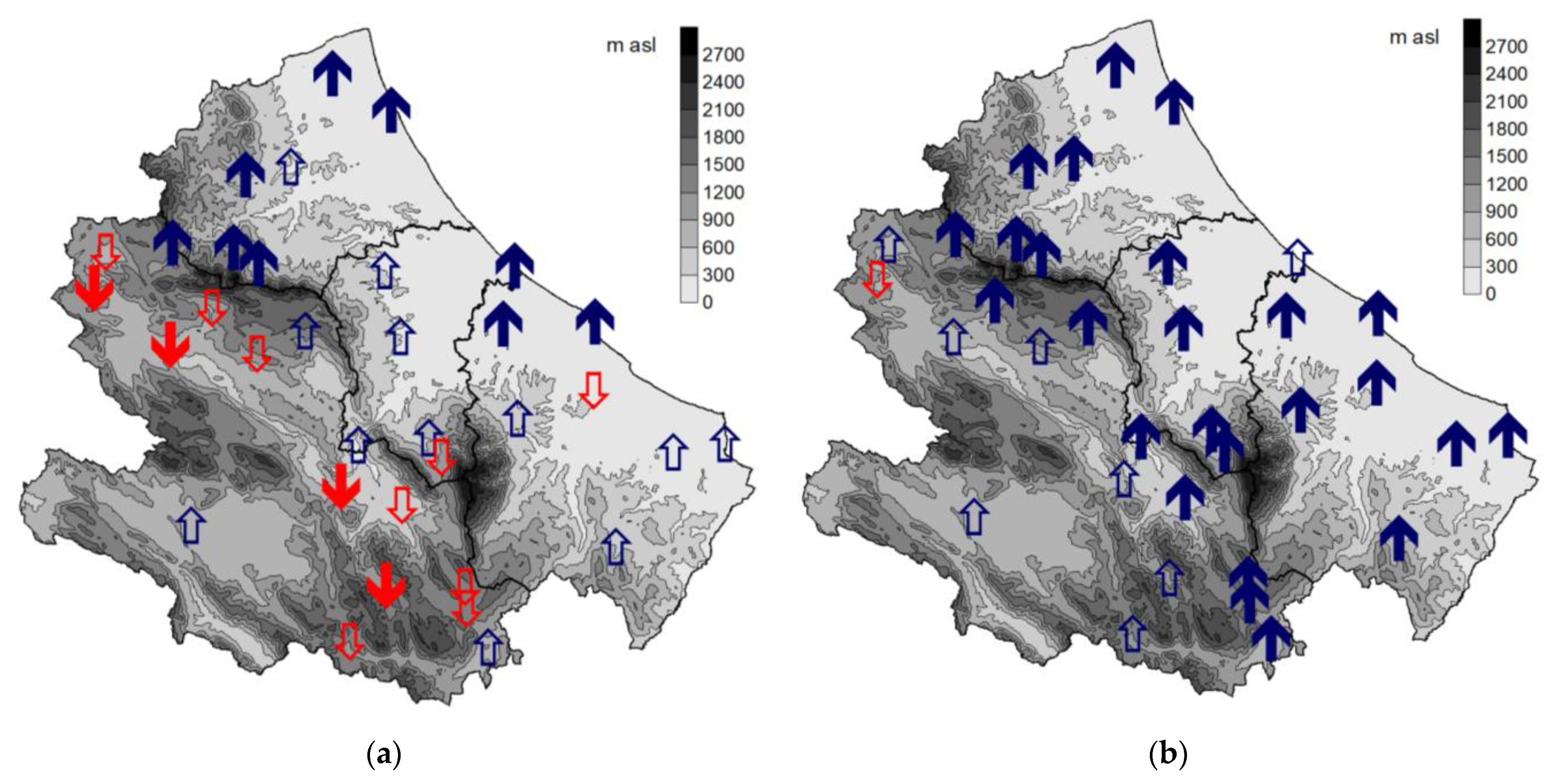
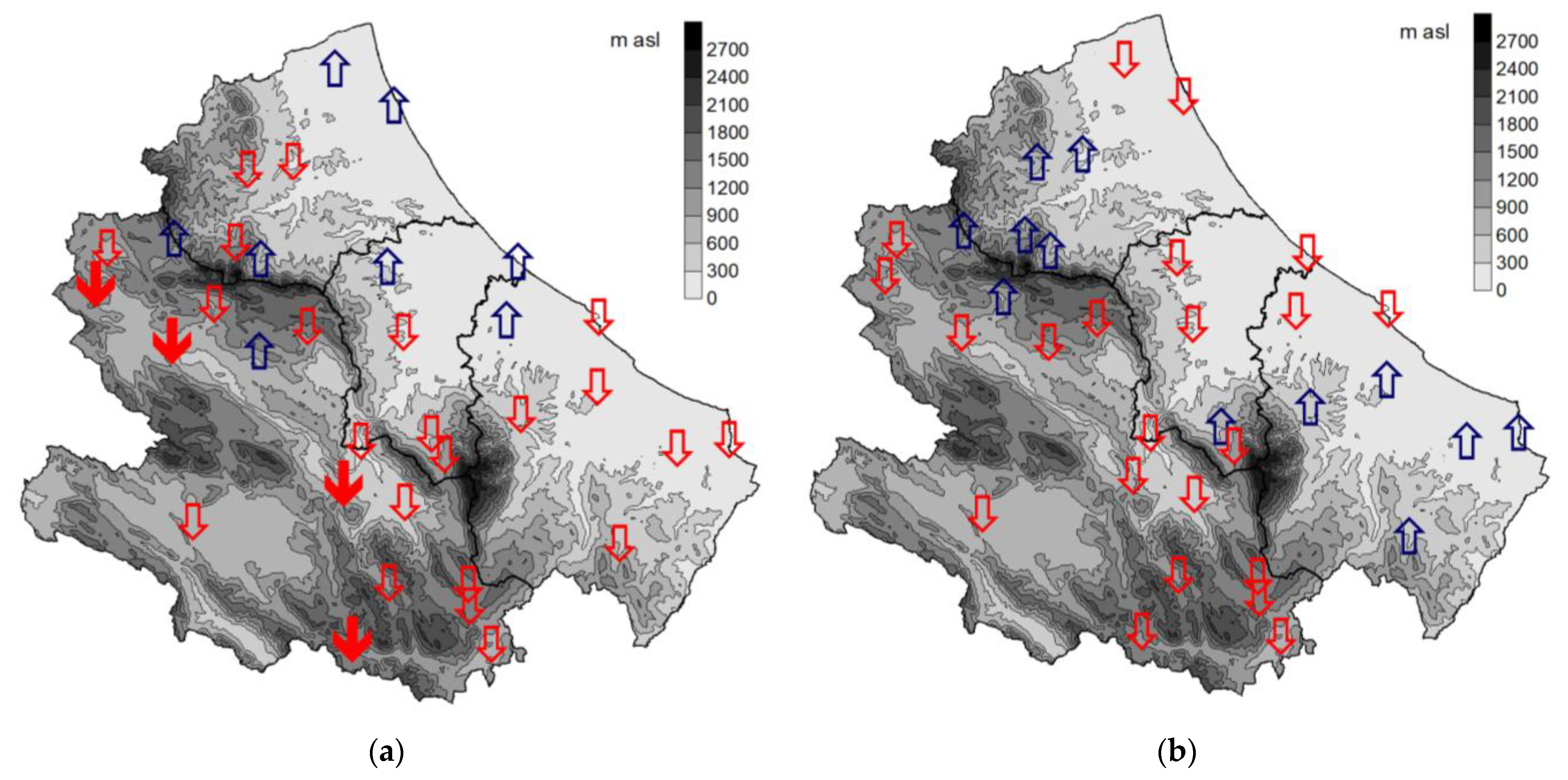
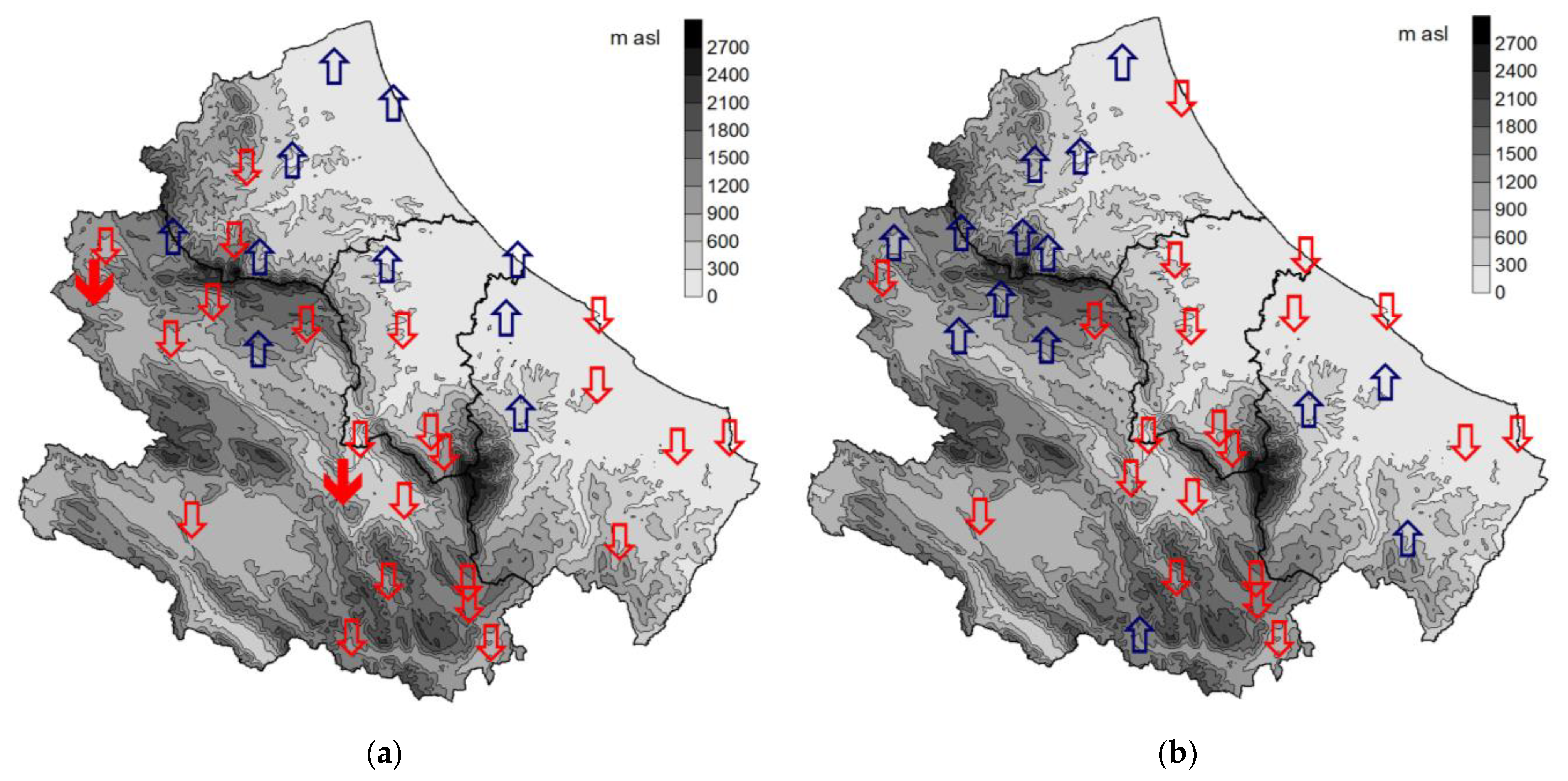
3.3. Trend Analysis of MFI, PCI, and SI

The spatial results of the trend analysis based on the Mann–Kendall test (see Appendix A for reference) are given in Figure 7, Figure 8 and Figure 9 for MFI, PCI, and SI, respectively. For MFI, the analysis of the results based on the point dataset indicates prevailing increasing tendencies in the areas closest to the coast and prevailing decreasing tendencies in the internal area. Increasing significant trends (α = 0.1) are detected in only nine stations in the northeast, while significant negative trends characterize four stations in the internal areas.
The analysis of the results obtained from grid data (as illustrated in Figure 7b) indicates widespread MFI increments, which are significant in most cases (25 out of 34 stations). A certain climatic differentiation between the stations closest to the coast and the inland ones is appreciable, but the differences are much less marked than those detected with the point dataset. Therefore, the two datasets provide a quite different assessment of the MFI time trend in the region. This difference can also be appreciated by the average regional values of Theil–Sen slope estimators, which are 0.14 and 0.69 for the point and grid datasets, respectively.
As regards PCI (as illustrated in Figure 8), the analysis indicates a prevalent stationary condition in the region, with the presence of only four significant negative trends in some inland areas for the point dataset. Therefore, the two datasets provide for similar PCI information both in terms of classification (as illustrated in Figure 5) and trends (as illustrated in Figure 8).
Considerations similar to those made for PCI apply to SI (as illustrated in Figure 9). In this case, there are only two significant negative trends on the point dataset and a general agreement between the two datasets.

4. Discussion and Conclusions

The analysis reveals that, among the indices considered, MFI is the one characterized by the greatest spatial (as illustrated in Figure 4) (as and temporal illustrated in Figure 7) variability in the region. This variability greatly affects the degree of agreement between the results obtained starting from the point and grid precipitation datasets. In fact, for MFI, somewhat discordant evaluations are obtained, both for the classification (as illustrated in Figure 4 and Table 2), and for the trends present in the 1980–2018 series (as illustrated in Figure 7). For the PCI and SI indices, considering the modest variability in the region and the near absence of significant trends, there are no substantial differences in the assessments deriving from the two datasets.
The most interesting discussion therefore concerns MFI. As already highlighted in the results, the trend analysis (as illustrated in Figure 7) reveals a marked separation in the behavior of the stations closest to the coast compared to that of the internal ones. This separation is more evident for the point dataset, which should be considered more representative of the heterogeneity of the territory. In particular, the areas of the Adriatic side are characterized by increasing trends in the MFI index, while those of the Tyrrhenian side show opposite trends. This separation may be also viewed in the grid dataset, since the few stations with insignificant trends are practically all located in inland areas.
This climatic configuration of the Abruzzo region confirms previous reports. In particular, Di Lena et al. [46], whose analysis of the main components applied to the 1951–2009 series of the Standardized Precipitation Index (SPI), revealed the presence of two main patterns, the first more correlated to the coastal areas, and the second more correlated to the inland, mountainous areas. Furthermore, for the coastal pattern, there was a marked increasing precipitation trend recent decades (i.e., an increase in rainfall). This trend is also confirmed in the present study, which goes up to 2018. In fact, the significant positive trends in MFI are always associated with significant positive trends in the corresponding annual rainfall, both for the point dataset and for the grid dataset. Moreover, a previous trend analysis based on daily data over 1980–2019 [37] showed significantly positive trends of indices of extreme precipitation in the coastal part of the region, while this trend was insignificant for inland stations.
The few significant negative trends detected for MFI in inland areas (as illustrated in Figure 7a) are instead attributable to corresponding changes in the rainfall distribution mode, as reported by the corresponding negative trends of PCI (as illustrated in Figure 8a) and partly also of SI (as illustrated in Figure 9a). For these stations, there are no significant trends in rainfall, but only a reduction in the seasonal variability of the rains which therefore tends to mitigate their annual aggressiveness (i.e., MFI). This is consistent with the seasonal precipitation trends illustrated in Curci et al. [37], where a more uniform distribution along the year was found for the recent period, with the exception of summer months which are becoming drier. Despite the greater agreement between the two datasets in terms of PCI and SI, the grid dataset does not detect the aforementioned significant negative trends.
The Equation (7) model was used to evaluate the effective practical repercussions of the rain erosivity analysis conducted with the grid data. The model is used to estimate the R factor of each station based on the average values of MFI and PCI obtained from the two datasets (Rpoint and Rgrid, respectively). These R values were also used to estimate with the USLE the average annual soil loss A = R K (t ha−1 year−1) expected for a reference bare plot (slope 9%, length 22 m and tilled in the direction of the slope), where for the soil erodibility factor K (t·h·MJ−1·mm−1), an average value of 0.032 was assumed [47].
The comparison between the Rpoint and Rgrid values for each station is shown in Figure 10, where the stations are in ascending order of annual precipitation. From the comparison, it emerges that the most marked differences occur in a limited number of stations, and these are mostly situations in which Rpoint is decidedly higher than Rgrid. These stations (Campotosto, Caramanico, Isola del Gran Sasso, Pescasseroli, Pietracamela, Roccaraso, S.Eufemia Maiella, and Termine) are all located in the internal mountainous areas (as illustrated in Figure 1) and are characterized by high annual precipitation values (and therefore of MFI), which are not well captured by the grid data. For these stations, the mean difference between Rpoint and Rgrid is about 840 (MJ mm ha−1 h−1 yr−1). Excluding these stations, the regional mean values of Rpoint and Rgrid are very similar (1604 and 1595 MJ mm ha−1 h−1 yr−1, respectively). These values are consistent with the mean Italian values indicated in Panagos et al. [3].
Figure 10 also shows the interesting case of 3 stations (Goriano Sicoli, Barisciano, and Avezzano) in which Rgrid is decidedly higher than Rpoint. Also in this case, the grid data does not capture well the pluviometric anomaly characteristic of these stations, which are subject to relatively low values of average annual precipitation (and therefore of MFI) due to a typical intramountain stau-foehn phenomenon which limits the arrival of large-scale perturbations [39].
The estimate of the annual average soil loss A obviously presents the same trend shown in Figure 10, since it was obtained for a hypothesis of constant K equal to 0.032. For the same 8 stations previously highlighted, the average difference between Apoint = Rpoint·K and Agrid = Rgrid·K is 27 t ha−1 year−1, while for the rest of the stations, the average values are aligned and equal to 51.7 and 51.4 t ha−1 year−1 for Apoint and Agrid, respectively.
The results obtained here for the Abruzzo region therefore show that the grid data allow only general indications on the spatial-temporal behavior of the indices correlated to the erosion of rain R, with consequent errors in the estimation of the potential soil loss. In many cases, these are mountain valleys and slope locations where an accurate characterization of the factors influencing erosive phenomena is particularly important.
It should also be noted that indices requiring aggregated input data on a monthly scale were used in this study. For this scale, it is likely that the lower accuracy of the grid data is mitigated compared to that of the daily data due to the compensation of random errors. In the case of erosion estimation models that require daily rainfall [19], the difference between the values of R estimated from the grid and from point data would probably be more relevant.
On the other hand, the grid data represent a very valuable resource for large-scale analyses and were already used in various circumstances for evaluations on the erosivity of rain using simplified procedures and models. Examples can be found in [32,33,34,48]. As indicated in Wang et al. [36], the mismatch between grid data and gauge data as well as interpolation errors strictly depends on the differences in spatial scales. In particular, the authors [36] indicate that the two types of data lead to different probability distributions of daily rainfall. Furthermore, the grid data tends to soften extreme values and to increase the number of rainy days.
This suggests that for erosivity risk assessment and planning of interventions in regions with complex orography, it is impossible to ignore detailed and local rainfall data. The grid data may still be applicable but require preliminary validation and possibly calibration work.

Supplementary Materials

The following are available online at https://www.mdpi.com/article/10.3390/atmos12060657/s1, Figure S1. Flowchart of the data and elaborations carried out in this study. Figure S2. Distribution of precipitation aggregated by season at each of the 34 locations used in this study.

Author Contributions

Conceptualization, methodology and software B.D.L. and L.V.; formal analysis, B.D.L., L.V. and G.C.; data curation, B.D.L. and G.C.; writing and editing, B.D.L., L.V. and G.C. All authors have read and agreed to the published version of the manuscript.

Funding

This research received no external funding.

Institutional Review Board Statement

Not applicable.

Informed Consent Statement

Not applicable.

Data Availability Statement

Grid daily data were downloaded from the public E-OBS database [37] through the European Copernicus Climate Change Service website (doi.org/10.24381/cds.151d3ec6). Point data [37] are available upon request.

Acknowledgments

In this section, you can acknowledge any support given which is not covered by the author contribution or funding sections. This may include administrative and technical support, or donations in kind (e.g., materials used for experiments).

Conflicts of Interest

The authors declare no conflict of interest.

Appendix A

Appendix A.1. Mann–Kendall Nonparametric Trend Test

The null hypothesis (H0) of the Mann–Kendall test [49,50] is that no trend is present in the population from which the dataset under investigation is extracted, whilst the alternative hypothesis indicates the presence of an increasing or decreasing monotonous trend. Being nonparametric, the test is independent of the variable’s distribution and is less influenced by the presence of outliers in the time series.
The test statistic indicated by S is given by:
S = i = 1 N 1 j = i + 1 N s i g n ( y j y i )
where N is the number of observations. yi and yj are consecutive values of the variable under study. The sign function is defined as:
s i g n ( θ ) = { 1 i f   θ > 0 0 i f   θ = 0 1 i f   θ < 0
Under the null hypothesis and for N ≥ 8, S follows a normal distribution with 0 mean and a variance approximately equal to:
V A R ( S ) = N ( N 1 ) ( 2 N + 5 ) p = 1 q t p ( t p 1 ) ( 2 t p + 5 ) 18
where q is the number of tied values, and tp is the number of tied values for them pth value. The test can be finally applied making reference to the standard deviate Z
Z = { S 1 V A R ( S ) i f   S > 0   0     i f   S = 0 S + 1 V A R ( S ) i f   S < 0
The p-Value of the test is:
Z p v a l u e = 2 [ 1 Φ | Z | ]
where Φ is the cumulative probability function of the standardized normal distribution.
The Mann–Kendall test allows us to identify the existence of a monotonous trend, but does not allow its measurement; for this reason, as usually done in the literature, the nonparametric Theil–Sen slope estimator b [51,52] was used to evaluate the slope of the straight lines interpolating the data. The Zyp [53] and Kendall [54] packages of the R statistical software were respectively used to calculate the Theil–Sen nonparametric estimator and the p-value of the Mann–Kendall test.

Appendix A.2. Sen Slope

b = M e d i a n ( x j x z j 1 )   z < j
where xj and xz are two generic sequential data values.

References

  1. Dvořák, J.; Novák, L.P. Developments in Soil Science; Elsevier: Amsterdam, The Netherlands, 1994; Volume 23, p. 13. ISBN 978-0-444-98792-1. [Google Scholar]
  2. Wischmeier, W.H.; Smith, D.D. Predicting Rainfall Erosion Losses: A Guide to Conservation Planning [USA]. Department of Agriculture Handbook (USA). 1978. Available online: https://naldc.nal.usda.gov/download/CAT79706928/PDF (accessed on 20 May 2021).
  3. Panagos, P.; Ballabio, C.; Borrelli, P.; Meusburger, K.; Klik, A.; Rousseva, S.; Tadić, M.P.; Michaelides, S.; Hrabalíková, M.; Olsen, P.; et al. Rainfall erosivity in Europe. Sci. Total Environ. 2015, 511, 801–814. [Google Scholar] [CrossRef] [PubMed] [Green Version]
  4. Renard, K.G.; Agricultural Research Service, W.; Foster, G.R.; Weesies, G.A.; McCool, D.K.; Yoder, D.C. Predicting Soil Erosion by Water: A Guide to Conservation Planning with the Revised Universal Soil Loss Equation (RUSLE); USDA: Washington, DC, USA, 1997.
  5. Yin, S.; Nearing, M.A.; Borrelli, P.; Xue, X. Rainfall Erosivity: An Overview of Methodologies and Applications. Vadose Zone J. 2017, 16, 1–6. [Google Scholar] [CrossRef] [Green Version]
  6. Arnoldus, H.M.J. An approximation of the rainfall factor in the Universal Soil Loss Equation. Approx. Rainfall Factor Univers. Soil Loss Equ. 1980, 6, 127–132. [Google Scholar]
  7. Oliver, J.E. Monthly Precipitation Distribution: A Comparative Index. Prof. Geogr. 1980, 32, 300–309. [Google Scholar] [CrossRef]
  8. Walsh, R.P.D.; Lawler, D.M. Rainfall Seasonality: Description, Spatial Patterns and Change through Time. Weather 1981, 36, 201–208. [Google Scholar] [CrossRef]
  9. Abd Elbasit, M.A.M.; Huang, J.; Ojha, C.; Yasuda, H.; Adam, E.O. Spatiotemporal Changes of Rainfall Erosivity in Loess Plateau, China. ISRN Soil Sci. 2013, 2013, 1–8. [Google Scholar] [CrossRef]
  10. Bessaklia, H.; Ghenim, A.N.; Megnounif, A.; Martin-Vide, J. Spatial variability of concentration and aggressiveness of precipitation in North-East of Algeria. J. Water Land Dev. 2018, 36, 3–15. [Google Scholar] [CrossRef] [Green Version]
  11. Gregori, E.; Andrenelli, M.C.; Zorn, G. Assessment and classification of climatic aggressiveness with regard to slope instability phenomena connected to hydrological and morphological processes. J. Hydrol. 2006, 329, 489–499. [Google Scholar] [CrossRef]
  12. Renard, K.G.; Freimund, J.R. Using monthly precipitation data to estimate the R-factor in the revised USLE. J. Hydrol. 1994, 157, 287–306. [Google Scholar] [CrossRef]
  13. Yu, B.; Rosewell, C.J. Technical Notes: A Robust Estimator of the R-factor for the Universal Soil Loss Equation. Trans. ASAE 1996, 39, 559–561. [Google Scholar] [CrossRef]
  14. Taguas, E.V.; Carpintero, E.; Ayuso, J.L. Assessing land degradation risk through the long-term analysis of erosivity: A case study in Southern Spain. Land Degrad. Dev. 2013, 24, 179–187. [Google Scholar] [CrossRef]
  15. Hernando, D.; Romana, M.G. Estimating the rainfall erosivity factor from monthly precipitation data in the Madrid Region (Spain). J. Hydrol. Hydromech. 2015, 63, 55–62. [Google Scholar] [CrossRef] [Green Version]
  16. Di Lena, B.; Antenucci, F.; Vergni, L.; Mariani, L. Analysis of the Climatic Aggressiveness of Rainfall in the Abruzzo Region. Ital. J. Agrometeorol. 2013, 1, 33–44. [Google Scholar]
  17. Märker, M.; Angeli, L.; Bottai, L.; Costantini, R.; Ferrari, R.; Innocenti, L.; Siciliano, G. Assessment of land degradation susceptibility by scenario analysis: A case study in Southern Tuscany, Italy. Geomorphology 2008, 93, 120–129. [Google Scholar] [CrossRef]
  18. Ferro, V.; Giordano, G.; Iovino, M. Isoerosivity and erosion risk map for Sicily. Hydrol. Sci. J. 1991, 36, 549–564. [Google Scholar] [CrossRef]
  19. Capolongo, D.; Diodato, N.; Mannaerts, C.M.; Piccarreta, M.; Strobl, R.O. Analyzing temporal changes in climate erosivity using a simplified rainfall erosivity model in Basilicata (southern Italy). J. Hydrol. 2008, 356, 119–130. [Google Scholar] [CrossRef]
  20. De Santos Loureiro, N.; de Azevedo Coutinho, M. A new procedure to estimate the RUSLE EI30 index, based on monthly rainfall data and applied to the Algarve region, Portugal. J. Hydrol. 2001, 250, 12–18. [Google Scholar] [CrossRef]
  21. Nunes, A.N.; Lourenço, L.; Vieira, A.; Bento-Gonçalves, A. Precipitation and Erosivity in Southern Portugal: Seasonal Variability and Trends (1950–2008): Seasonal variability and trends (1950–2008). Land Degrad. Dev. 2016, 27, 211–222. [Google Scholar] [CrossRef]
  22. De Luis, M.; González-Hidalgo, J.C.; Longares, L.A. Is rainfall erosivity increasing in the Mediterranean Iberian Peninsula? Land Degrad. Dev. 2010, 21, 139–144. [Google Scholar] [CrossRef]
  23. García-Marín, A.P.; Ayuso-Muñoz, J.L.; Cantero, F.N.; Ayuso-Ruiz, J.L. Spatial and Trend Analyses of Rainfall Seasonality and Erosivity in the West of Andalusia (Period 1945–2005). Soil Sci. 2017, 182, 146–158. [Google Scholar] [CrossRef]
  24. Lukić, T.; Lukić, A.; Basarin, B.; Ponjiger, T.M.; Blagojević, D.; Mesaroš, M.; Milanović, M.; Gavrilov, M.; Pavić, D.; Zorn, M.; et al. Rainfall erosivity and extreme precipitation in the Pannonian basin. Open Geosci. 2019, 11, 664–681. [Google Scholar] [CrossRef]
  25. Elagib, N.A. Changing rainfall, seasonality and erosivity in the hyper-arid zone of Sudan. Land Degrad. Dev. 2011, 22, 505–512. [Google Scholar] [CrossRef]
  26. Valdés-Pineda, R.; Pizarro, R.; Valdés, J.B.; Carrasco, J.F.; García-Chevesich, P.; Olivares, C. Spatio-temporal trends of precipitation, its aggressiveness and concentration, along the Pacific coast of South America (36–49° S). Hydrol. Sci. J. 2016, 61, 2110–2132. [Google Scholar] [CrossRef] [Green Version]
  27. AL-Shamarti, H.K.A. The Variation of Annual Precipitation and Precipitation Concentration Index of Iraq. J. Appl. Phys. 2016, 8, 36–44. [Google Scholar] [CrossRef]
  28. Ghenim, A.N.; Megnounif, A. Spatial distribution and temporal trends in daily and monthly rainfall concentration indices in Kebir-Rhumel watershed. LARHYSS J. 2016, 26, 85–97. [Google Scholar]
  29. Zhang, K.; Yao, Y.; Qian, X.; Wang, J. Various characteristics of precipitation concentration index and its cause analysis in China between 1960 and 2016. Int. J. Climatol. 2019, 39, 4648–4658. [Google Scholar] [CrossRef]
  30. D’Asaro, F.; D’Agostino, L.; Bagarello, V. Assessing changes in rainfall erosivity in Sicily during the twentieth century. Hydrol. Process. 2007, 21, 2862–2871. [Google Scholar] [CrossRef]
  31. Capra, A.; Porto, P.; La Spada, C. Long-term variation of rainfall erosivity in Calabria (Southern Italy). Theor. Appl. Climatol. 2017, 128, 141–158. [Google Scholar] [CrossRef]
  32. Lu, H.; Yu, B. Spatial and seasonal distribution of rainfall erosivity in Australia. Soil Res. 2002, 40, 887. [Google Scholar] [CrossRef]
  33. Vrieling, A.; Hoedjes, J.C.B.; van der Velde, M. Towards large-scale monitoring of soil erosion in Africa: Accounting for the dynamics of rainfall erosivity. Glob. Planet. Chang. 2014, 115, 33–43. [Google Scholar] [CrossRef]
  34. Zhu, Z.; Yu, B. Validation of Rainfall Erosivity Estimators for Mainland China. Trans. ASABE 2015, 61–71. [Google Scholar]
  35. Bezak, N.; Ballabio, C.; Mikoš, M.; Petan, S.; Borrelli, P.; Panagos, P. Reconstruction of past rainfall erosivity and trend detection based on the REDES database and reanalysis rainfall. J. Hydrol. 2020, 590, 125372. [Google Scholar] [CrossRef]
  36. Wang, M.; Yin, S.; Yue, T.; Yu, B.; Wang, W. Rainfall Erosivity Estimation Using Gridded Daily Precipitation Datasets. Hydrol. Earth Syst. Sci. Discuss. 2020, 1–30. [Google Scholar] [CrossRef]
  37. Curci, G.; Guijarro, J.A.; Di Antonio, L.; Di Bacco, M.; Di Lena, B.; Scorzini, A.R. Building a local climate reference dataset: Application to the Abruzzo region (Central Italy), 1930–2019. Int. J. Climatol. 2021, joc.7081. [Google Scholar] [CrossRef]
  38. Cornes, R.C.; van der Schrier, G.; van den Besselaar, E.J.M.; Jones, P.D. An Ensemble Version of the E-OBS Temperature and Precipitation Data Sets. J. Geophys. Res. Atmos. 2018, 123, 9391–9409. [Google Scholar] [CrossRef] [Green Version]
  39. Vergni, L.; Todisco, F.; Di Lena, B.; Mannocchi, F. Effect of the North Atlantic Oscillation on winter daily rainfall and runoff in the Abruzzo region (Central Italy). Stoch. Environ. Res. Risk Assess 2016, 30, 1901–1915. [Google Scholar] [CrossRef]
  40. Guijarro, J.A. Climatol: Climate Tools (Series Homogenization and Derived Products); R-Package. 2019. Available online: https://CRAN.R-project.org/package=climatol (accessed on 20 May 2021).
  41. Vergni, L.; Di Lena, B.; Todisco, F.; Mannocchi, F. Uncertainty in drought monitoring by the Standardized Precipitation Index: The case study of the Abruzzo region (central Italy). Theor. Appl. Climatol. 2017, 128, 13–26. [Google Scholar] [CrossRef]
  42. CORINE Soil Erosion Risk and Important Land Resources-in the Southern Regions of the European Community-European Environment Agency. Available online: https://www.eea.europa.eu/publications/COR0-soil (accessed on 13 April 2021).
  43. Sumner, G.; Homar, V.; Ramis, C. Precipitation seasonality in eastern and southern coastal Spain. Int. J. Climatol. 2001, 21, 219–247. [Google Scholar] [CrossRef]
  44. Wischmeier, W.H. A Rainfall Erosion Index for a Universal Soil-Loss Equation. Soil Sci. Soc. Am. J. 1959, 23, 246–249. [Google Scholar] [CrossRef]
  45. Nearing, M.A.; Yin, S.; Borrelli, P.; Polyakov, V.O. Rainfall erosivity: An historical review. Catena 2017, 157, 357–362. [Google Scholar] [CrossRef]
  46. Di Lena, B.; Vergni, L.; Antenucci, F.; Todisco, F.; Mannocchi, F. Analysis of drought in the region of Abruzzo (Central Italy) by the Standardized Precipitation Index. Theor. Appl. Climatol. 2014, 115, 41–52. [Google Scholar] [CrossRef]
  47. Panagos, P.; Meusburger, K.; Ballabio, C.; Borrelli, P.; Alewell, C. Soil erodibility in Europe: A high-resolution dataset based on LUCAS. Sci. Total Environ. 2014, 479–480, 189–200. [Google Scholar] [CrossRef] [PubMed]
  48. Bosco, C.; de Rigo, D.; Dewitte, O.; Poesen, J.; Panagos, P. Modelling soil erosion at European scale: Towards harmonization and reproducibility. Nat. Hazards Earth Syst. Sci. 2015, 15, 225–245. [Google Scholar] [CrossRef] [Green Version]
  49. Mann, H.B. Nonparametric Tests against Trend. Econometrica 1945, 13, 245–259. [Google Scholar] [CrossRef]
  50. Kendall, M.G. Rank Correlation Measures; Charles Griffin: London, UK, 1975. [Google Scholar]
  51. Theil, H. A Rank-Invariant Method of Linear and Polynomial Regression Analysis. In Henri Theil’s Contributions to Economics and Econometrics: Econometric Theory and Methodology; Advanced Studies in Theoretical and Applied Econometrics; Raj, B., Koerts, J., Eds.; Springer: Dordrecht, The Netherlands, 1992; pp. 345–381. ISBN 978-94-011-2546-8. [Google Scholar]
  52. Sen, P.K. Estimates of the Regression Coefficient Based on Kendall’s Tau. J. Am. Stat. Assoc. 1968, 63, 1379–1389. [Google Scholar] [CrossRef]
  53. Bronaugh, D.; Consortium, A.W. For the P.C.I. zyp: Zhang + Yue-Pilon Trends Package. 2019. Available online: https://CRAN.R-project.org/package=zyp (accessed on 21 May 2021).
  54. McLeod, A.I. Kendall: Kendall Rank Correlation and Mann-Kendall Trend Test. 2011. Available online: https://CRAN.R-project.org/package=Kendall (accessed on 21 May 2021).
Figure 1. Maps showing orography of Abruzzo region and stations considered: (a) stations of point and grid daily rainfall datasets; (b) stations of 30-min rainfall dataset.
Atmosphere 12 00657 g001
Figure 2. Spatial distribution of median annual rainfall amounts: (a) point data; (b) grid E-OBS data.
Atmosphere 12 00657 g002
Figure 3. Scatter plots and linear regression lines of mean annual erosivity R vs. mean annual MFI (a), PCI (b), and SI (c) at 14 stations.
Atmosphere 12 00657 g003
Figure 4. Spatial distribution of median values of MFI: (a) point data; (b) E-OBS data.
Atmosphere 12 00657 g004
Figure 5. Spatial distribution of median PCI: (a) point data; (b) grid E-OBS data.
Atmosphere 12 00657 g005
Figure 6. Spatial distribution of median SI: (a) point data; (b) grid E-OBS data.
Atmosphere 12 00657 g006
Figure 7. Spatial distribution of trend in MFI series (1980–2018): (a) point data; (b) grid E-OBS data. The down arrows indicate decreasing trends, while upper arrows denote increasing trends. Solid arrows indicate significant trends (p-Value < 0.10) according to Mann–Kendall test.
Atmosphere 12 00657 g007
Figure 8. Spatial distribution of trend in PCI series (1980–2018): (a) point data; (b) grid E-OBS data. Down arrows indicate decreasing trends while upper arrows denote increasing trends. Solid arrows indicate significant trends (p-Value < 0.10) according to Mann–Kendall test.
Atmosphere 12 00657 g008
Figure 9. Spatial distribution of trend in SI series (1980–2018): (a) point data; (b) e-OBS data. Down arrows indicate decreasing trends, while upper arrows denote increasing trends. Solid arrows indicate significant trends (p-Value < 0.10) according to Mann–Kendall test.
Atmosphere 12 00657 g009
Figure 10. Comparison between mean annual erosivity factors (Equation (8)) obtained from point and grid precipitation datasets. Stations are represented in increasing order of mean annual precipitation (based on point dataset).
Atmosphere 12 00657 g010
Table 1. Classification of MFI, PCI, and SI indices.
IndexClassDescription
MFI<60Very low
60–90Low
90–120Moderate
120–160High
>160Very high
PCI<10%Uniform distribution
10–15%Moderate distribution
15–20%Irregular distribution
>20%Strongly irregular distribution
SI<0.19Precipitation spread throughout the year
0.20–0.39Precipitation spread throughout the year, but with a definite wetter season
0.40–0.59Rather seasonal with a short drier season
0.60–0.79Seasonal
0.80–0.99Markedly seasonal with a long dry season
1.00–1.19Most precipitation in 3 months
>1.20Extreme seasonality, with almost all precipitation in 1–2 months
Table 2. Confusion matrix of MFI classes assigned to 34 stations based on the median MFI value (1980–2018) by point and grid datasets. Shaded cells indicate cases for which grid and point data assign same MFI classification.
Point Dataset
LowModerateHighVery High
Grid DatasetLow8600
Moderate5670
High1001
Very High0000
Publisher’s Note: MDPI stays neutral with regard to jurisdictional claims in published maps and institutional affiliations.

