
A New Methodology for Assessing the Interaction between the Mediterranean Olive Agro-Forest and the Atmospheric Surface Boundary Layer


Abstract
:1. Introduction
2. Physical Principles and Dimensional Analysis
2.1. Dimensional Analysis
- 1.
- Physical properties: Air density , air dynamic viscosity and gravitational acceleration g.
- 2.
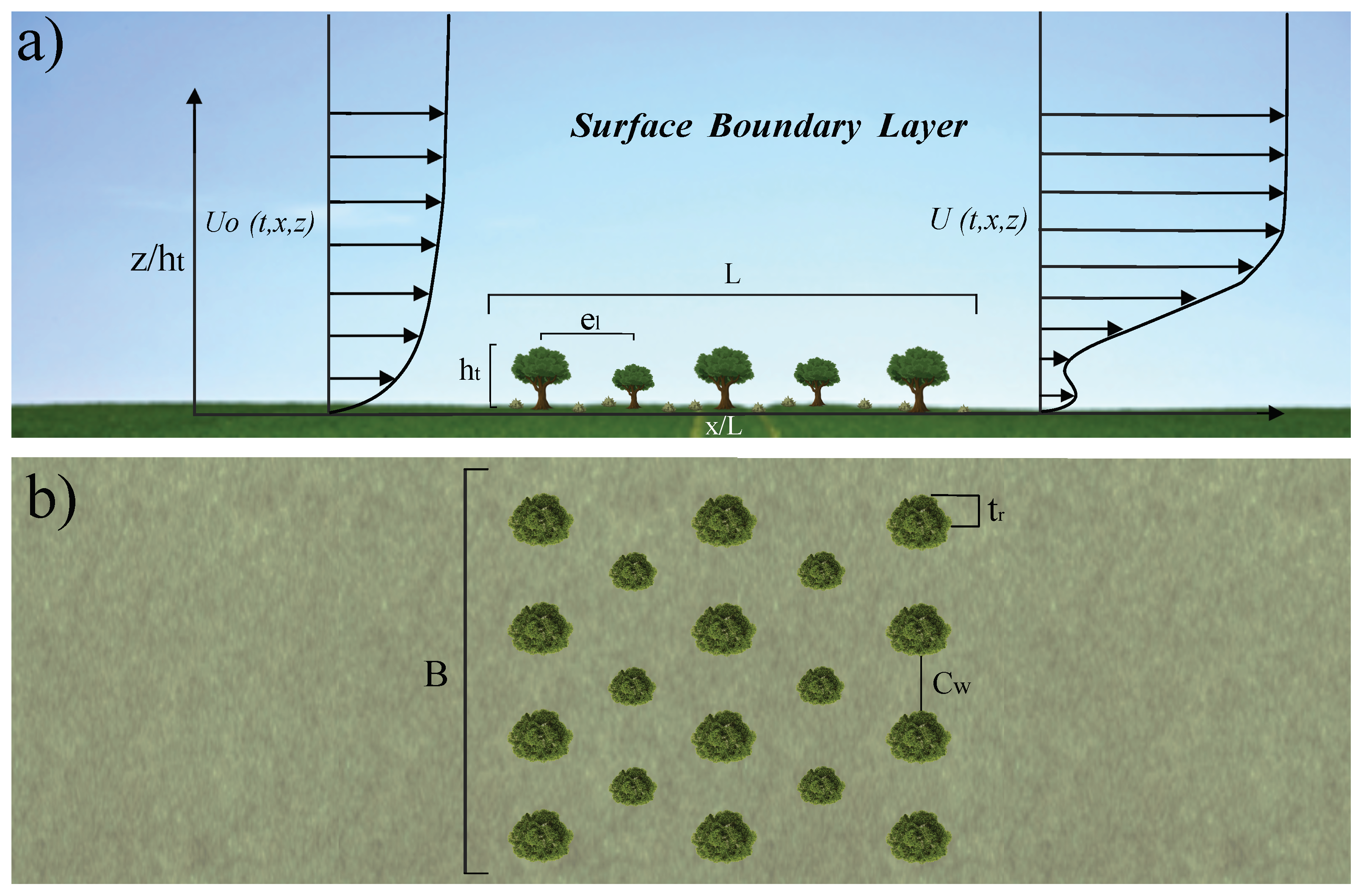
- Layout of the agro-forest (see Figure 1), including:
- Tree properties: Tree height and tree crown radius .
- Trees row properties: The streamwise distance between trees and the crosswise corridor width .
- Plantation properties: Overall length L.
- 3.
- Input: Instantaneous wind velocity profile upwind the forest, , used as reference velocity in this work, and friction velocity, , related to each other through the Von Karman expression, considering neutral atmosphere:where is the Von Karman constant and is the aerodynamic roughness length. In general, is assumed to be constant. However, for vegetation cover with discontinuities, this variable is markedly dynamic due to the natural flexibility of plants and its dependence on wind velocity and friction velocity [33]. In addition, this parameter affects the flow and modifies the vegetation itself and its surface characteristics. Performing a more formal analysis, would be selected as a variable for the dimensional analysis; however, since it is directly related to , for this specific case, is selected as input variable.
- 4.
- Output: Measured instantaneous wind velocity time series downwind the agro-forest, .
2.2. Derived Quantities
- 1.
- First kind derived quantities:
- 2.
- Second kind derived quantities:
2.3. Approach to a 3D Analysis, Aerodynamic Variables and Regimes
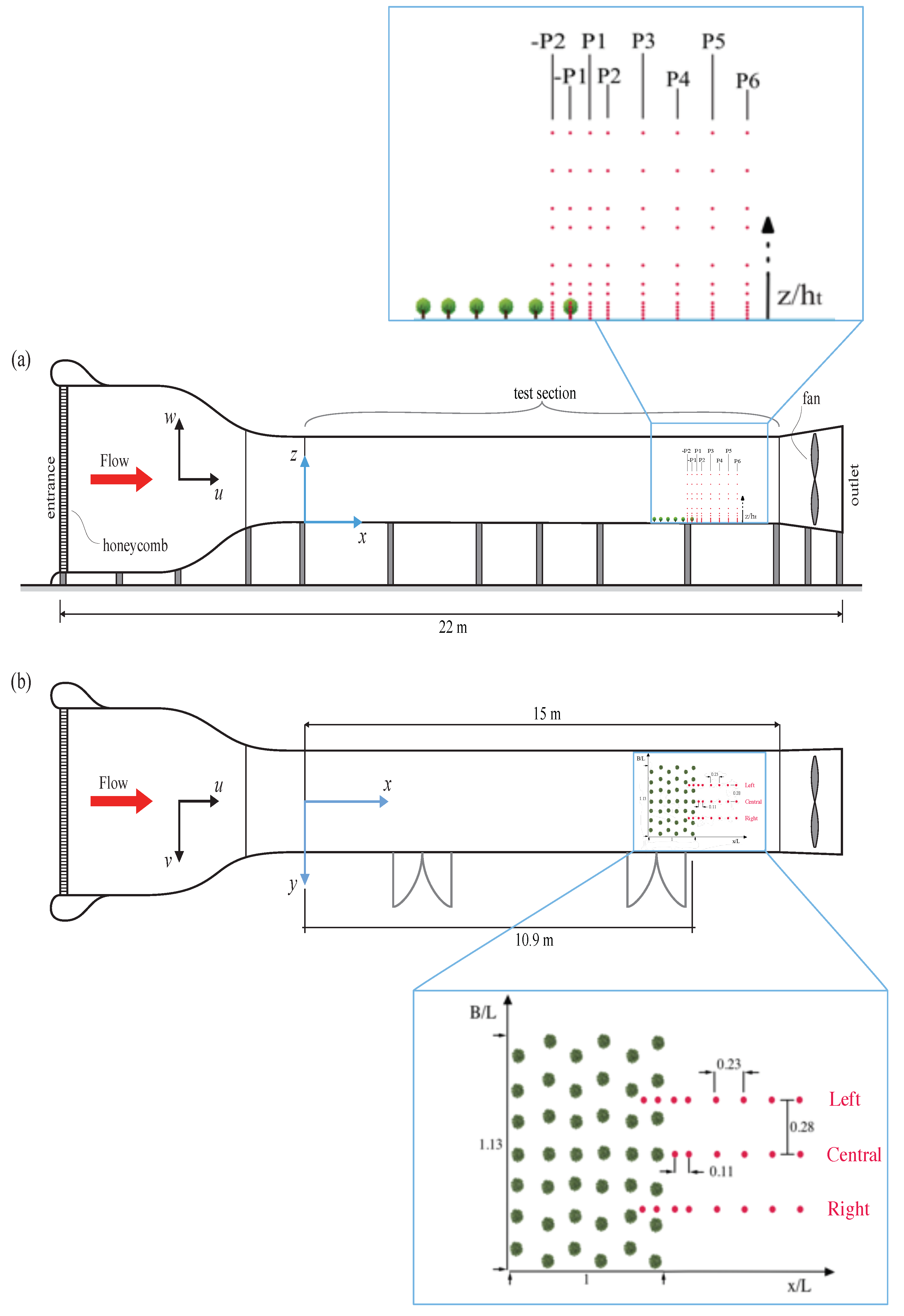
3. Experimental Setup
4. Results
4.1. Neutral Mean Flow Characteristics
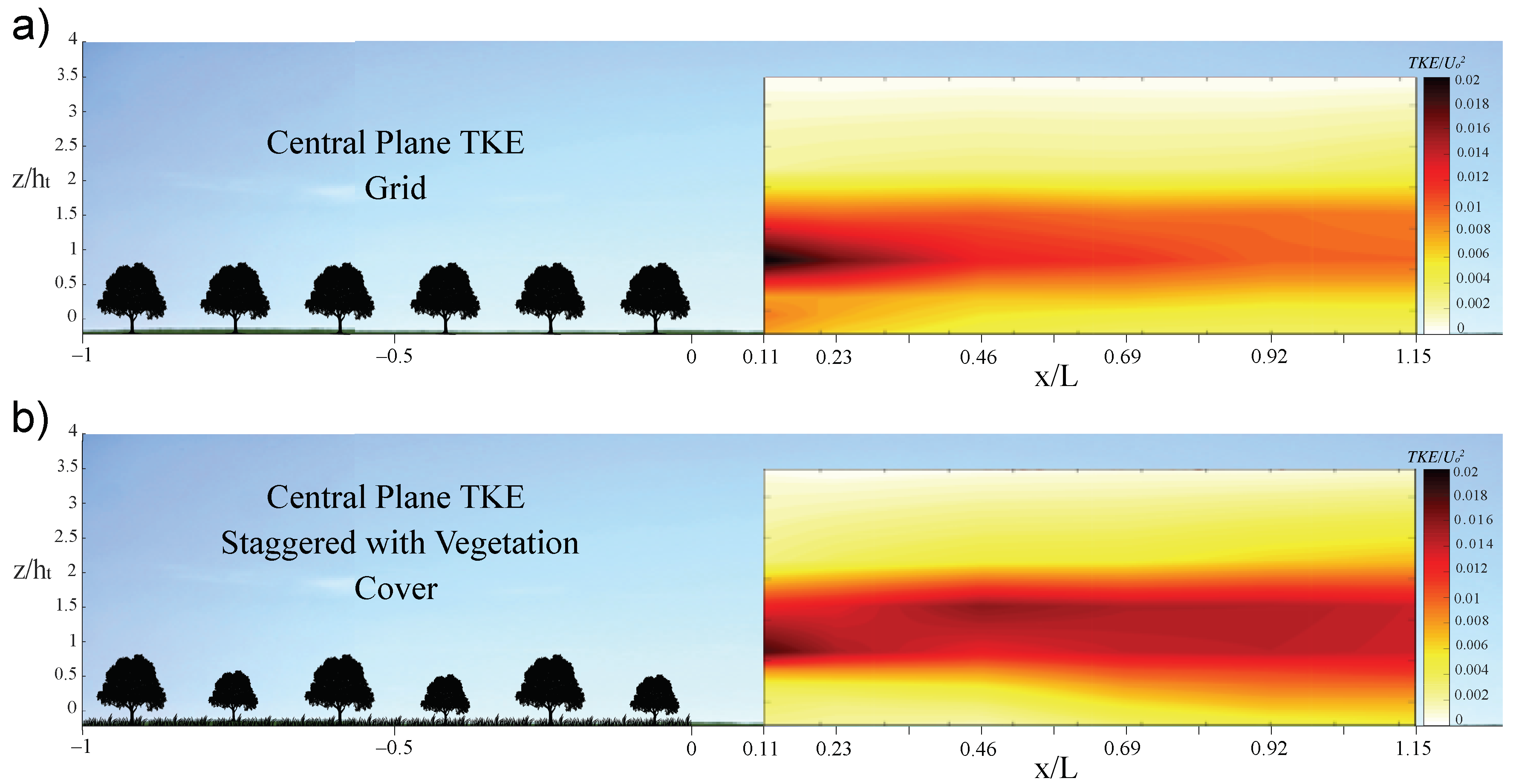
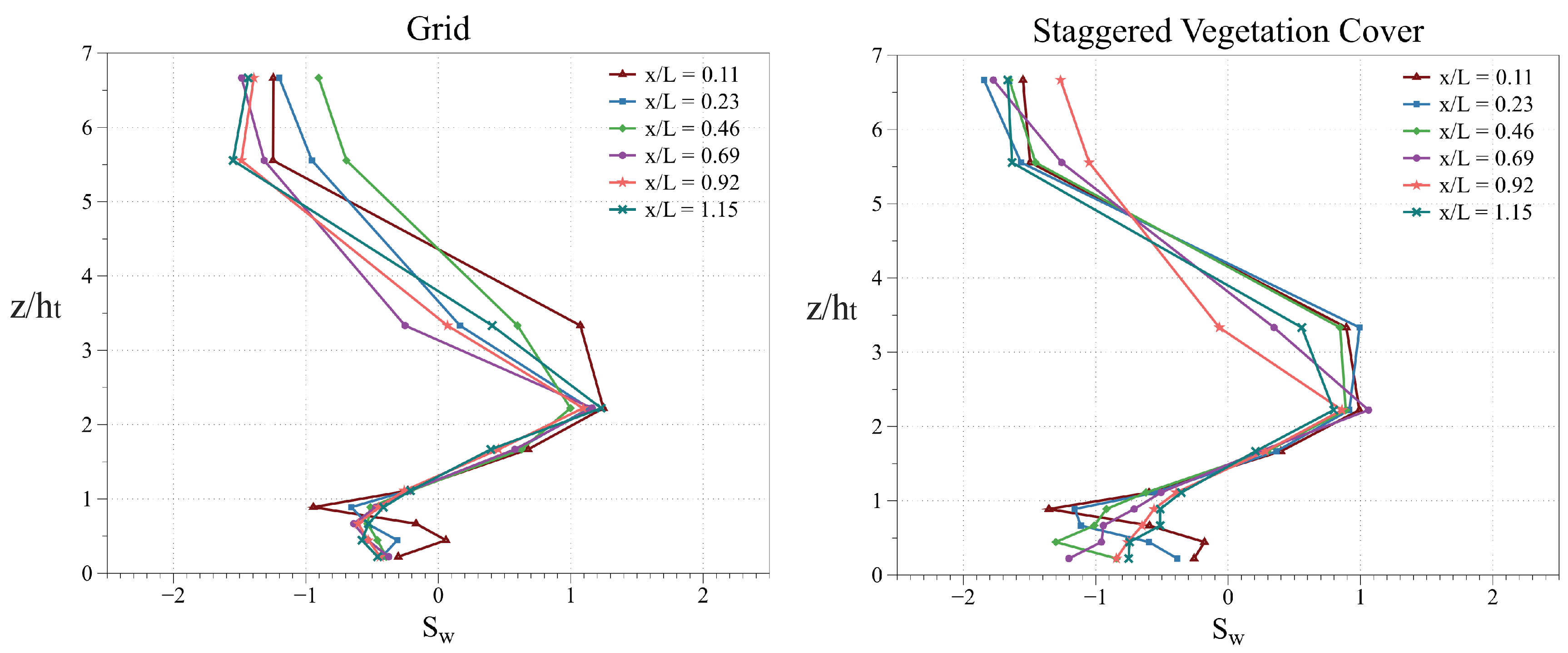
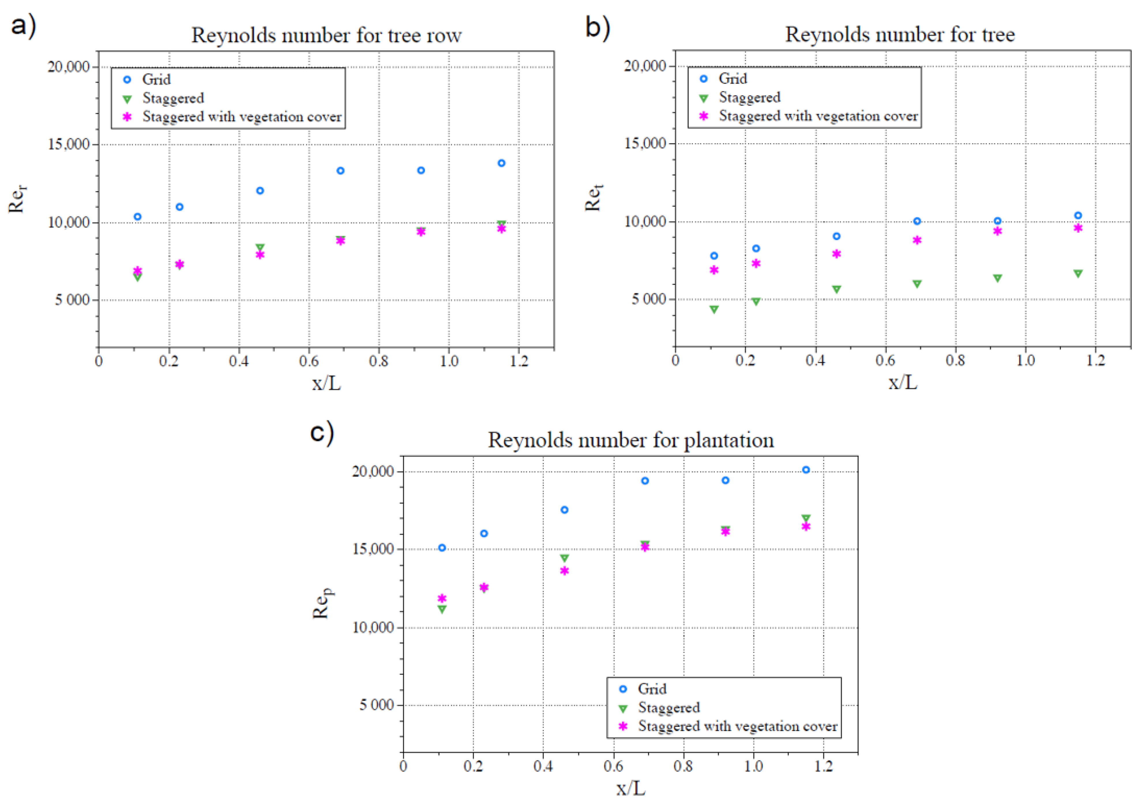
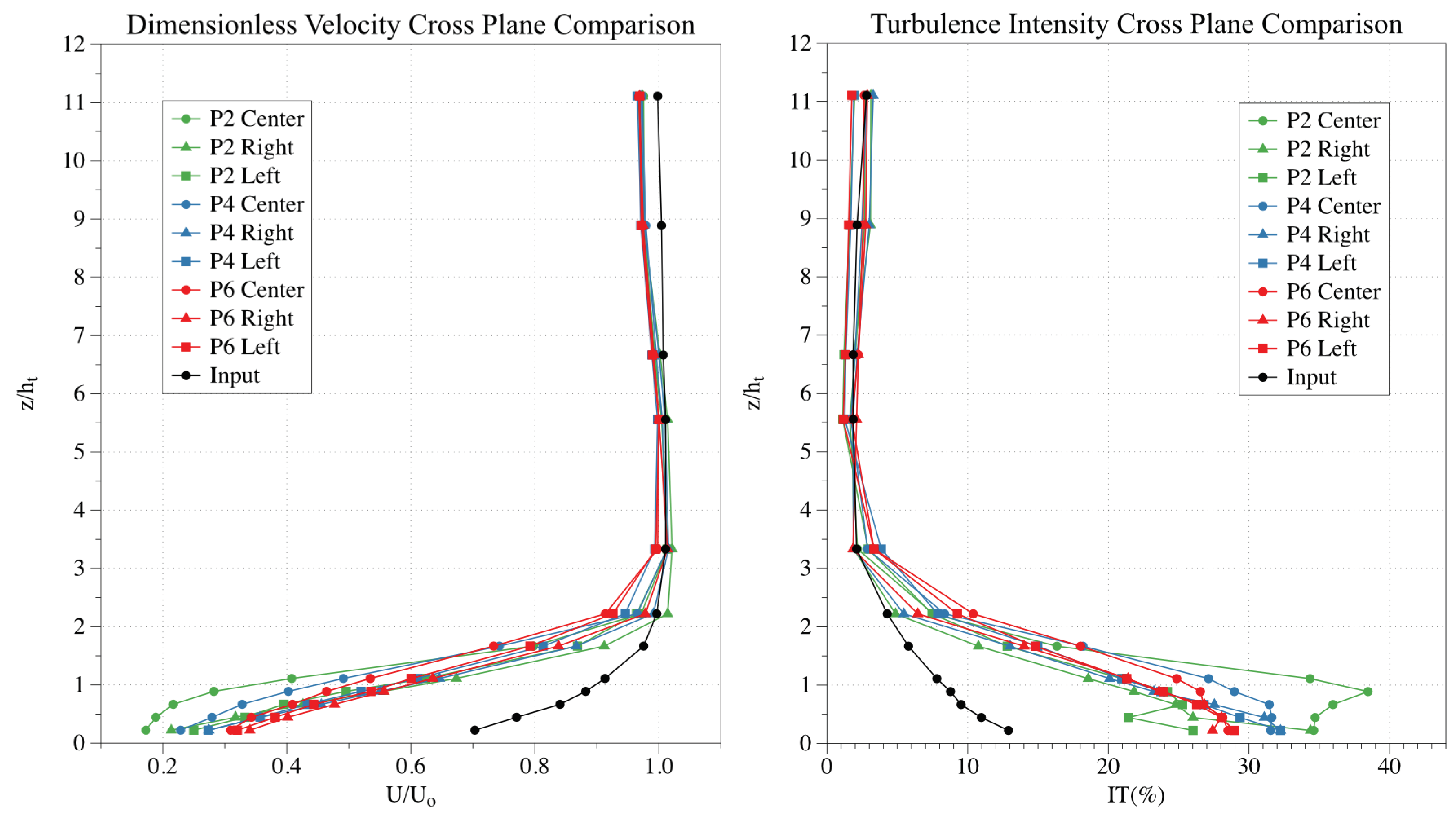
4.2. Mean Flow and Turbulence Around Olive Groves
5. Discussion
6. Conclusions
- 1.
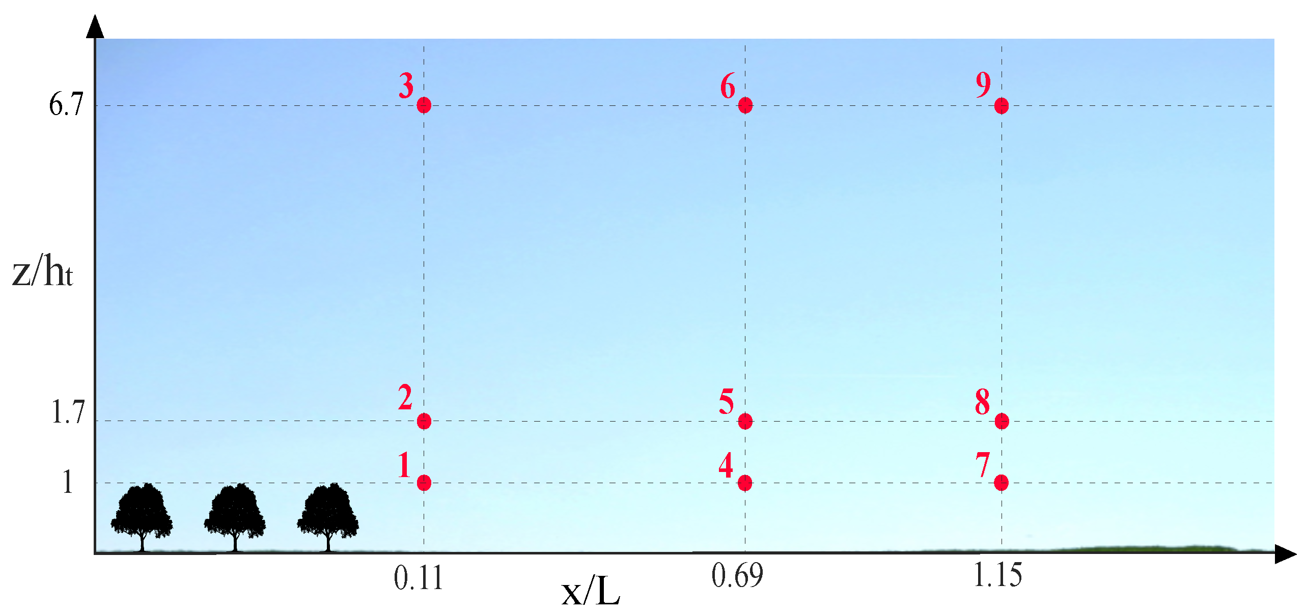
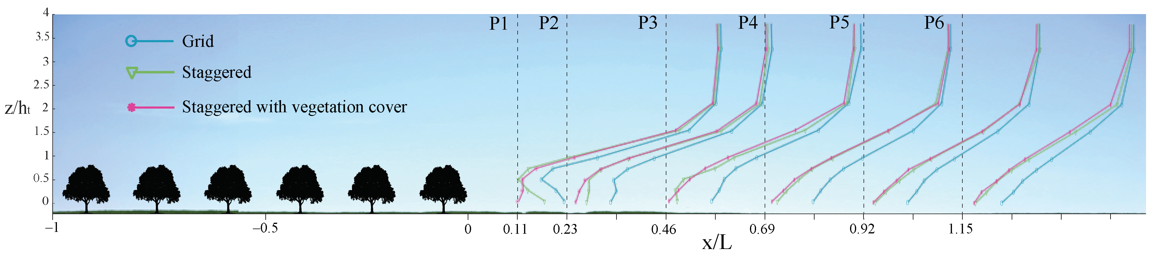
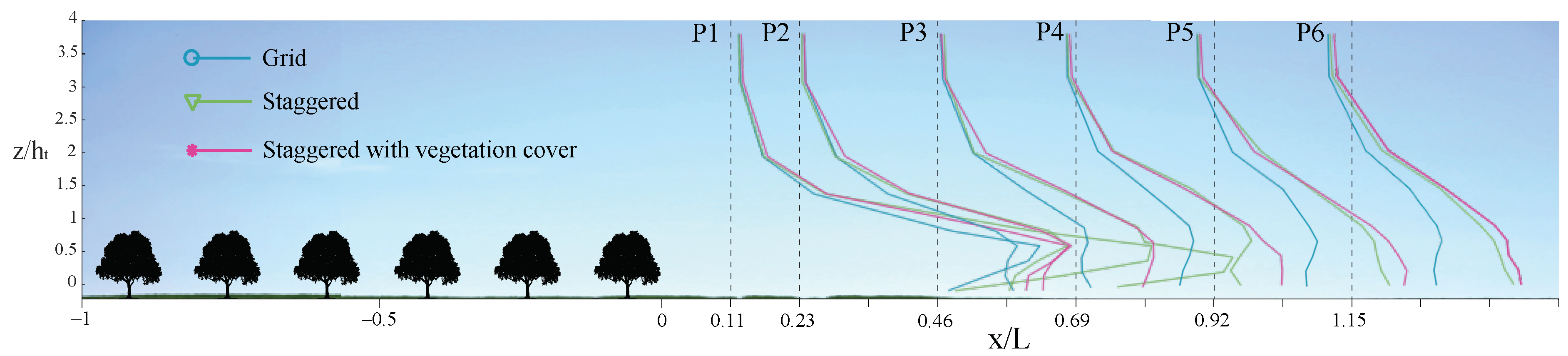
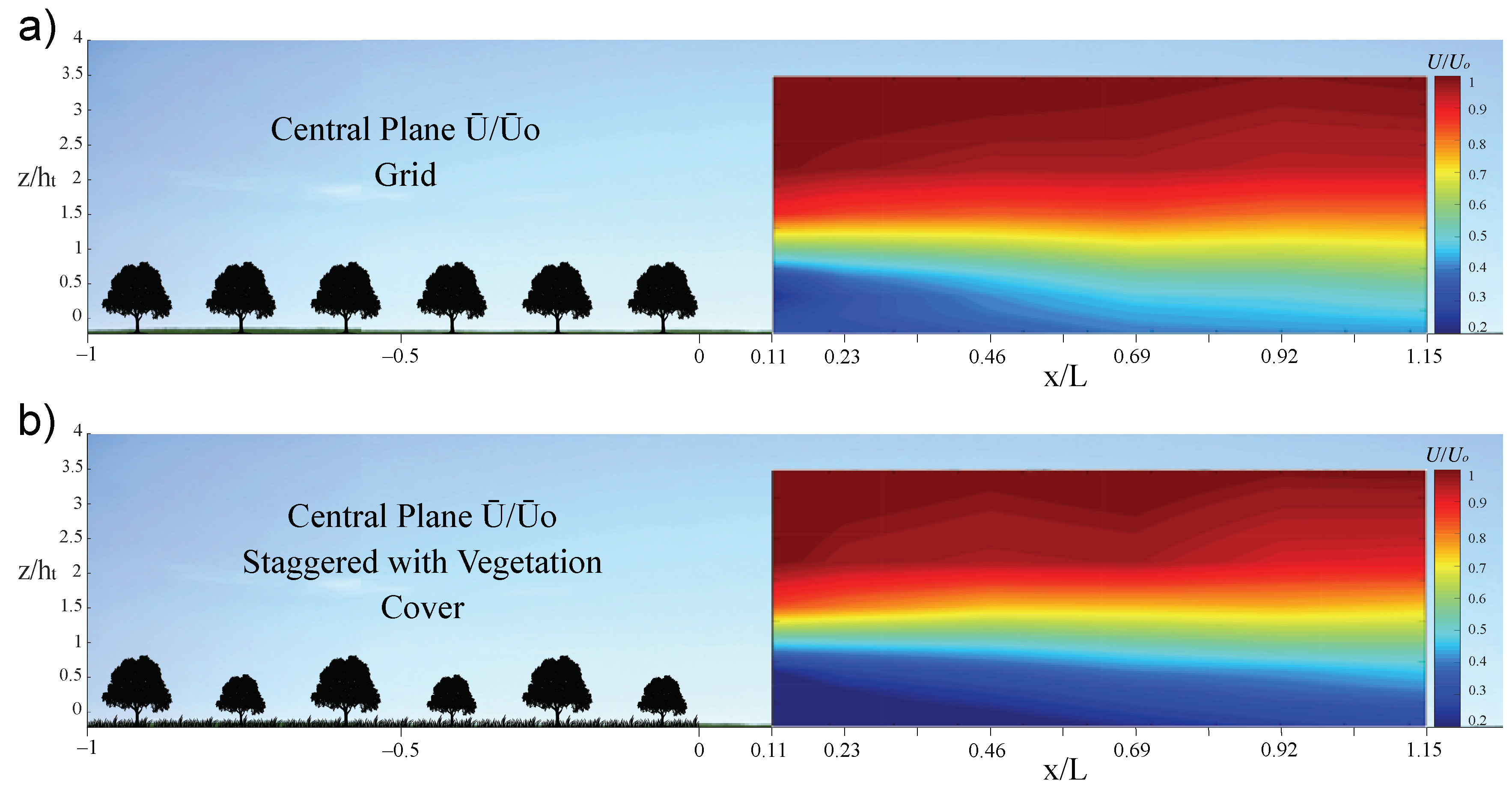
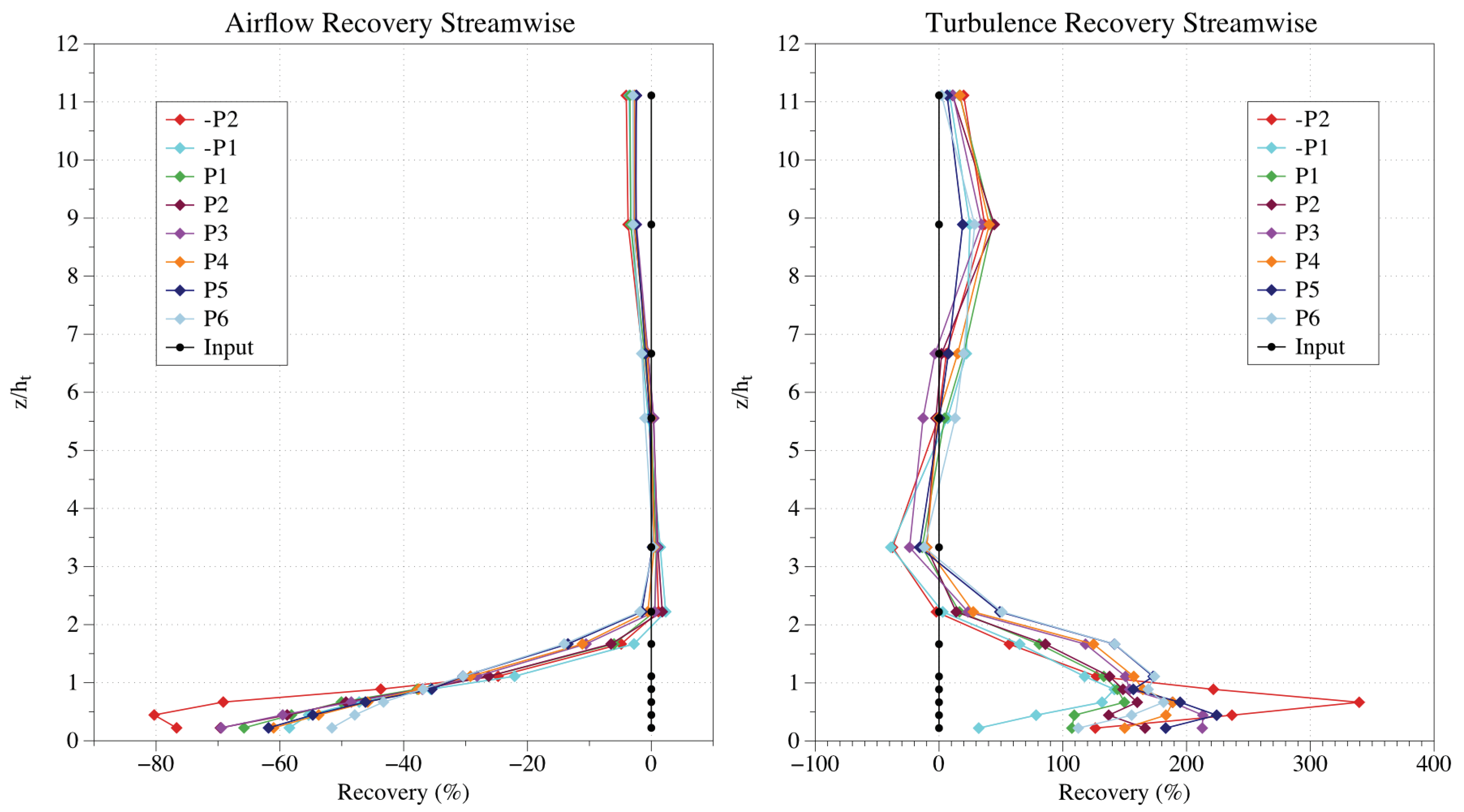
- Regarding to wind velocity profiles, a decrease is observed just behind the plantation and an acceleration of the flow up to a height , from which the profiles tend to be recovered. On the other hand, a certain acceleration is observed between trees (as could be seen in Profile -P1), at the base of the windbreak. These results are in agreement with the work of Cleugh [29].
- 2.
- Analyzing streamwise flow, vertical profiles for the different variables studied are more homogeneous and similar to each other in the case of the traditional olive grove (staggered distribution), although the levels of turbulence are higher. Moreover, the traditional olive grove shows lower streamwise variations and longer distance of air flow recovery than the intensive olive grove.
- 3.
- According to the leeward wind flow of the agro-forest, the wind velocity profile goes close to zero (but it is not zero on average) at a distance of and height approximately equal to . The vertical transition between the modified and incoming wind profiles is extended to . For the traditional olive grove, one relevant characteristic of the vertical velocity wind profile is the inflection point around . At a distance of (distance approximately equal to the total length of the plantation), the wind profile is still affected by the olive agro-forest.
- 4.
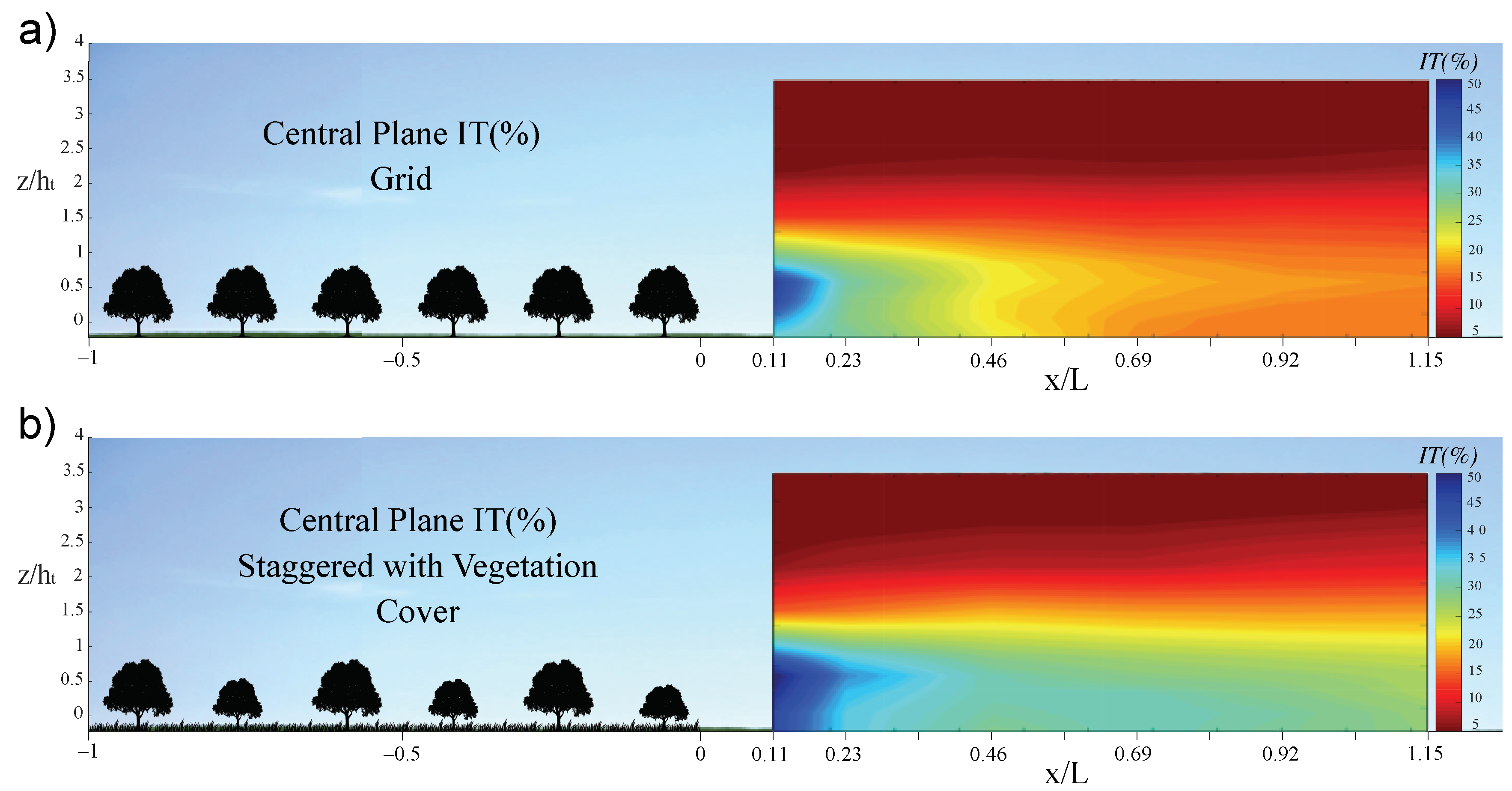
- Regarding to the turbulent characteristics, the turbulence intensity profiles grow significantly in the domain where the vertical wind profile transition occurs at , showing maximum values at approximately . Furthermore, the maximum decreases and becomes smoother; at , the exponential shape seems to almost recover, except for near the surface, depending on the layout and the cover.
- 5.
- It is concluded that, in the area next to the trees, the is similar for all the configurations; however, it is significantly higher in the case of the traditional olive grove as we move in the streamwise direction.
Author Contributions
Funding
Institutional Review Board Statement
Informed Consent Statement
Data Availability Statement
Conflicts of Interest
Abbreviations
| Atmospheric Boundary Layer | |
| B | Overall agro-forest width |
| Boundary Layer Wind Tunnel | |
| Computational Fluid Dynamics | |
| Crosswise corridor width | |
| Aerodynamic diameter of the wind tunnel | |
| Aerodynamic diameter of the plantation | |
| Aerodynamic diameter of the tree row | |
| Aerodynamic diameter of the tree unit | |
| E | Geometric scale |
| Streamwise distance between trees | |
| g | Gravitational acceleration |
| Tree height | |
| Turbulence Intensity | |
| Jensen number | |
| k | Von Karman constant |
| L | Overall agro-forest length |
| Reynolds number |
| Reynolds number for plantation | |
| Reynolds number for tree row | |
| Reynolds number of reference | |
| Reynolds number for each tree | |
| Surface Boundary Layer | |
| Skewness | |
| t | Time |
| Tree crown radius | |
| Turbulent Kinetic Energy | |
| u | Horizontal component of the velocity vector |
| Gust velocity | |
| Air friction velocity | |
| Kinematic stress | |
| Instantaneous wind velocity | |
| Input/reference wind velocity | |
| Mean wind velocity | |
| x | Horizontal distance from the agro-forest |
| w | Vertical component ow the velocity vector |
| z | Height |
| Aerodynamic surface roughness length | |
| Aerodynamic porosity | |
| Boundary layer thickness | |
| Variation rate for U | |
| Variation rate for IT | |
| Variation rate for TKE | |
| Standard deviation | |
| Variance | |
| Air density | |
| Air dynamic viscosity | |
| Air kinematic viscosity | |
| Scale ratio |
References
- Guzmán-Álvarez, J.R.; Gómez, J.A.; Rallo, L. El olivar en Andalucía: Lecciones para el Futuro de un Cultivo Milenario; Consejería de Agricultura y Pesca-Junta de Andalucía: Sevilla, Spain, 2009. [Google Scholar]
- Orlandi, F.; Rojo, J.; Picornell, A.; Oteros, J.; Pérez-Badia, R.; Fornaciari, M. Impact of Climate Change on Olive Crop Production in Italy. Atmosphere 2020, 11, 595. [Google Scholar] [CrossRef]
- Gómez, J.A. Sostenibilidad de la Producción de Olivar en Andalucía; Consejería de Agricultura y Pesca-Junta de Andalucía: Sevilla, Spain, 2009. [Google Scholar]
- Chamizo, S.; Serrano-Ortiz, P.; López-Ballesteros, A.; Sánchez-Ca nete, E.P.; Vicente-Vicente, J.L.; Kowalski, A.S. Net ecosystem CO2 exchange in an irrigated olive orchard of SE Spain: Influence of weed cover. Agric. Ecosyst. Environ. 2017, 239, 51–64. [Google Scholar] [CrossRef]
- Stull, R. Practical Meteorology: An Algebra Based Survey of Atmospheric Science; BC Campus: Victoria, BC, Canada, 2016; p. 12. [Google Scholar]
- Brunet, Y. Turbulent Flow in Plant Canopies: Historical Perspective and Overview. Bound. Layer Meteorol. 2020, 177, 315–364. [Google Scholar] [CrossRef]
- Dupont, S.; Brunet, Y.; Jarosz, N. Eulerian modelling of pollen dispersal over heterogeneous vegetation canopies. Agric. For. Meteorol. 2006, 141, 82–104. [Google Scholar] [CrossRef]
- Belcher, S.E.; Harman, I.N.; Finnigan, J.J. The Wind in the Willows: Flows in Forest Canopies in Complex Terrain. Annu. Rev. Fluid Mech. 2012, 44, 479–504. [Google Scholar] [CrossRef]
- Poëtte, C.; Gardiner, B.; Dupont, S.; Harman, I.; Böhm, M.; Finnigan, J.; Hughes, D.; Brunet, Y. The Impact of Landscape Fragmentation on Atmospheric Flow: A Wind-Tunnel Study. Bound. Layer Meteorol. 2017, 163, 393–421. [Google Scholar] [CrossRef]
- Quill, R.; Sharples, J.J.; Sidhu, L.A. A Statistical Approach to Understanding Canopy Winds over Complex Terrain. Environ. Model. Assess. 2020, 25, 231–250. [Google Scholar] [CrossRef]
- Hesp, P.A.; Dong, Y.; Cheng, H.; Booth, J.L. Wind flow and sedimentation in artificial vegetation: Field and wind tunnel experiments. Geomorphology 2019, 337, 165–182. [Google Scholar] [CrossRef]
- Gardiner, B.; Achim, A.; Nicoll, B.; Ruel, J.C. Understanding the interactions between wind and trees: An introduction to the IUFRO 8th Wind and Trees Conference (2017). For. Int. J. For. Res. 2019, 92, 375–380. [Google Scholar] [CrossRef] [Green Version]
- Moon, M.; Li, D.; Liao, W.; Rigden, A.J.; Friedl, M.A. Modification of surface energy balance during springtime: The relative importance of biophysical and meteorological changes. Agric. For. Meteorol. 2020, 284, 107905. [Google Scholar] [CrossRef]
- Nemitz, E.; Loubet, B.; Lehmann, B.E.; Cellier, P.; Neftel, A.; Jones, S.K.; Hensen, A.; Ihly, B.; Tarakanov, S.V.; Sutton, M.A. Turbulence characteristics in grassland canopies and implications for tracer transport. Biogeosciences 2009, 6, 1519–1537. [Google Scholar] [CrossRef] [Green Version]
- Arnqvist, J.; Segalini, A.; Dellwik, E.; Bergström, H. Wind Statistics from a Forested Landscape. Bound. Layer Meteorol. 2015, 156, 53–71. [Google Scholar] [CrossRef]
- Dellwik, E.; van der Laan, M.P.; Angelou, N.; Mann, J.; Sogachev, A. Observed and modeled near-wake flow behind a solitary tree. Agric. For. Meteorol. 2019, 265, 78–87. [Google Scholar] [CrossRef]
- Dupont, S.; Défossez, P.; Bonnefond, J.M.; Irvine, M.R.; Garrigou, D. How stand tree motion impacts wind dynamics during windstorms. Agric. For. Meteorol. 2018, 262, 42–58. [Google Scholar] [CrossRef]
- Albrecht, A.T.; Jung, C.; Schindler, D. Improving empirical storm damage models by coupling with high-resolution gust speed data. Agric. For. Meteorol. 2019, 268, 23–31. [Google Scholar] [CrossRef]
- Kamimura, K.; Gardiner, B.; Dupont, S.; Finnigan, J. Agent-based modelling of wind damage processes and patterns in forests. Agric. For. Meteorol. 2019, 268, 279–288. [Google Scholar] [CrossRef]
- Schindler, D.; Mohr, M. No resonant response of Scots pine trees to wind excitation. Agric. For. Meteorol. 2019, 265, 227–244. [Google Scholar] [CrossRef]
- Wei, X.; Dupont, E.; Gilbert, E.; Musson-Genon, L.; Carissimo, B. Experimental and Numerical Study of Wind and Turbulence in a Near-Field Dispersion Campaign at an Inhomogeneous Site. Bound. Layer Meteorol. 2016, 160, 475–499. [Google Scholar] [CrossRef]
- Gromke, C. Wind tunnel model of the forest and its Reynolds number sensitivity. J. Wind. Eng. Ind. Aerodyn. 2018, 175, 53–64. [Google Scholar] [CrossRef]
- Hong, Y.; Kim, D.; Im, S. Assessing the vegetation canopy influences on wind flow using wind tunnel experiments with artificial plants. J. Earth Syst. Sci. 2016, 125, 499–506. [Google Scholar] [CrossRef] [Green Version]
- Segalini, A.; Fransson, J.H.M.; Alfredsson, P.H. Scaling Laws in Canopy Flows: A Wind-Tunnel Analysis. Bound. Layer Meteorol. 2013, 148, 269–283. [Google Scholar] [CrossRef]
- Cheng, H.; Liu, C.; Kang, L. Experimental study on the effect of plant spacing, number of rows and arrangement on the airflow field of forest belt in a wind tunnel. J. Arid. Environ. 2020, 178, 104169. [Google Scholar] [CrossRef]
- Jeong, S.H.; Lee, S.H. Effects of windbreak Forest according to tree species and planting methods based on wind tunnel experiments. For. Sci. Technol. 2020, 16, 188–194. [Google Scholar] [CrossRef]
- Liu, C.; Zheng, Z.; Cheng, H.; Zou, X. Airflow around single and multiple plants. Agric. For. Meteorol. 2018, 252, 27–38. [Google Scholar] [CrossRef]
- Giometto, M.; Christen, A.; Egli, P.; Schmid, M.; Tooke, R.; Coops, N.; Parlange, M. Effects of trees on mean wind, turbulence and momentum exchange within and above a real urban environment. Adv. Water Resour. 2017, 106, 154–168. [Google Scholar] [CrossRef]
- Cleugh, H. Effects of windbreaks on airflow, microclimates and crop yields. Agrofor. Syst. 1998, 41, 55–84. [Google Scholar] [CrossRef]
- Jiménez-Portaz, M.; Chiapponi, L.; Clavero, M.; Losada, M.A. Air flow quality analysis of an open-circuit boundary layer wind tunnel and comparison with a closed-circuit wind tunnel. Phys. Fluids 2020, 32, 125120. [Google Scholar] [CrossRef]
- Sonin, A.A. The Physical Basis of Dimensional Analysis; Department of Mechanical Engineering, MIT: Cambridge, MA, USA, 2001; pp. 1–57. [Google Scholar]
- Longo, S. Analisi Dimensionale e Modellistica Fisica: Principi e Applicazioni alle Scienze Ingegneristiche; Springer Science and Business Media: Milano, Italy, 2011. [Google Scholar]
- Zhang, Q.; Zeng, J.; Yao, T. Interaction of aerodynamic roughness length and windflow conditions and its parameterization over vegetation surface. Chin. Sci. Bull. 2012, 57, 1559–1567. [Google Scholar] [CrossRef] [Green Version]
- Hogan, R.J.; Grant, A.L.; Illingworth, A.J.; Pearson, G.N.; O’Connor, E.J. Vertical velocity variance and skewness in clear and cloud-topped boundary layers as revealed by Doppler lidar. Q. J. R. Meteorol. Soc. J. Atmos. Sci. Appl. Meteorol. Phys. Oceanogr. 2009, 135, 635–643. [Google Scholar] [CrossRef]
- Manickathan, L.; Defraeye, T.; Allegrini, J.; Derome, D.; Carmeliet, J. Comparative study of flow field and drag coefficient of model and small natural trees in a wind tunnel. Urban For. Urban Green. 2018, 35, 230–239. [Google Scholar] [CrossRef]
- Jiménez-Portaz, M.; Clavero, M.; Pospisil, S.; Losada, M.A. Wind tunnel tests applied to wind energy management: Comparison of measurements in closed-circuit and open-circuit wind tunnels. In Proceedings of the 18th International Conference on Renewable Energies and Power Quality (ICREPQ’20), Granada, Spain, 1–2 April 2020. [Google Scholar]
- Longo, S. Dimensional Analysis and Physical Modelling; Springer: Parma, Italy, 2021. [Google Scholar]
- Solari, G. Wind Science and Engineering Origins, Developments, Fundamentals and Advancements; Springer International Publishing: Cham, Switzerland, 2019. [Google Scholar]
- Podhrázská, J.; Kučera, J.; Doubrava, D.; Doležal, P. Functions of Windbreaks in the Landscape Ecological Network and Methods of Their Evaluation. Forests 2021, 12, 67. [Google Scholar] [CrossRef]
- Pan, X.; Wang, Z.; Gao, Y.; Zhang, Z.; Meng, Z.; Dang, X.; Lu, L.; Chen, J. Windbreak and airflow performance of different synthetic shrub designs based on wind tunnel experiments. PLoS ONE 2020, 15, e0244213. [Google Scholar] [CrossRef] [PubMed]
- Viola, F.; Caracciolo, D.; Pumo, D.; Noto, L.V. Olive yield and future climate forcings. Procedia Environ. Sci. 2013, 19, 132–138. [Google Scholar] [CrossRef]
- Montaldo, N.; Curreli, M.; Corona, R.; Oren, R. Fixed and variable components of evapotranspiration in a Mediterranean wild-olive—Grass landscape mosaic. Agric. For. Meteorol. 2020, 280, 107769. [Google Scholar] [CrossRef]
- Paço, T.A.; Pôças, I.; Cunha, M.; Silvestre, J.C.; Santos, F.L.; Paredes, P.; Pereira, L.S. Evapotranspiration and crop coefficients for a super intensive olive orchard. An application of SIMDualKc and METRIC models using ground and satellite observations. J. Hydrol. 2014, 519, 2067–2080. [Google Scholar] [CrossRef] [Green Version]


| C | Layout | Cover | (m) | (m) | (m) |
|---|---|---|---|---|---|
| 1 | G | No | 0.09 | 0.15 | 0.04 |
| 2 | S | No | 0.07–0.09 | 0.15 | 0.02–0.04 |
| 3 | S | Yes | 0.07–0.09 | 0.15 | 0.02–0.04 |
| 3 m/s | m/s | m |
| 1 | 0.24 | 0.83 | −71.35 | 44.87 | 9.95 | 350.92 | 97.5 | ||
| 2 | 0.88 | 0.96 | −8.19 | 13.18 | 6.22 | 111.95 | 415.0 | ||
| 3 | 0.99 | 1.01 | −1.24 | 2.20 | 1.70 | 29.38 | 44.7 | ||
| 4 | 0.48 | 0.83 | −42.43 | 18.86 | 9.95 | 89.57 | 77.5 | ||
| 5 | 0.84 | 0.96 | −12.44 | 12.78 | 6.22 | 105.48 | 370.0 | ||
| 6 | 0.99 | 1.01 | −1.66 | 2.27 | 1.70 | 33.74 | 42.6 | ||
| 7 | 0.52 | 0.83 | −37.94 | 16.81 | 9.95 | 68.97 | 57.5 | ||
| 8 | 0.81 | 0.96 | −15.59 | 13.09 | 6.22 | 110.47 | 360.0 | ||
| 9 | 0.99 | 1.01 | −1.47 | 1.89 | 1.70 | 11.18 | 10.6 | ||
| 1 | 0.14 | 0.83 | −83.16 | 62.45 | 9.95 | 527.62 | 17.5 | ||
| 2 | 0.85 | 0.96 | −11.62 | 14.33 | 6.22 | 130.43 | 490.0 | ||
| 3 | 0.99 | 1.01 | −1.42 | 1.67 | 1.70 | 1.90 | 14.9 | ||
| 4 | 0.35 | 0.83 | −58.34 | 25.68 | 9.95 | 158.06 | 47.5 | ||
| 5 | 0.74 | 0.96 | −22.41 | 18.86 | 6.22 | 203.27 | 655.0 | ||
| 6 | 0.98 | 1.01 | −2.22 | 1.92 | 1.70 | 13.18 | 8.5 | ||
| 7 | 0.41 | 0.83 | −50.73 | 25.67 | 9.95 | 158.01 | 95.0 | ||
| 8 | 0.75 | 0.96 | −21.24 | 17.39 | 6.22 | 179.52 | 575.0 | ||
| 9 | 0.99 | 1.01 | −1.36 | 1.69 | 1.70 | 0.72 | 14.9 | ||
| 1 | 0.16 | 0.83 | −81.06 | 48.67 | 9.95 | 389.11 | 20.0 | ||
| 2 | 0.84 | 0.96 | −12.76 | 15.10 | 6.22 | 142.78 | 45.0 | ||
| 3 | 0.99 | 1.01 | −1.11 | 1.79 | 1.70 | 5.38 | 8.5 | ||
| 4 | 0.33 | 0.83 | −60.48 | 31.44 | 9.95 | 215.98 | 95.0 | ||
| 5 | 0.74 | 0.96 | −22.51 | 18.20 | 6.22 | 192.60 | 640.0 | ||
| 6 | 1.00 | 1.01 | −0.96 | 1.98 | 1.70 | 16.54 | 14.9 | ||
| 7 | 0.41 | 0.83 | −50.72 | 26.78 | 9.95 | 169.12 | 130.0 | ||
| 8 | 0.73 | 0.96 | −23.48 | 18.02 | 6.22 | 189.76 | 600.0 | ||
| 9 | 0.99 | 1.01 | −1.40 | 2.21 | 1.70 | 30.00 | 38.3 | ||
Publisher’s Note: MDPI stays neutral with regard to jurisdictional claims in published maps and institutional affiliations. |
© 2021 by the authors. Licensee MDPI, Basel, Switzerland. This article is an open access article distributed under the terms and conditions of the Creative Commons Attribution (CC BY) license (https://creativecommons.org/licenses/by/4.0/).
Share and Cite
Jiménez-Portaz, M.; Clavero, M.; Losada, M.Á. A New Methodology for Assessing the Interaction between the Mediterranean Olive Agro-Forest and the Atmospheric Surface Boundary Layer. Atmosphere 2021, 12, 658. https://doi.org/10.3390/atmos12060658
Jiménez-Portaz M, Clavero M, Losada MÁ. A New Methodology for Assessing the Interaction between the Mediterranean Olive Agro-Forest and the Atmospheric Surface Boundary Layer. Atmosphere. 2021; 12(6):658. https://doi.org/10.3390/atmos12060658
Chicago/Turabian StyleJiménez-Portaz, María, María Clavero, and Miguel Ángel Losada. 2021. "A New Methodology for Assessing the Interaction between the Mediterranean Olive Agro-Forest and the Atmospheric Surface Boundary Layer" Atmosphere 12, no. 6: 658. https://doi.org/10.3390/atmos12060658