Abstract
Air quality monitoring and assessment are essential issues for sustainable environmental protection. The monitoring process is composed of data collection, evaluation, and decision-making. Several important pollutants, such as SO2, CO, PM10, O3, NOx, H2S, location, and many others, have important effects on air quality. Air quality should be recorded and measured based on the total effect of pollutants that are collectively prescribed by a numerical value. In Canada, the Air Quality Health Index (AQHI) is used which is one numerical value based on the total effect of some concentrations. Therefore, evolution is required to consider the complex, ill-defined air pollutants, hence several naive and noble approaches are used to study AQHI. In this study, three approaches such as hybrid data-driven ANN, nonlinear autoregressive with external (exogenous) input (NARX) with a neural network, and adaptive neuro-fuzzy inference (ANFIS) approaches are used for estimating the air quality in an urban area (Jeddah city—industrial zone) for public health concerns. Over three years, 1771 data were collected for pollutants from 1 June 2016 until 30 September 2019. In this study, the Levenberg-Marquardt (LM) approach was employed as an optimization method for ANNs to solve the nonlinear least-squares problems. The NARX employed has a two-layer feed-forward ANN. On the other hand, the back-propagation multi-layer perceptron (BPMLP) algorithm was used with the steepest descent approach to reduce the root mean square error (RMSE). The RMSEs were 4.42, 0.0578, and 5.64 for ANN, NARX, and ANFIS, respectively. Essentially, all RMSEs are very small. The outcomes of approaches were evaluated by fuzzy quality charts and compared statistically with the US-EPA air quality standards. Due to the effectiveness and robustness of artificial intelligent techniques, the public’s early warning will be possible for avoiding the harmful effects of pollution inside the urban areas, which may reduce respiratory and cardiovascular mortalities. Consequently, the stability of air quality models was correlated with the absolute air quality index. The findings showed notable performance of NARX with a neural network, ANN, and ANFIS-based AQHI model for high dimensional data assessment.
1. Introduction
One of the most critical factors that significantly affect climate change and human health is air pollution. Many countries have been using different systems for monitoring air pollution. Thus, this area of research is of interest and very active. Several naive modeling approaches have been presented in the literature are hybrid approaches [1,2], a linear unbiased estimator [3], autoregressive integrated moving average (ARIMA) [4,5] bias adjustment [6], and principal component regression approach. Similarly, non-parametric regression [7], artificial intelligence (AI) techniques, machine learning [8], neuro-fuzzy inference systems, and autoregression feedforward ANN with genetic algorithm [9] are noble air quality modeling and control approaches. Similarly, simulation and data mining are well-known modeling tools and techniques for predicting and assessing air quality. In this context, Aggarwal et al. [10] and Bai et al. [11] have concentrated on the models used to predict the abnormality exploration in air quality. Deep learning applications (as a subset of machine learning) have recently shown considerable potential for investigating further aspects of the ecological dimensions [12,13,14]. A recent study by Sayeed et al. [15] proposed an artificial intelligence (AI) model using deep convolutional ANNs to predict 24 h ozone concentration in Texas for comparing the results of different periods in the year 2017. Munawar et al. [16] presented a case study of Lahore city of Pakistan for the prediction of an Air Quality Index (AQI) using a hybrid approach of neuro-fuzzy inference systems. Rahman et al. [17] investigated the soft computing applications of air quality modeling by reviewing and discussing the neuro-fuzzy systems, fuzzy logic, deep learning, conventional and evolutionary ANNs, and many hybrid models. Hvidtfeldt et al. [18], Ansari and Ehrampoush [19], and Liu et al. [20] expressed the exposure to pollutants causes different diseases such as respiratory diseases, asthma, type 2 diabetes, cancer, and allergies. Alimissis et al. [21], Cabaneros et al. [22], and Taylan [23] searched the air quality models playing crucial roles to evaluate the air quality problems in the atmosphere. These models can show the health conditions in the cities using domain knowledge and applying reliable and noble forecasting approaches. The advantages of these models are that they can provide early warning in case they are effectively utilized and can reduce the number of manual measurements of data acquisition substantially. As a modeling approach, ANNs provide effective, flexible, and less assumption-dependent outcomes. They have adaptive properties and can be integrated with other modeling approaches to assess and control environmental systems. The integration of ANNs and fuzzy logic models called neuro-fuzzy modeling approaches have obtained extensive attention in air quality modeling due to their adaptiveness and well-generalized performance. The different potentials of ANNs have been employed for modeling the various air pollutants, including NOx and SOx, COx, O3 [24], PM10 [25], daily precipitation and temperature using neuro-fuzzy networks [26], and PM2.5 [27] in different places all over the world. In this context, Grivas and Chaloulakou [28] used evolutionary computational algorithms such as ANNs in air quality modeling; similarly, they used genetic-algorithm-tuned ANN hybrid models for the hourly PM10 concentrations in Greece. In the time series problems, NARX with a neural network approach can be used to predict the future values of a time series ‘y(t)’ using the past values of that time series and past values of a second time series ‘x(t)’.
Similarly, as an evolutionary approach, fuzzy modeling can be used to deal with the vagueness and uncertainties of real-world problems using fuzzy ‘If-Then’ rules. A rule set is designed to control the possible relations between the input and output factors by a fuzzification process. Fuzzy modeling is a robust tool to solve complex engineering problems that are difficult to solve by traditional algebraic models. These modeling approaches encapsulate the vagueness of linguistic parameters and terms of qualitative factors. Jorquera et al. [29] demonstrated the usefulness of fuzzy logic modeling in predicting the maximum daily O3 concentration levels. The adapted neuro-fuzzy and fuzzy logic approaches have been used to model concentrations of O3 and PM10. Ghoneim et al. [30] and Zhou et al. [31] employed deep learning and deep multi-output long short-term memory ANNs models for determining the air pollutants’ concentration. Rybarczyk et al. [8] claimed that only a few review articles are available to discuss the soft computing techniques in air quality modeling [32,33,34] where it was found that these ANNs or/and deep learning techniques are mostly limited applications. The articles covering the whole spectrum of the available soft computing techniques can rarely be found.
The state of air pollution is frequently expressed by the Air Quality Index (AQI). The AQI is extensively used for air quality assessment and management [35]. The USA Environmental Protection Agency and local authorities use the AQI to provide air quality information of a location and its impact on health [36]. High AQI values mean increased pollution and high exposition of living things to health problems [37]. Sulfur dioxide (SO2 μg/m3), carbon monoxide (CO mg/m3), particular matters (PM10 μg/m3), ozone (O3, μg/m3), and nitrogen oxide NO μg/m3), and hydrogen sulfur H2S (μg/m3) are considered pollutants in the urban area. The AQI categories and their standard quality intervals are given in Table 1. These categories of AQI have been identified by fuzzy linguistic terms and their numerical intervals for air quality assessment.

Table 1.
Air Quality Index (AQI) categories [35].
In this study, initially, statistical inferencing approaches were used to examine the underlying relationship between the pollutants and their impacts on the air quality index. Equation (1) is a way to present the relationship between an air pollutant concentration and AQI. The pollutant concentration in this equation was defined as a ratio of the relevant standard.
where ci and si show the pollutant concentration and standard pollutant level, respectively. In recent years, several studies were carried out to develop air quality prediction models for launching ambient air quality standards. Numerous guidelines have been presented to set the level of air quality bounds on the emissions of pollutants [37]. On the other hand, determining and developing AQI limits using big data is a very recent work. Attention was mainly given to soft computing techniques to obtain and evaluate the big data [38] regarding the air quality models. Due to the size and complexity of big data in air quality systems, the essentials for soft computing approaches have extensively increased, particularly with the growing interests in the systems of early warning alerts and preventive actions for pollutants’ when high concentrations of pollutants are observed [23]. Recently, several attempts have been conducted to investigate air quality using machine-learning and neuro-fuzzy (ANFIS) approaches and big data analytics [10,11,15,39,40,41,42,43].
The characteristics of modeling approaches require different types of data sets. For instance, ANNs and fuzzy systems are bidirectional and need numerical and linguistic data, which are broadly discussed [44]. Similarly, fuzzy systems can organize, handle, and use vague, imprecise, and uncertain information to construct balance among different and inconsistent observations, and to use subjective and qualitative information to model complex problems [45]. As seen in Table 1, linguistic terms are employed for air quality assessment together with numerical values. The numerical data shows the upper and lower limit of pollutants that the observations have taken. Taylan et al. [46] used numerical data to train machine learning approaches and developed adaptive fuzzy models using symbolic qualitative and numerical data. Neuro-fuzzy systems integrate neural networks and fuzzy systems for developing models that have learning capabilities obtained through training processes. The goal of hybrid integration with big data is to form a more intelligent system for predicting and controlling air quality. However, applying a hybrid neuro-fuzzy system is very rare in air quality prediction and control systems. These hybrid approaches can predict air quality, evaluate the findings, and provide online information. In case of unhealthy or hazardous conditions, local authorities can take immediate actions more intelligently. In this study, the modeling method considers six major air pollutants as input parameters; SO2, CO, PM10, O3, NO, H2S, and the output parameter is the AQI. For each parameter, 1771 data were obtained, 1065 data (60%) were used for training, 353 data (20%) were used for testing, and the remaining 353 data (20%) were employed for the validation of the model.
The steps of the modeling approach are presented in detail in Section 2. The article is organized as follows: Section 2.1 describes the significant air pollution sources and their impacts on the air quality index. Section 2.2 gives the application of ANFIS in air quality modeling. The details of ANFIS modeling were presented in Section 2.3. Section 3 explains the machine learning approach for air quality estimation. Section 3.2 presents the nonlinear autoregressive with external (exogenous) input (NARX) and neural networks. The results and discussions are given in Section 4. Finally, the research ends with conclusions and references.
2. Materials and Methods
2.1. Major Sources of Air Pollution and Their Impacts on Air Quality
Several factors affect air pollution, such as dust storms, particulate matter, greenhouse gases, other gas emissions, urban growth, and transportation. The impacts of sulfur dioxide, nitrogen dioxide, and ozone cause declines in crop yields and affects human health [45]. Alternatively, ozone is caused by complex chemical reactions in the atmosphere [47]. The highest level of pollution occurs where pollutant concentrations are the greatest. The level of pollution allowed is given in Table 2, where air quality standards in Saudi Arabia, Gulf countries, and the US-EPA [37] are presented.
Table 2.
Air quality standards in Saudi Arabia, Gulf countries, and the US-EPA.
Ozone and sulfur dioxide are considered the leading causes of the low yield of crops because of the acidification of soils, lakes, and streams. When the soils are acidified, acidity and toxic aluminum move from catchments into lakes and the sea, making them highly polluted. The nitrogen disordering can acidify the soil, fertilize sensitive natural plant communities, and cause irregularity that can affect imbalance ecosystems. Figure 1a–d illustrates sulfur dioxide (a), particulate matters (b), nitrogen oxide (c), and carbon monoxide (d) on air quality. This figure shows that an increase in sulfur dioxide, particularly nitrogen oxide, raises the AQI, which means a high level of pollution and lower air quality.
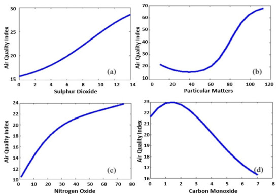
Figure 1.
The impacts of pollutants, sulfur dioxide (a), particulate matters (b), nitrogen oxide (c), and carbon monoxide (d) on air quality.
On the other hand, the effect of carbon monoxide is more complicated; this gas is a toxic air pollutant, mainly produced from vehicle emissions, and has health effects including weakness, vomiting, headaches, nausea, clouding of consciousness, coma, and, unfortunately, at high concentrations and with long enough exposure, may cause death. It also raises the AQI and reduces the air quality. However, this study aims to find out the cumulative effect of pollutants on air quality.
Air pollutants encounter the human body mainly via the respiratory system. Ozone, NO, and SO2, delicate particulate matter, and dust can affect the mucous membranes’ inflammation. These redden the eyes, inflame the pharynx and throat, affect lung functions, and weaken the immune system, which eventually causes respiratory diseases. Several symptoms may occur, such as headaches, giddiness, nausea, and pounding of the heart as the signs of extreme exposure. The US-EPA [37] standards were considered for the conversion of pollutants’ data into the indexes. As shown in Table 1, when the AQI is between zero and 50, the level of health concern is good for society. Conversely, a higher AQI means high-level pollution, which is risky for public health.
2.2. Application of ANFIS for Air Quality Modeling
An ANFIS model designed with suitable input-output parameters can depict a human expert’s behaviors to control the air quality between the predefined parameters. The model can use environmental data, produce suitable outcomes of AQI and inform authorities. An adaptive network is connected by links, where each node executes a function on incoming signals from sensory information of pollutants to produce output and specifies the direction of signal flow between the nodes [48]. In a typical network, nodes present mathematic functions modifiable by specified parameters. These parameters can impact the performance of the network and its functions. However, in this work, the mathematical functions are replaced with fuzzy rules. As shown in Figure 2, membership functions can take the place of mathematical equations and carry out their duties, which is making this approach unique and noble for air quality modeling. The complete fuzzy rules set given below, is the backbone of the expert system. Figure 2 shows the architecture of the ANFIS model for the prediction of the air quality index. An ANFIS model consisting of fuzzy if-then rules (Rs) is a fundamental tool for assessing air quality. The input parameters are Xi = {x1: Sulfur dioxide (SO2), x2: Carbon monoxide (CO), x3: Hydrogen sulfide (H2S), x4: Ozone (O3), x5: Nitrogen oxide (NOx), and x6: Particulate matters (PM10)}. The output parameter is the air quality Index (). The rules are the backbone of the ANFIS model, consisting of Gaussian MFs (μs) to depict the fuzzy linguistic terms (φs) and are presented in the rule set given below.
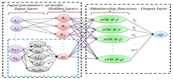
Figure 2.
The adaptive neuro-fuzzy inference (ANFIS) model architecture for air quality prediction.
It is essential to mention that there are often uncontrollable and unavoidable causes of variations in air quality. Identifying variations require dealing with air quality characteristics using linguistic terms. Collecting numerical data about the air pollutants is essential, but this will not be as meaningful as linguistic terms used to identify the air quality parameters. Because crisp numbers cannot identify some parameters, fuzzy linguistic terms might be more suitable to deal with these parameters. For instance, air quality is a linguistic variable whose values might be linguistic terms such as ‘good, healthy, unhealthy, very unhealthy, hazardous, etc.’ Due to the imprecision and vagueness in these quality measures, a trend was initiated to integrate the randomness and fuzziness for assessing environmental quality problems. In Figure 3a,c, the air quality index is plotted in three-dimensional (3D) graphs versus carbon monoxide and sulfur dioxide. Similarly, it was plotted against ozone and nitrogen oxide for Jeddah, respectively. Figure 3b,d shows that the nonlinear relation appears clearly between the input parameters and the air quality index. The 3D plots are very obliging for observing the full view of the air quality index’s output surface based on the whole span of the input parameters. The 2D and 3D plots of air quality index and regressors such as ozone, sulfur dioxide, carbon monoxide, and nitrogen oxide showed that the system was nonlinear and recommended the evolution of an intelligent approach to predict and control the air quality in a city.
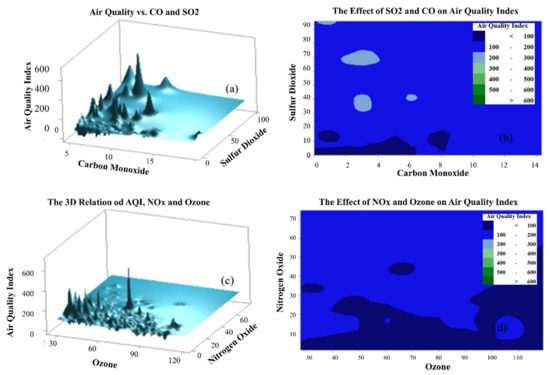
Figure 3.
The impacts of pollutants on the air quality index. (a–d) The impacts of pollutants on the air quality index.
The analysis of 3D surfaces shows that many local maximum and minimum points appear in the responses of the given parameters. Therefore, this reveals that the rise (or maximum points) in the pollutant concentration will increase the AQI and cause many negative effects. On the other hand, the local and global minimum points show where the AQI is low, and the air quality is good and healthy. Hence, a highly nonlinear relation appears between the pollutants and air quality index.
2.3. ANFIS Based Reasoning for Air Quality Prediction
The ANFIS model was established from six rules and the linguistic statements for air quality modeling and prediction. Fuzzy rules are used to map input parameters to the output. A fuzzy rule is constituted from the assertion and the conclusion parts, including linguistic variables and their term sets. Clustering analysis was carried out, and the optimal number of clusters was found to be six with a 99.9480% similarity level and 0.00104 distance level between the clusters. Therefore, the number of rules was considered equal to the number of clusters; each rule represents the characteristic of data in the cluster for identifying the AQI. Due to the nonlinearity (see in Figure 1 and Figure 3), Gaussian membership functions (MFs) (see in Figure 4 and Figure 5) were employed for the fuzzy input sets and delta functions for the output spaces. In this study, the center average defuzzification and product premise approach were employed for obtaining the outcomes of AQI, as given in Equation (2).
where R represents the number of rules in the rule base, ‘n’ denotes the number of inputs per data tuple. θ is represented in a vector form that contains the MF parameters for the rule base, ‘ci’ is the MF center, and ‘σi’ is the width of MFs () in the rule base, the Gaussian MFs were used for the rules’ premises, and the delta function is used for the conclusion part. The coefficient bi represents the point in the output space at which the output MF for the ith rule is a delta function and denotes the point in the jth input universe of discourse, where the MF for the ith rule achieves a maximum. It is essential to mention that the relative width; of the jth input MF for the ith rule is always larger than zero. Fuzzy reasoning is the crucial factor in the modeling of fuzzy set theory. For the prediction of air quality, the input membership functions, fact base, the ruleset, and the inference engine are presented in Figure 4. These fuzzy rules and the reasoning process and defuzzification are considered as the pillar of the fuzzy inference system to obtain the outcomes of the fuzzy model. Figure 4 shows the fuzzy reasoning procedure of the Sugeno fuzzy model [23] for predicting the air quality in Jeddah.
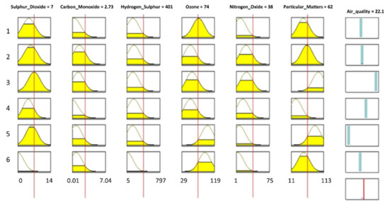
Figure 4.
Fuzzy reasoning procedure for predicting air quality.
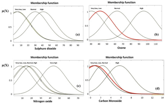
Figure 5.
Depicts the MFs and their term sets for sulfur dioxide (a), ozone (b), nitrogen oxide (c), and carbon (d).
If air pollution is considered as a space-defining by fuzzy set U, Xis is the fuzzy input parameters in this space and Yi is the fuzzy output parameter, then, the input parameters of this work are; Xis = {x1: Sulfur dioxide (SO2), x2: Carbon monoxide (CO), x3: Hydrogen sulfide (H2S), x4: Ozone (O3), x5: Nitrogen oxide (NOx), and x6: Particulate matters (PM10)}, and the output parameter is the air quality Index () which can be used for neuro-fuzzy modeling. The fuzzy linguistic term set employed for this study is φs = {good, moderate, unhealthy, very unhealthy, and hazardous}. A fuzzy model is structured by the collection of fuzzy If-Then rules. The upper and lower limits of all input parameters and output are presented in Figure 4. This figure also shows the fuzzy reasoning procedure. For instance, the upper and lower bounds of sulfur dioxide (SO2) are between 0–14 μg/m3, ozone’s (O3) is between 29–119 μg/m3, and particulate matters (PM10) is between 11–113 μg/m3, and so on. The membership functions i = 1, 2, …, n, are always parametric functions used in the fuzzy model. Figure 5a–d depicts the MFs and their term sets for sulfur dioxide (a), ozone (b), nitrogen oxide (c), and carbon monoxide in Jeddah, respectively.
- Rule 1: IF (SO2) is low and (CO) is low and (H2S) is low and (O3) is low and (NO) is low and (PM10) is low THEN The air quality is good.
- Rule 2: IF (SO2) is low and (CO) is normal and (H2S) is normal and (O3) is low and (NO) is normal and (PM10) is normal THEN The air quality is good.
- Rule 3: IF (SO2) is high and (CO) is normal and (H2S) is normal and (O3) is low and (NO) is normal and (PM10) is very high THEN The air quality is normal.
- Rule 4: IF (SO2) is low and (CO) is high and (H2S) is high and (O3) is very low and (NO) is high and (PM10) is very low THEN The air quality is unhealthy.
- Rule 5: IF (SO2) is normal and (CO) is high and (H2S) is high and (O3) is very high and (NO) is high and (PM10) is high THEN The air quality is unhealthy.
- Rule 6: IF (SO2) is very low and (CO) is very high and (H2S) is very high and (O3) is high and (NO) is very high and (PM10) is low THEN air quality is hazardous.
Appropriate separation of fuzzy input and output data spaces and a correct choice of MFs are essential to obtain a useful ANFIS model for the AQI. The MFs and the fuzzy term sets of all variables are determined based on the domain knowledge of the system parameters considered. The Gaussian MFs are identified by two parameters (c, σ), where ‘c’ denotes the MFs’ center, and ‘σ’ represents the MFs’ width. Figure 5c shows the Gaussian MFs for ‘nitrogen oxide’ and fuzzy term set ‘very high’ representing the MFs. Some other fuzzy variables and their MFs are presented in Figure 5. For example, the MF of ‘nitrogen oxide’ for the fuzzy term ‘very high’ is mathematically presented as given in Equation (3).
A big data set was used for the training, testing, and validation of the ANFIS model developed which can cover the nonlinear functional dependency between the input and output parameters. The root-mean-square error (RMSE) approach was employed for the error determination, in which ‘oi’ and ‘pi’ are the observed and predicted values of error, respectively, for the AQI. Equation (4) gives the mean square error of the ANFIS model developed for this study.
Figure 6 shows the relative error of training and testing data determined for the ANFIS model developed.
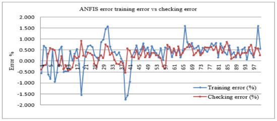
Figure 6.
The training and checking error were determined for the ANFIS model.
As seen in Figure 6, the relative errors were tolerable and the model checking performance was good. On the other hand, the average training error was found at 4.42, and the RMSE for the training data set was calculated at 5.64. Essentially, both the RMSEs were very small for the training and testing of the ANFIS model. Therefore, the developed ANFIS identified the essential components of the underlying dynamics. In the backpropagation learning algorithm, ‘η’ and ‘μ’ are used for ‘speeding up’ or ‘slowing down’ the error convergence established in the range of ‘0’ and ‘1’. The performance of the ANFIS model is presented in Table 3. In case these errors exceeded the statistical standards (the ‘d’ value), the network was retrained with the increased number of epochs with a repeating process. The magnitudes of ‘d’ were not the measure of correlation but rather the error’s predicted model outcomes. It takes values between 0 and 1; the perfect agreement between the observed and predicted values is when ‘d’ is ‘1’, however ‘0’ means absolute disagreement. The value of ‘d’ can be calculated as given in Equation (5) follows:
where represents the observed data average, and ‘p’ is the predicted data.
Table 3.
The parameters for determining the strength of the ANFIS model.
3. Machine Learning Approach for Air Quality Estimation
ANNs are computing systems capable of deep learning and are made up of several highly interconnected elements for information processing. In this work, a back-propagation multilayer perceptron (BPMLP) algorithm was employed for estimating the air quality () level in Jeddah city. The BPMLP algorithm can perform certain nonlinear mapping that can be described by the terms for a given set of input parameters as sulfur dioxide (SO2), carbon monoxide (CO), hydrogen sulfide (H2S), ozone (O3), nitrogen oxide (NOx), and particulate matters (PM10). The big data set was divided into suitable partitions for the training process, after fifteen iterations of training as appearing in Figure 7, and considering the distribution and allocation of weights, the minimum error was obtained by the mean square error approach.
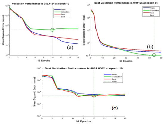
Figure 7.
The training, testing, and validation of ANN (a,b) and nonlinear autoregressive with external (exogenous) input (NARX) (c) models.
The problem of nonlinear relation minimization was solved by the Levenberg-Marquardt (LM) algorithm. The algorithm of steepest descent is known as the error backpropagation (EBP) algorithm and is considered one of the most crucial parts in the implementation of training the machine learning algorithm. However, this algorithm’s disadvantage is the slow convergence, which can be significantly enhanced by applying the Gauss-Newton algorithm. In evaluating the error surface’s curvature, it is customary to use the second-order derivatives of the error function. The Gauss-Newton algorithm can be employed for obtaining the suitable step sizes for each direction and rapidly reach convergence. As seen in Figure 7a, the error function seems to have a quadratic surface. In the initial iteration, the learning is weak (see Figure 7a), and the error rate is high. After some iterations (see Figure 7b), the algorithm could converge quickly and directly. Hence, the learning level is now high, and the error rate is low. The LM algorithm integrates two minimization methods: The steepest descent method and the Gauss-Newton algorithm, for fitting the error curve. However, combining these two algorithms reduces the variance by simultaneously updating the parameters in the steepest descent direction [49]. On the other hand, Figure 7c shows that any overfitting has occurred for the NARX with a neural network, and the training and validation errors decreased until the highlighted epoch. This approach showed an amazing performance over the others.
3.1. Levenberg–Marquardt (LM) Algorithm
As the Jacobian matrix JTJ is an invertible matrix and can be used for multilayer network training, it is expressed in the standard back propagation algorithm, and the terms in the Jacobian matrix are calculated using the LM algorithm to present the other approximation of the Hessian matrix (H) as presented in Equation (6).
where is an always positive combination coefficient, and ‘I’ is the identity matrix in Equation (6), in which the elements of the Hessian matrix are greater than zero and is always invertible. The Hessian matrix appearing in Equation (6) is updated and presented in Equation (7).
As the LM algorithm integrates the steepest descent and the Gauss-Newton algorithms, it switches between the two algorithms during the training process and gains both advantages. Where denotes the weight vector for node k, and ek is the training error of the machine learning algorithm. ‘Jk’ is the Jacobian matrix, while ‘JT’ is the transpose of m × n Jacobian matrix [49]. Selecting a very small (nearly zero) combination coefficient Equation (7) is updated and the Gauss-Newton algorithm is employed to implement the LM algorithm for the training of data obtained from the set of input parameters including x1: sulfur dioxide (SO2), x2: carbon monoxide (CO), x3: hydrogen sulfide (H2S), x4: ozone (O3), x5: nitrogen oxide (NOx), and x6: particulate matters (PM10), and the output parameters if ‘AQI.’
As seen in Figure 8, with ANNs, two problems must be solved: the calculation of the Jacobian matrix, and the organization of the training process. Considering the neuron ‘n’ with ni inputs in the first layer, all its independent parameters are connected to the network’s input layer. Equation (8) was employed to calculate the air quality index given in the neuron ‘n’ as the output of the ANN.
where fn is the activation function of neuron n and the net value ‘netn’ is the sum of weighted input nodes of neuron n which can be presented by Equation (9).
where, yn,i is the ith input node of neuron n, weighted by wn,i and wn,o. When the training of the data set is completed, a high value of correlation coefficient decently describes that the data are highly correlated with the fit. It also shows that these parameters are significantly correlated, meaning that a change in one parameter will affect the other parameters. The histogram in Figure 9a depicts the difference between the data values and the curve fit for ANN. The error histogram for the training, validation, and testing process of NARX with a neural network is presented in Figure 9b. These figures show that the curve-fit errors are normally distributed.
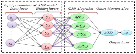
Figure 8.
The architecture of the Artificial Neural Network used for Air Quality Index Estimation.
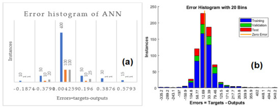
Figure 9.
Depicts the curve fit for the training, validation, and testing process of ANN (a), and NARX with neural network (b).
In this study, the redundant data were not used in the training process, as the ANN algorithm does not work well with redundant data. A multilayered perceptron (BPMLP) network with six inputs, eight processing units in the hidden layer, and one output parameter was considered for the training process. As seen in Figure 8, the back-propagation algorithms were used for training the network with LM tools’ employment, which minimizes the divergence between the input and the output parameters. The outcomes predicted by the BPMLP algorithm were converted to air quality numerals that are recorded in Table 4. During the training process, it was found that the solution had improved, as the was decreased, the LM method approached the Gauss-Newton method, and the solution usually accelerated to the local minimum [49]. Sum square error (SSE) method was employed to assess the training process. The SSE for all training patterns and network outputs was computed using Equation (10). The error rate is reasonable because redundant data and noisy data were excluded during the training, testing, and validation process. For training, 60% of data was used, 20% was used for testing, and 20% of data was used for validation. Excluding the outliers (the redundant data), the average absolute error was found at 0.07147%, and the sum of the squared errors was found at 0.0251%.
where, as seen in Equation (10), w denotes the weight vector, and ep,m refers to the training error of the machine learning algorithm.
Table 4.
AQI outputs of ANNs, ANFIS, and NARX models for certain parameters.
When using pattern p, as it is defined in Equation (11), m represents the index of outputs, from 1 to M, where M is the number of outputs.
‘d’ determines the desired output vector for air quality index (AQI), the actual output vector for AQI is represented by ‘o’. Considering the nodes and the links between the output node yj of a hidden neuron j and network output om, a complex nonlinear relationship exists between the network parameters that can be defined simply by om and , where om is the mth actual output of the network representing the air quality. Figure 10a–d depicts the targets of output for training (a), validation (b), testing (c) and all process (d) of correlation coefficient (R). The value of R is close to 1 for training, and 0.91227 for validation of data. Similarly, the value of R for testing is 0.97948 and 0.98103 for validation. The training process was initiated as shown in Figure 7a, and the final training was carried out after several training steps and illustrated in Figure 7b. The training, testing, and validation were converged at the three epochs with the validation performance of 92.3206. Thus, the result is acceptable since the final mean-square error and the absolute mean square errors are small, after several training steps, the error rates fell to 0.611236% and 0.080739%, respectively. It is also clear that the set errors of the training and testing have similar characteristics. For instance, no significant over-fitting has been obtained by iteration number thirteen, where the highest performance of the validation has occurred.
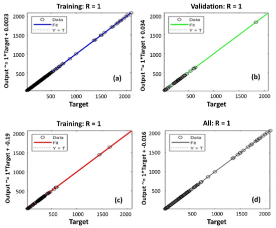
Figure 10.
Depicts the targets of output for training (a), validation (b), testing (c) and all process (d) of correlation coefficient (R).
Figure 11a and b show the histogram of error distribution and the residual is shown in c for initial and final training stages of the machine learning approach, respectively.
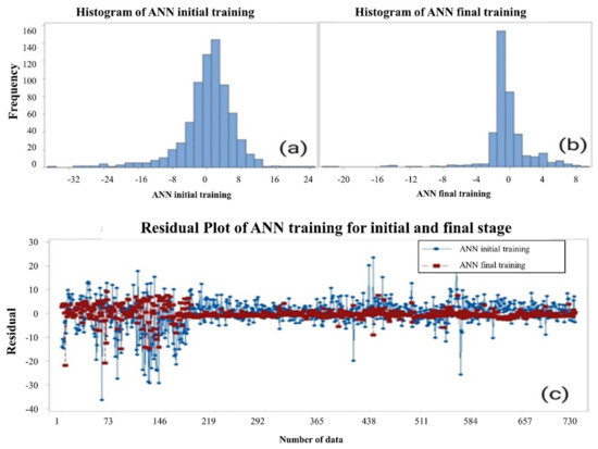
Figure 11.
(a) and (b) show the histogram of error distribution and (c) shows the residual for initial and final training stages of the machine learning approach.
3.2. Nonlinear Autoregressive with External (Exogenous) Input (NARX)
In the time-series problems, it is desired to predict future values of a time-series ‘y(t)’ from past values of that time series and past values of a second time-series ‘x(t)’. This prediction approach is labeled NARX, and can be presented as given in Equation (12):
y(t) = f(y(t − 1), …, y(t − n), x(t − 1), …, (t − n))
The standard NARX network was employed in this study which has a two-layer feedforward ANN, with a sigmoid transfer function in the hidden layer and a linear transfer function in the output layer. ‘y(t)’, the output of the NARX network, is fed back to the input of the network, because ‘y(t)’ is a function of y(t − 1), y(t − 2), …, y(t − n). where ‘t’ is the time, and ‘n’ is the amount of data. NARX can be employed to predict future values of air quality, chemical processes, manufacturing systems, robotics, and aerospace vehicles based on several variables. It can also be used for system identification, in which models are developed to represent the dynamic behavior of systems. The outputs of the training, validation, and testing process of ANNs are presented in Figure 12a. Figure 12b plots the root mean square error (RMSE) of the training, validation, and testing process of ANNs.
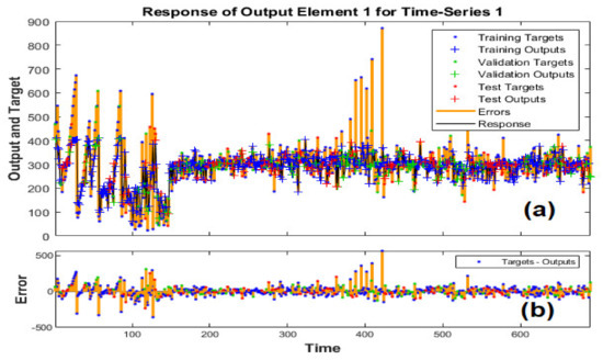
Figure 12.
(a) shows the outputs of the training, validation, and testing process of NARX with a neural network, while figure (b) plots the root mean square error (RMSE).
Figure 13 displays the error autocorrelation function. It describes how the prediction errors are related in time. For the NARX with a neural network AQI prediction model, there is one nonzero value of the autocorrelation function, and it occurred at zero lag. This is the mean square error (MSE). In the case of AQI prediction, the correlations, except for the one at zero lag, fall approximately within the 95% confidence limits around zero, so the model seems to be adequate.
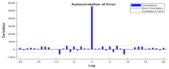
Figure 13.
The error autocorrelation function for AQI prediction.
The training, testing, and validation of the ANFIS model were converged at the 60 epochs with the validation performance of 99.3206. The mean-square error and the absolute residual rate are small in this approach; after training, they fall to 0.611236% and 0.080739%, respectively. The errors of training and testing have similar characteristics. The low-level errors obtained were due to mainly insignificancy of over-fitting observed and occurred by iteration thirteen, where the best validation performance has been observed.
The NARX with neural network showed much better performance for the same data set of independent regressors’ used for the ANN and ANFIS models. Hence, the prediction performance of NARX with the neural network approach is higher, as seen in Figure 12a,b. The NARX model training, testing, and validation were converged at the 16 epochs (see Figure 7c) with the validation performance of 99. In this approach, the mean-square error and the absolute residual rate are smaller; after training, they were determined 0.334% and 0.0475%, respectively.
4. Results and Discussion
NARX with a neural network, ANFIS, and machine learning are highly interrelated soft computing systems for information processing approaches, and capable of deep learning. They were employed for the big-data advancement of the environmental systems, using the BPMLP, two-layer feedforward ANN algorithm and steepest descent approach to reduce the mean square error of the big data set of training. The Levenberg-Marquardt (LM) [49] approach was employed as an optimization method for ANNs, as a sub-technic of machine learning approach to solve the pollutant parameters that have nonlinear relations. The results obtained were evaluated by fuzzy quality charts and compared with the US-EPA air quality standards statistically.
One of the most critical ecological issues is environmental pollution, including air, water, land pollution, etc. Emissions of sulfur dioxide and other pollutants are gradually rising as the number of industries grows [50]. Nitrogen oxides have been increasing in many locations. The widest spread of air pollution in these areas is mainly formed by the emissions created from domestic industrial plants and transportation sources. Daily arithmetic averages of sulfur dioxide, carbon-monoxide, hydrogen sulfite, ground-level ozone, nitrogen oxide, and particulate matter were collected from stations and used to model the air quality index.
Data accumulated over the last three years offered us a big data set which was substantial for training the model to obtain an ANFIS model. The AQI of each pollutant was calculated by Equation (1) and an air quality index was obtained for the cumulative effects of pollutants. Some gases are inert (like CO) and do not interact chemically with others. However, we consider the relations statistically and mathematically. This data set was then employed to train the NARX with a neural network, ANFIS, and ANN models to predict pollutants’ air quality index. The degree level of inter-correlations between the pollutants shows that atmospheric pollution depends on various parameters, the relation of some pollutants with AQI is given in Figure 14.
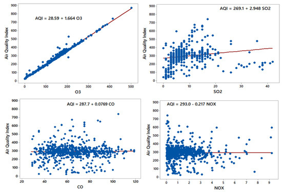
Figure 14.
The association between O3, SO2, CO, and NOx with AQI.
Ozone [51] also has a negative correlation with AQI. There is a positive correlation between O3, SO2, CO, NOx, and AQI. The associations between different air pollutants slightly vary in other relevant research that could be interpreted due to variations of different characteristics, such as location and unique meteorological factors. Table 5 shows the correlation matrix and multicollinearity between the pollutant parameters and their ‘p’ values. As the ‘p’ values are less than 0.05, they are statistically significant.
Table 5.
Correlation and multicollinearity between the parameters and p-values.
Sometimes, the forecast errors are computed in terms of percentages rather than amounts. Hence, in this study, the mean absolute percentage error (MAPE) was computed by finding the absolute error in each period, dividing this by the actual observed value for that period, and averaging these absolute percentage errors. The MAPE is a percentage and has no measurement units employed to calculate the accuracy of the same or different techniques on two entirely different series. Equation (13) shows the MAPE calculation, and it is found at 2.3747% for the AQI in this study.
On the other hand, the mean percentage error (MPE) was used to compute finding the error in each period. It is computed by finding the actual residual value for each period, then dividing by the actual AQI values to obtain the % error, and at the end, averaging these percentage errors. The MPE is calculated by Equation (14) and was found at 0.3423% for this study, which is close to zero.
As a result, when a MAPE of 2.3747% is compared to the RMSE of 5.64, the MAPE can be used to forecast the air quality data. A small MPE of 0.3423% reveals that the technique is not biased, while the value is close to zero, the techniques do not consistently over/or underestimate the AQI daily. The actual AQI observations versus the outcomes of ANN and ANFIS modeling approaches are given in Figure 15. The results clearly show that the outcomes of both models are close to the actual AQI values and the air quality is good and moderate in Jeddah. There are some deviations during some periods and this might be because of dust storms and particulate matters.
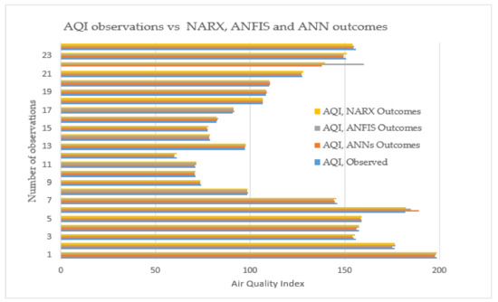
Figure 15.
Air quality index observed vs. the outcomes of NARX, ANN, and ANFIS approaches.
The NARX with a neural network, ANNs, and ANFIS model aims to construct an online and intelligent control strategy for air quality prediction. All methods produced vigorous outcomes. Table 4 illustrates NARX, ANN, and ANFIS models’ outcomes for certain pollutants versus observed air quality index. The average error was determined at 0.00335, 0.10858, and 0.10362 for NARX, ANFIS, and ANN models, respectively. On the other hand, the optimal number of rules was found to be six for the data set available for the ANFIS model. Moreover, the essential findings depicted that an additional number of membership functions and rules did not improve the ANFIS model’s efficiency [52]. Therefore, as it is given in Figure 4, six rules appear adequate to establish a rule-based ANFIS model for AQI prediction. Figure 5 depicts the fine-tuned MFs of pollutants; bell-shaped Gaussian MFs were employed for determining the membership degrees. The reason that the Gaussian MFs were employed is that the relations of parameters are nonlinear. Figure 6 shows the distribution of relative errors determined for training and testing of the ANFIS model developed for this study. The ANFIS model outcomes for certain degrees of pollutants were given in Table 4, which provides the comparison of AQI obtained from the ANFIS model, and the observed AQI obtained from the US-EPA standard [37]. In this article, the back-propagation multilayer perceptron (BPMLP) algorithm was employed to perform nonlinear mapping of parameters. The BPMLP algorithm used the Levenberg-Marquardt (LM) approach as an optimization method for solving a nonlinear least-squares problem. Figure 7a,b show the initial and final training process, respectively. Similarly, Figure 7c shows the overfitting of the NARX with neural network for training and validation error.
The training process was successfully carried out because the mean-square error and the absolute mean square errors were low and were 0.611236% and 0.080739%, respectively. Similarly, Figure 10a–d shows the training correlation coefficient (R) (a), validation R (b) and testing R (c); the R is 1 for training, validation, and testing. ANN has a similar capability for the same data set of independent regressors’ used for the ANFIS model training process. The low-level errors obtained were mainly because there was no significant over-fitting observed during iteration thirteen, where the best validation performance had been observed. Figure 11a,b show the histogram of error distribution and the residual (c) of initial and final training stages of ANN, respectively. Convergence was observed between the three parameters; hence the training process was ended.
Because of the lack of identification of the cumulative effect of quality parameters in pollution issues, a novel trend has been inspired by combining randomness and fuzziness in evaluating the environmental quality problem of air pollution in this work. Quality assessment in fuzzy sets expresses that the quality level of air is measured by membership degrees. The scatter plot of 100 principal component outcomes of AQI obtained for ANN, ANFIS and NARX models are illustrated in Figure 16 a–c, respectively.
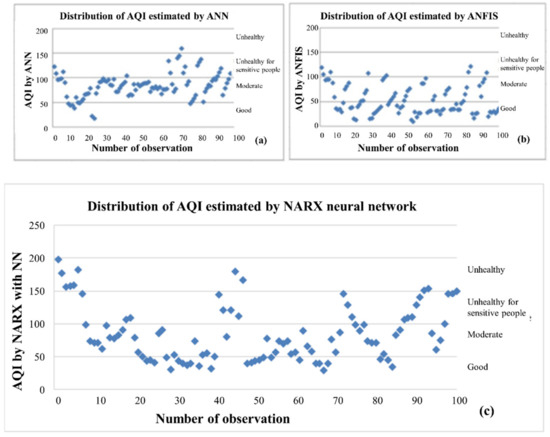
Figure 16.
The fuzzy quality assessment of AQI by ANN (a), ANFIS (b) and NARX (c) models.
Figure 16a–c shows the fuzzy quality assessment of the AQI by ANN (a), ANFIS (b), and NARX (c) models with numerical values, respectively. The fuzzy quality charts with linguistic terms were employed along with the US environmental protection agency categories for air quality index (AQI) to evaluate the air quality in Jeddah. The ANFIS and ANN are more reliable and practical approaches to observe the air quality online, which add more flexibility than the crisp assessment of air quality offline. For an overall quality assessment, when the AQI is between 0 and 50, it is defined as good air quality, if it is between 51 to 100, the air quality is moderate. However, if it is above 100, the quality is poor and unhealthy; the sensitive groups are affected. Higher AQI creates hazards (if it is above 300), which affects people’s respiratory systems. EPA [37] standards for air quality have been established to prevent several harmful effects of pollutants.
5. Conclusions
The prominent prediction techniques fall into two broad categories, namely, soft computing and statistical techniques. ARIMA (also known Box-Jenkins) and the other traditional techniques are commonly regarded as the most efficient forecasting technique in social science and are utilized broadly for time series [53]. This study aims to envisage air quality and its distribution using soft computing techniques, such as adaptive neuro-fuzzy system (ANFIS), and NARX with neural network and ANNs as machine learning approaches. The proposed methods in this work are practical, robust, and capable of estimating pollutants’ cumulative effect inside the urban areas to reduce respiratory and cardiovascular mortalities. The findings showed the remarkable performance of NARX, ANFIS, and ANN-based air quality models for high-dimensional data assessment. As a statistical approach, the usage limitation of ARIMA for forecasting time-series is crucial with uncertainty as it does not undertake knowledge of any fundamental model or input parameters as in soft computing methods [54]. The conventional techniques for the prediction of time-series, such as ARIMA, SARIMA, and many others assume that the time-series are generated from linear processes, therefore the outcomes may be inappropriate for most nonlinear real-world problems [55]. On the contrary, soft computing techniques are data-driven, self-adaptive intelligent approaches used for prediction with the ability to make generalized observations from the results obtained from original data. Additionally, machine learning approaches are universal approximators as an ANN can effectively approximate a continuous function to the anticipated accuracy level [53]. Although the literature depicts the different views on the relative superiority and performance of ANNs and ARIMA approaches for prediction, further studies are needed for a unified coherent view on these methodologies for better applications.
For the situation where the AQI values increase, people may encounter several symptoms of health concerns [37]. Air quality models’ outcomes were found meaningful for warning the public earlier in case an unhealthy situation is encountered. Air pollution management involves capacity building, monitoring ground-based networks and systems for appropriate strategic and operational decision-making. Implementing these strategies requires quality controlling and assurance, modeling approaches, and institutional capabilities. Therefore, local and global environmental policymakers can consider the presented methodologies and findings as a suitable, reliable, and useful technique in air quality assessment and management. Consequently, the stability of air quality was correlated with the absolute air quality index using soft computing techniques.
Author Contributions
The individual contribution of the authors was as follows: O.T., A.S.A., M.B. and H.A. together designed research, provide extensive advice throughout the study reading to research designed, research methodology, data collection, assessment of the results and findings and revise the manuscript. A.B., M.A. (Mohammed Alamoud), M.A. (Murad Andejany). All authors have read and agreed to the published version of the manuscript.
Funding
This work was funded by the Deanship of Scientific Research (DSR), King Abdulaziz University, Jeddah, under grant No. (RG-25-135-42).
Institutional Review Board Statement
Not applicable.
Informed Consent Statement
Not applicable.
Data Availability Statement
The data that support the findings of this study are openly available as mentioned in the reference section.
Acknowledgments
This work was funded by the Deanship of Scientific Research (DSR), King Abdulaziz University, Jeddah, under grant No. (RG-25-135-42). The authors, therefore, gratefully acknowledge the DSR technical and financial support.
Conflicts of Interest
The authors declare that they have no competing interests.
References
- Zhu, J.; Wu, P.; Chen, H.; Zhou, L.; Tao, Z.; Zhu, J.; Wu, P.; Chen, H.; Zhou, L.; Tao, Z. A Hybrid Forecasting Approach to Air Quality Time Series Based on Endpoint Condition and Combined Forecasting Model. Int. J. Environ. Res. Public Health 2018, 15, 1941. [Google Scholar] [CrossRef]
- Asadi, S.; Shahrabi, J.; Abbaszadeh, P.; Tabanmehr, S. A new hybrid artificial neural networks for rainfall-runoff process modeling. Neurocomputing 2013, 121, 470–480. [Google Scholar] [CrossRef]
- Sozzi, R.; Bolignano, A.; Ceradini, S.; Morelli, M.; Petenko, I.; Argentini, S. Quality control and gap-filling of PM10 daily mean concentrations with the best linear unbiased estimator. Environ. Monit. Assess. 2017, 189, 562. [Google Scholar] [CrossRef] [PubMed]
- Reikard, G. Volcanic emissions and air pollution: Forecasts from time series models. Atmos. Environ. 2019, 1, 100001. [Google Scholar] [CrossRef]
- Suhermi, N.; Suhartono, D.; Prastyo, D.; Ali, B. Roll motion prediction using a hybrid deep learning and ARIMA model. Procedia Comput. Sci. 2018, 144, 251–258. [Google Scholar] [CrossRef]
- Silibello, C.; D’Allura, A.; Finardi, S.; Bolignano, A.; Sozzi, R. Application of bias adjustment techniques to improve air quality forecasts. Atmos. Pollut. Res. 2015, 6, 928–938. [Google Scholar] [CrossRef]
- Donnelly, A.; Misstear, B.; Broderick, B. Real-time air quality forecasting using integrated parametric and non-parametric regression techniques. Atmos. Environ. 2015, 103, 53–65. [Google Scholar] [CrossRef]
- Rybarczyk, Y.; Zalakeviciute, R.; Rybarczyk, Y.; Zalakeviciute, R. Machine Learning Approaches for Outdoor Air Quality Modelling: A Systematic Review. Appl. Sci. 2018, 8, 2570. [Google Scholar] [CrossRef]
- Caraka, R.E.; Chen, R.C.; Yasin, H.; Lee, Y.; Pardamean, B. Hybrid Vector Autoregression Feedforward Neural Network with Genetic Algorithm Model for Forecasting Space-Time Pollution Data. Indones. J. Sci. Technol. 2021, 6, 243–266. [Google Scholar]
- Aggarwal, A.; Toshniwal, D. Detection of anomalous nitrogen dioxide (NO2) concentration in urban air of India using proximity and clustering methods. J. Air Waste Manag. 2019, 69, 805–822. [Google Scholar] [CrossRef]
- Bai, X.X.; Dong, J.; Rui, X.G.; Wang, H.F.; Yin, W.J. International Business Machines Corp. Very Short-Term Air Pollution Forecasting. U.S. Patent Application 14/939,522, 8 October 2019. [Google Scholar]
- Christin, S.; Hervet, É.; Lecomte, N. Applications for deep learning in ecology. Methods Ecol. Evol. 2019, 10, 1632–1644. [Google Scholar] [CrossRef]
- Fairbrass, A.J.; Firman, M.; Williams, C.; Brostow, G.J.; Titheridge, H.; Jones, K.E. CityNet—Deep learning tools for urban ecoacoustic assessment. Methods Ecol. Evol. 2019, 10, 186–197. [Google Scholar] [CrossRef]
- Torney, C.J.; Lloyd-Jones, D.J.; Chevallier, M.; Moyer, D.C.; Maliti, H.T.; Mwita, M.; Kohi, E.M.; Hopcraft, G.C. A comparison of deep learning and citizen science techniques for counting wildlife in aerial survey images. Methods Ecol. Evol. 2019, 10, 779–787. [Google Scholar] [CrossRef]
- Sayeed, A.; Choi, Y.; Eslami, E.; Lops, Y.; Roy, A.; Jung, J. Using a deep convolutional neural network to predict 2017 ozone concentrations, 24 hours in advance. Neural Netw. 2019, 121, 396–408. [Google Scholar] [CrossRef]
- Munawar, S.; Hamid, D.; Khan, M.S.; Ahmed, A.; Hameed, N. Health Monitoring Considering Air Quality Index Prediction Using Neuro-Fuzzy Inference Model: A Case Study of Lahore, Pakistan. J. Basic Appl. 2017, 12, 123–132. [Google Scholar] [CrossRef]
- Rahman, M.M.; Shafiullah, M.; Rahman, S.M.; Khondaker, A.N.; Amao, A.; Zahir, M. Soft Computing Applications in Air Quality Modeling: Past, Present, and Future. Sustainability 2020, 12, 4045. [Google Scholar] [CrossRef]
- Hvidtfeldt, U.A.; Sorensen, M.; Geels, C.; Ketzel, M.; Khan, J.; Tjonneland, A.; Overvad, K.; Brandt, J.; Raaschou-Nielsen, O. Long-term residential exposure to PM2.5, PM10, black carbon, NO2, and ozone and mortality in a Danish cohort. Environ. Int. 2019, 123, 265–272. [Google Scholar] [CrossRef]
- Ansari, M.; Ehrampoush, M.H. Meteorological correlates and AirQ+ health risk assessment of ambient fine particulate matter in Tehran, Iran. Environ. Res. 2019, 170, 141–150. [Google Scholar] [CrossRef]
- Liu, F.; Chen, G.; Huo, W.; Wang, C.; Liu, S.; Li, N.; Mao, S.; Hou, Y.; Lu, Y.; Xiang, H. Associations between long-term exposure to ambient air pollution and risk of type 2 diabetes mellitus: A systematic review and meta-analysis. Environ. Pollut. 2019, 252, 1235–1245. [Google Scholar] [CrossRef]
- Alimissis, A.; Philippopoulos, K.; Tzanis, C.G.; Deligiorgi, D. Spatial estimation of urban air pollution with the use of artificial neural network models. Atmos. Environ. 2018, 191, 205–213. [Google Scholar] [CrossRef]
- Cabaneros, S.M.; Calautit, J.K.; Hughes, B.R. A review of artificial neural network models for ambient air pollution prediction. Environ. Model. Softw. 2019, 119, 285–304. [Google Scholar] [CrossRef]
- Taylan, O. Modelling and analysis of ozone concentration by artificial intelligent techniques for estimating air quality. Atmos. Environ. 2017, 150, 356–365. [Google Scholar] [CrossRef]
- Pawlak, I.; Jarosławski, J.; Pawlak, I.; Jarosławski, J. Forecasting of Surface Ozone Concentration by Using Artificial Neural Networks in Rural and Urban Areas in Central Poland. Atmosphere 2019, 10, 52. [Google Scholar] [CrossRef]
- Biancofiore, F.; Busilacchio, M.; Verdecchia, M.; Tomassetti, B.; Aruffo, E.; Bianco, S.; Di Tommaso, S.; Colangeli, C.; Rosatelli, G.; Di Carlo, P. Recursive neural network model for analysis and forecast of PM10 and PM2.5. Atmos. Pollut. Res. 2017, 8, 652–659. [Google Scholar] [CrossRef]
- Telesca, V.; Caniani, D.; Calace, S.; Marotta, L.; Mancini, I.M. Daily temperature and precipitation prediction using neuro-fuzzy networks and weather generators. In Proceedings of the International Conference on Computational Science and Its Applications, Trieste, Italy, 3–6 July 2017. [Google Scholar]
- Caraka, R.E.; Chen, R.C.; Yasin, H.; Pardamean, B.; Toharudin, T.; Wu, S.H. Prediction of Status Particulate Matter 2.5 using State Markov Chain Stochastic Process and Hybrid VAR-NN-PSO. IEEE Access 2019, 7, 161654–161665. [Google Scholar] [CrossRef]
- Grivas, G.; Chaloulakou, A. Artificial neural network models for prediction of PM10 hourly concentrations, in the Greater Area of Athens, Greece. Atmos. Environ. 2006, 40, 1216–1229. [Google Scholar] [CrossRef]
- Jorquera, H.; Perez, R.; Cipriano, A.; Espejo, A.; Victoria Letelier, M.; Acuna, G. Forecasting ozone daily maximum levels at Santiago, Chile. Atmos. Environ. 1998, 32, 3415–3424. [Google Scholar] [CrossRef]
- Ghoneim, O.A.; Manjunatha, B.R. Forecasting of ozone concentration in the smart city using deep learning. In Proceedings of the 2017 International Conference on Advances in Computing, Communications, and Informatics, ICACCI 2017, Udupi, India, 13–16 September 2017; Institute of Electrical and Electronics Engineers Inc.: Piscataway, NJ, USA, 2017; pp. 1320–1326. [Google Scholar]
- Zhou, Y.; Chang, F.J.; Chang, L.C.; Kao, I.F.; Wang, Y.S. Explore a deep learning multi-output neural network for regional multi-step-ahead air quality forecasts. J. Clean. Prod. 2019, 209, 134–145. [Google Scholar] [CrossRef]
- Ayturan, Y.A.; Ayturan, Z.C.; Altun, H.O. Air pollution modeling with deep learning: A review. Int. J. Environ. Pollut. Environ. Model. 2018, 1, 58–62. [Google Scholar]
- Zhou, K.; Xie, R. Review of neural network models for air quality prediction. In International Conference on Big Data Analytics for Cyber-Physical-Systems; Springer: Berlin/Heidelberg, Germany, 2020; Volume 1117, pp. 83–90. [Google Scholar]
- Iskandaryan, D.; Ramos, F.; Trilles, S. Air Quality Prediction in Smart Cities Using Machine Learning Technologies based on Sensor Data: A Review. Appl. Sci. 2020, 10, 2401. [Google Scholar] [CrossRef]
- Sowlat, M.H.; Gharibi, H.; Yunesian, M.; Mahmoudi, M.T.; Lotfi, S. A novel, Fuzzy-based air quality index (FAQI) for air quality assessment. Atmos. Environ. 2011, 45, 2050–2059. [Google Scholar] [CrossRef]
- EPA. Guideline on Air Quality Models (Revised); 40 CFR 51; US EPA: Washington, DC, USA, 2005. [Google Scholar]
- US EPA. Guideline for Developing an Ozone Forecasting Program; EPA-454/R-99-009; US EPA: Washington, DC, USA, 1999. [Google Scholar]
- Kaur, G.; Gao, J.; Chiao, S.; Lu, S. Air Quality Prediction: Big data and Machine Learning Approaches. In Proceedings of the 5th International Conference on Sustainable Environment and Agriculture (ICSEA 2017), Los Angeles, CA, USA, 28–30 October 2017. [Google Scholar]
- Masmoudi, S.; Elghazel, H.; Taieb, D.; Yazar, O.; Kallel, A. A machine-learning framework for predicting multiple air pollutants’ concentrations via multi-target regression and feature selection. Sci. Total Environ. 2020, 715, 136991. [Google Scholar] [CrossRef] [PubMed]
- Maciąg, P.S.; Kasabov, N.; Kryszkiewicz, M.; Bembenik, R. Air pollution prediction with clustering-based ensemble of evolving spiking neural networks and a case study for London area. Environ. Model Softw. 2019, 118, 262–280. [Google Scholar] [CrossRef]
- Pan, S.; Choi, Y.; Roy, A.; Jeon, W. Allocating emissions to 4 km and 1 km horizontal spatial resolutions and its impact on simulated NOx and O3 in Houston, TX. Atmos. Environ. 2017, 164, 398–415. [Google Scholar] [CrossRef]
- Wang, D.; Wei, S.; Luo, H.; Yue, C.; Grunder, O. A novel hybrid model for air quality index forecasting based on two-phase decomposition technique and modified extreme learning machine. Sci. Total Environ. 2017, 580, 719–733. [Google Scholar] [CrossRef]
- Prasad, K.; Gorai, A.K.; Goyal, P. Development of ANFIS models for air quality forecasting and input optimization for reducing the computational cost and time. Atmos. Environ. 2016, 128, 246–262. [Google Scholar] [CrossRef]
- Ishibuchi, H.; Nakashima, T.; Murata, T. Performance evaluation of fuzzy classifier systems for multidimensional pattern classification problems. IEEE Trans. Syst. Man Cybern. Part B Cybern. 1999, 29, 601–618. [Google Scholar] [CrossRef]
- El Raey, M. Air Quality and Atmospheric Pollution in the Arab Region, Economic and Social League of Arab States, Commission for Western Asia Joint Technical Secretariat of the Council of Arab Ministers Responsible for the Environment; University of Alexandria: Alexandria, Egypt, 2006. [Google Scholar]
- Taylan, O.; Karagozoglu, B. An Adaptive Neuro-fuzzy model for prediction of student’s academic performance. J. Comput. Ind. Eng. 2009, 57, 732–741. [Google Scholar] [CrossRef]
- Al-Alawi, S.M.; Abdul-Wahab, S.A.; Bakheit, C.S. Combining principal component regression and artificial neural networks for more accurate predictions of ground-level ozone. Environ. Model Softw. 2008, 23, 396–403. [Google Scholar] [CrossRef]
- Jang, J.S.R.; Sun, C.T.; Mizutani, E. Neuro-Fuzzy and Soft Computing; Prentice-Hall: Hoboken, NJ, USA, 1997. [Google Scholar]
- Wilamowski, B.M.; Yu, H. Improved Computation for Levenberg Marquardt Training. IEEE Trans. Neural Netw. 2010, 21, 930–937. [Google Scholar] [CrossRef]
- Wahab, S.A. The role of meteorology on predicting SO2 concentrations around a refinery: A case study from Oman. Ecol. Model. 2006, 197, 13–20. [Google Scholar] [CrossRef]
- Wahab, A.S.; Bakheit, S.C.; Al-Alawi, S. Principal component and multiple regression analysis in modeling of ground-level ozone and factors affecting its concentrations. Environ. Model Softw. 2005, 20, 1263–1271. [Google Scholar] [CrossRef]
- Taylan, O. Estimating the quality of process yield by fuzzy sets and systems. Expert Syst. Appl. 2011, 38, 12599–12607. [Google Scholar] [CrossRef]
- Adebiyi, A.A.; Adewumi, A.O.; Ayo, C.K. Comparison of ARIMA and Artificial Neural Networks Models for Stock Price Prediction. J. Appl. Math. 2014, 2014, 614342. [Google Scholar] [CrossRef]
- Zhang, G.; Patuwo, B.; Hu, M.Y. Forecasting with artificial neural networks: The state of the art. Int. J. Forecast. 1998, 14, 35–62. [Google Scholar] [CrossRef]
- Khashei, M.; Bijari, M.; Ardali, G.A.R. Improvement of auto-regressive integrated moving average models using fuzzy logic and artificial neural networks (ANNs). Neurocomputing 2009, 72, 956–967. [Google Scholar] [CrossRef]


Publisher’s Note: MDPI stays neutral with regard to jurisdictional claims in published maps and institutional affiliations. |
© 2021 by the authors. Licensee MDPI, Basel, Switzerland. This article is an open access article distributed under the terms and conditions of the Creative Commons Attribution (CC BY) license (https://creativecommons.org/licenses/by/4.0/).