Article

The Temporal and Spatial Changes of Ship-Contributed PM2.5 Due to the Inter-Annual Meteorological Variation in Yangtze River Delta, China

1
Key Laboratory of Beijing on Regional Air Pollution Control, Beijing University of Technology, Beijing 100124, China
2
Institute of Technical Information for Building Materials Industry of China, Beijing 100024, China
*
Authors to whom correspondence should be addressed.
Atmosphere 2021, 12(6), 722; https://doi.org/10.3390/atmos12060722
Submission received: 26 April 2021 / Revised: 27 May 2021 / Accepted: 31 May 2021 / Published: 4 June 2021
(This article belongs to the Section Air Quality)

Abstract

:
Ship-exhausted air pollutants could cause negative impacts on air quality, climate change, and human health. Increasing attention has been paid to investigate the impact of ship emissions on air quality. However, the conclusions are often based on a specific year, the extent to which the inter-annual variation in meteorological conditions affects the contribution is not yet fully addressed. Therefore, in this study, the Weather Research and Forecast model and the Community Multiscale Air Quality model(WRF/CMAQ) were employed to investigate the inter-annual variations in ship-contributed PM2.5 from 2010 to 2019. The Yangtze River Delta (YRD) region in China was selected as the target study area. To highlight the impact of inter-annual meteorological variations, the emission inventory and model configurations were kept the same for the 10-year simulation. We found that: (1) inter-annual meteorological variation had an evident impact on the ship-contributed PM2.5 in most coastal cities around YRD. Taking Shanghai as an example, the contribution varied between 3.05 and 5.74 µg/m3, with the fluctuation rate of ~65%; (2) the inter-annual changes in ship’s contribution showed a trend of almost simultaneous increase and decrease for most cities, which indicates that the impact of inter-annual meteorological variation was more regional than local; (3) the inter-annual changes in the northern part of YRD were significantly higher than those in the south; (4) the most significant inter-annual changes were found in summer, followed by spring, fall and winter.

1. Introduction

As one of the most important components in international trade, the global seaborne trade has continued to grow in the past decades [1,2]. In 2019, the total volumes exceeded 11 billion tons, accounting for more than 80% of world trade [3]. The booming ship transportation caused a large amount of energy consumption and air pollutant emissions [3,4,5,6,7,8,9]. Those exhausted air pollutants, which include sulfur oxides (SOx), nitrogen oxides (NOx), particulate matters (PM) and hydrocarbons (HC), could cause negative impacts on air quality, climate change, and human health [10,11,12,13,14,15,16]. Jonson et al. (2020) [17] reported that shipping is responsible for 10% or more of the controllable particles with an aerodynamic diameter of 2.5 µm or less (PM2.5) concentrations in coastal countries. Study in Europe [18] found that the annual mean contribution of ship emissions to PM2.5 in coastal cities varied between 1 and 14%. Studies have shown that nearly 70% of ship emissions are generated within 400 km of land [11,19], and these emissions not only have a significant impact near the shore, but also extend to inland areas due to the long-distance transportation of air pollutants over several hundreds of kilometers [12]. People living in coastal cities are more vulnerable to greater health risks and more severe negative impacts from shipping pollution [20,21]. In East Asia, it is estimated that 14,500–37,500 premature deaths per year could be attributed to exposure to shipping emissions [12].
In line with Asian economies’ strong contribution to global trade, Asia is by far the largest seaborne trading region. In 2019, 62% of all goods were unloaded and over 40% of all goods were loaded in Asian seaports [22]. Among Asian countries, the economy best connected to the global liner shipping network was China, and the rank order remained almost unchanged over the last ten years. As the economic center of China and one of the busiest port clusters in the world, the Yangtze River Delta (YRD) region in China has many large ports, with Shanghai Port and Ningbo-Zhoushan Port rank the first and fourth of the top ten container ports in the world, respectively [23].
Numerous studies have investigated the impact of ship emissions on air quality in YRD region. However, their conclusions are often based on a specific year [24,25,26,27,28,29,30,31,32,33,34], and whether the meteorological conditions are typical enough to represent the normal meteorological conditions of the study area is often neglected. Consequently, many of these studies have conflicting results. For example, Chen et al. (2019) [33] used the Weather Research and Forecast (WRF) model and the Community Multiscale Air Quality (CMAQ) model to quantify the impact of ships on PM2.5 in the YRD region, the results show that the annual average contribution of ship emissions to PM2.5 is 2.1 μg/m3 in 2014. However, Feng et al. (2019) [34] employed the same model and found that ships contributed only 0.56 μg/m3 to the ambient PM2.5 concentrations across the YRD in 2015. When faced with these conflicting results, it is difficult for policymakers to set a scientific basis for control measures and strategies.
There are many reasons for these differences, including the different selection of representative months for annual average calculation, the inter-annual variation in pollutant emissions, the different configurations of modeling systems, and the inter-annual variation in meteorological conditions. Among these influencing factors, meteorology may play a role that cannot be neglected. Previous studies have revealed that there was a large meteorologically driven inter-annual variability in PM2.5 [35], the impact of inter-annual meteorological conditions on PM2.5 was important and showed significant spatiotemporal variations [36]. Even if emissions remain unchanged, adverse weather conditions may lead to an increase in air pollutants [37,38,39,40]. In some cases, compared with emission control, meteorological conditions even played a leading role [41], and was likely to significantly offset the emission reduction effect. However, these studies mainly focused on the inland air pollution issues, the extent to which the inter-annual variation in meteorological conditions affects the contribution of shipping emissions, which is sensitive to the variation in meteorology [42], is not yet fully addressed.
To address this knowledge gap, a comprehensive air quality modeling system (WRF/CMAQ) was employed in this study to investigate the variation in the ship’s contribution to PM2.5 from 2010 to 2019 under the same emissions scenario. The YRD region in China, which is one of the busiest port clusters in the world, was selected as the target area for the investigation. It should be noted that the model configurations were kept the same throughout our research process to highlight the change of the shipping contribution owing to the inter-annual variation of the meteorology. The results of this research will help to enhance our understanding of the variation in ship-contributed PM2.5 under various meteorological conditions that occurred in different years. Further, the results will help policymakers to formulate policies and strategies that are more effective for emission abatement and reduce the uncertainty due to the selection of a specific year.

2. Methodology

2.1. Study Area

The Yangtze River Delta region, which is made up of Shanghai Municipality and the provinces of Jiangsu, Zhejiang and Anhui, is an important international gateway and one of the busiest port clusters in the world. Among the 23 large ports in this area, the Shanghai and Ningbo-Zhoushan ports in this region are two of the busiest ports in the world, ranked first and fourth, respectively, in the 2018 container traffic world port rankings [21]. In this paper, the study area was set from 26.2° N to 35.7° N and 113.5° E to 126.4° E, covering all ports of YRD region, as shown in Figure 1.

2.2. Climate and Air Quality of the Study Area

Located on the eastern coast of China, YRD features a typical monsoon climate with four distinct seasons. The annual mean temperature from 2010 to 2019 varies between 16 °C and 18 °C, and the annual precipitation varies between 1000 mm and 1700 mm with uneven seasonal distributions: the most in summer (300~800 mm) and the least in winter (60~400 mm) [43]. The wind regimes also show strong seasonality, being affected by the western Pacific subtropical high in summer and Siberian (or Mongolian) cold high in winter, spring and autumn [44]. The southeast wind blows from the southeast sea surface in summer, and the northwest wind is prevalent in winter [45].
Monitoring data during 2010–2019 show that the overall air quality in YRD has improved greatly, the concentration of most pollutants has continuously decreased (e.g., in Shanghai, the annual average concentration of PM2.5 has dropped from 61 μg/m3 to 31 μg/m3), whereas the ozone pollution has become increasingly apparent [46,47]. The air pollution in YRD exhibits obvious seasonal changes, characterized by high particulate matter pollution in autumn and winter and high ozone pollution in summer and spring [46,47]. Previous research indicates that the air quality in YRD was affected not only by local emissions but also by regional transport of pollutants [48,49,50,51].

2.3. Model Configuration and Input Data

The WRF/CMAQ modeling system was used in this study to investigate the temporal and spatial changes of ship-contributed PM2.5 due to the inter-annual meteorological variation from 2010 to 2019. Figure 1 displays the sketch map of the study area and the two nested domains that are established for the modeling system. Domain 1 covered the whole of China and part of China’s offshore waters, with a grid resolution of 27 km × 27 km (154 rows and 180 columns). Domain 2 covered the YRD region and some surrounding areas, with a grid resolution of 9 km × 9 km (95 rows and 116 columns). January, April, July and October of each year from 2010 to 2019 were selected as the target periods of simulation, which represent winter, spring, summer and fall of the ten years, respectively. The emissions (emission inventory of 2014) and model configurations were kept the same, while the meteorological data for each year were used in the 10-year simulation to highlight the impact of inter-annual meteorological changes. All configurations of the CMAQ model were kept consistent for two scenarios except for emission inputs. Previous research indicates that the practice to “spin up” a model for a certain time prior to the study period of interest could reduce or eliminate the effects of initial conditions [52,53,54]. In this study, a spin up time of three days, which has been extensively applied and evaluated in previous studies [8,25,34,55,56,57,58,59], was used for both WRF and CMAQ model for each month.
The WRF model configuration: The Purdue Lin microphysics scheme [60], the Noah Land-Surface scheme [61], the Yonsei University (YSU) Planetary Boundary Layer (PBL) physics scheme [62], New Goddard shortwave radiation scheme [63], and the GFDL longwave radiation scheme [64] were selected as the major meteorological physical schemes of the model in this study.
The CMAQ model configuration: The Carbon Bond-05(CB05) mechanism with chlorine and update toluene chemistry [65] was used for gas-phase chemical mechanism, and the six-generation modal CMAQ aerosol mode (AERO6) with extensions for sea salt emission and thermodynamics [66,67] was used as the aerosol mechanism.
Meteorological data: The meteorological initial and boundary conditions for the WRF model were provided by «National Center for Environmental Prediction» (NCEP) FNL (Final) operational global analysis data with a horizontal resolution of 1° × 1° and a temporal resolution of 6 h [68].
Emission data: The emission data used in this study include the emissions from shipping and other anthropogenic and natural sources. The ship emission inventory for the study was established by Chen et al. [69] with a high spatiotemporal resolution in China. Based on this inventory, the total ship emissions in this study area were 4.5 × 10⁵ (SO2), 8.25 × 10⁵ (NOx), 6.3 × 10⁴ (PM2.5), 6.8 × 10⁴ (PM10), 4.2 × 10⁴ (HC), and 8.8 × 10⁴ (CO) tonnes/yr, respectively. Figure 2 shows the spatial distribution of annual shipping emissions from the YRD region in 2014. Other anthropogenic emission inventories were obtained from the Multi-resolution Emission Inventory of China (MEIC) in 2014 [70,71,72,73]. The biomass burning emission inventory developed by Zhou et al. [74] was used in this study. The emissions from natural sources were calculated by the Biogenic Emission Inventory System incorporated in the Sparse Matrix Operator Kernel Emissions model.

2.4. Model Evaluation

The WRF model and The CMAQ model have been extensively applied and evaluated in our previous studies [75,76,77,78,79,80,81,82,83] and those of other researchers [21,84,85,86,87]. Most of these studies have produced encouraging results. In this study, similar evaluating methods that have been employed by Chen et al. [33,82,83] were used. Generally, the statistical metrics used in model evaluation included correlation coefficient(R), the Average in Observations (AVG-obs), the Average in Simulations (AVG-sim), the Mean Absolute Error (MAE), the Mean Fractional Bias (MFB), the Mean Fractional Error (MFE), the Normalized Mean Bias (NMB) and the Normalized Mean Error (NME).
To evaluate the performance of the WRF model, the comparison of simulated and observed meteorological parameters (including temperature at 2 m, T2; relative humidity at 2 m, RH2; and wind speed at 10 m, WS10) for each simulated month (January, April, July, October in 2014) are shown in Table 1. The monitoring data at every 1 or 3 h (most at 3 h) from 150 meteorological stations which were located in or near the core coastal cities were obtained from the National Climate Data Center [88]. High correlation coefficients (R, 0.7–0.9) and low Mean Absolute Error (MAEs, 0.86–8.36) proved that the model performances were acceptable.
To evaluate the performance of the CMAQ model, the comparison of simulated and observed concentrations in 171 sites that are well distributed in China for each simulated month (January, April, July, October in 2014) are shown in Table 2. It is exhibited that the high correlation coefficient (from 0.70 to 0.90) between the simulated concentrations and the observed concentrations. The value of MFB and MFE ranged from −21.96% to 2.52% and from 8.77% to 26.51%, respectively, which are within the suggested criteria (MFB ± 60% and MFE < 75%) for particulate matter modeling by Boylan and Russell [89].
The results indicate that the simulated values generally agreed with the observations, but differences were also found between the simulation results and the observational data. These deviations might be explained by the inherent uncertainty of the meteorological input, emission inventory, and the unavoidable deficiencies of the meteorological and the air quality models [31].

3. Results

In this study, the impacts on PM2.5 of shipping were estimated based on modeling results of two scenarios, with and without ship emissions. The difference in simulated PM2.5 between the two scenarios was considered as the ship’s contribution. The influence of inter-annual meteorological variation on the ship-contributed PM2.5 in YRD from 2010 to 2019 was then investigated. To highlight the impact of the inter-annual meteorological changes, the emissions (emission inventory of 2014) and model configurations were kept the same, while the meteorological data for each year were used in the 10-year simulation. In the following sections, we will discuss the annual, seasonal and spatial distribution changes of ship-contributed PM2.5 due to the inter-annual meteorological variation.

3.1. Annual Changes of Ship-Contributed PM2.5

The annual mean contribution of the ship emissions to PM2.5 was extrapolated from the mean value of January, April, July and October, which represent the four seasons of winter, summer, fall and spring, respectively. It should be noted that choosing a whole year rather than only using representative months to carry out the simulation work will get more comprehensive results. As 10-year simulation is computationally intensive, choosing such a calculation scheme helps us strike a balance between efficiency and accuracy. However, the annual average calculated based on four representative months inevitably deviates from the result based on the whole year. The bias could be towards overestimating inter-annual variability in our study, because one season is the sum of three consecutive months, so a one-month period aggregates inter-annual variability and intraseasonal variability, the latter one being partly smoothed out on seasonal averages. The main modes of meteorological intraseasonal variability in the region may also enlarge the range of change. For example, in winter, due to the influence of the Northwest Siberian and Mongolian cold high, the YRD region is controlled by the north-westly wind according to the locations of high- and low-pressure systems in the YRD, and the speed of wind has obvious intraseasonal variability [90]. The comparison of some meteorological variables (including temperature at 2 m, the relative humidity at 2 m and the wind speed at 10 m) of one-month and three consecutive months in four seasons of 2014 also support this point. The results of the comparison were not placed in the text for the purpose of conciseness. The average ship-contributed PM2.5 in µg/m3 (add ship − no ship) and in % (add ship − no ship) × 100%/(add ship) from 2010 to 2019 over YRD was shown in Figure 3a,b, respectively. It was found that ship emissions caused an evident increase in PM2.5, not only in port and coastal areas but also over wider inland regions. With the increase in the distance from coastline, the ship-contributed PM2.5 gradually decreases. The results show that the 10-year average ship contribution of PM2.5 to the whole land areas in YRD region was 1.41 µg/m3 (~3.0%). It was up to 4.57 µg/m3 in coastal areas, and as the distance from the coastline increased, the contribution was reduced to less than 0.5 μg/m3 (1%) far inland. For the coastal cities, it was found that both contribution value and contribution rate varied significantly in different coastal cities (e.g., Zhoushan 4.57 μg/m3, 18% and Hangzhou 0.47 μg/m3, ~1%). The contribution rates of ship emissions in some cities are close, but the contribution values are different. For example, the contribution rates for both Taizhou and Suzhou are 6%, but the contribution values are 1.65 µg/m3 and 2.39 µg/m3, respectively. This indicates that different coastal cities need to adopt different priorities when formulating control policies for ship pollution.
In coastal areas that were significantly affected by ship emissions, the influence along the northern coastline of YRD was much more evident than the southern coastline. To understand the cause of this phenomenon, we first try to see if this difference was caused by the distribution of the intensity of ship emissions and the distance of the shipping routes from the coastline. To our surprise, this is exactly the opposite of what we expected. Comparing the spatial distribution map of ship emissions in Figure 2, it was found that the intensity of ship emissions in the offshore areas of the southern coastline was considerably greater than that in the northern coastline, and the distance from the shipping routes to the coastline in the southern coastal areas was also much closer to that in the northern coastal areas.
The 10-year average wind vectors in YRD give us a clue to explain the spatial inhomogeneity of ship’s contribution. As shown in Figure 3, the wind vectors in the coastal waters of YRD were mostly southwestward. The wind blew inland perpendicular to the northern part of YRD coastline, while the wind vectors over the southern coastline was mostly parallel to the coastline. Under the influence of such a wind field, the ship emissions in the northern coastal waters of YRD were transported more readily inland than that in the southern coastal waters. As a result, ship emissions had a more significant impact on the northern coastal area of YRD. However, it should be noted that the YRD region is subject to the East Asian monsoon regime and the wind changes sign and even direction according to seasons. Interpreting the year averaged wind has less meaning compared to the seasonal analysis, and it only reflects the average condition of the wind field in YRD to a certain extent. In the next section on seasonal analysis, we may find that although the wind in October appears to be the annual average, but the distribution of the contributed PM2.5 may be very different.
Given that coastal zones were more affected by ship emissions than inland areas, we selected 14 cities along the coastline of the YRD to study the influence of inter-annual meteorological variation on the ship-contributed PM2.5. As shown in Figure 3, the averaged increases in PM2.5 due to ship emissions in 14 coastal cities were ~7% (2.24 µg/m3). The values in cities with large ports such as Zhoushan and Shanghai are 18% (4.57 µg/m3) and 12% (4.14 µg/m3), respectively. Is was also found in Figure 3 that ship-contributed PM2.5 in most cities showed remarkable inter-annual fluctuation from 2010 to 2019. Take Shanghai as an example, ship-contributed PM2.5 varied between 3.05 and 5.74 µg/m3, with the fluctuation rate of ~65%. Note that the fluctuation rate is defined as (max − min)/average.
China’s climate is strongly affected by the Asian monsoon, especially in the YRD region. The strength of the Asian monsoon exhibits large inter-annual variations as a result of the interactions between atmosphere and oceans [91]. Pervious research indicates that meteorological fields are quite different in magnitude between strong and weak monsoon years [92,93,94,95,96,97]. In a strong summer monsoon year, there are large rainfall in northern China and a deficit of rainfall in southern China, while the situation is the opposite in a strong monsoon year [92,93,94]. The YRD region is located in the eastern part of China and is the junction area of South China and North China, so it is more affected by the inter-annual changes of the East Asian monsoon. Zhang et al. (2010) found that the surface layer PM2.5 concentration averaged over June–August over eastern China is 44.3% higher in the weak monsoon year than in the strong monsoon year by assuming same emissions in simulations for these 2 years [98]. The simulation analysis of Cheng et al. (2016) showed that amplitudes of the inter-annual variability in surface aerosols were up to 20–30% relative to the 10-year averages over eastern China, which was driven by fluctuation in meteorological factors, such as near-surface winds, precipitation and atmospheric boundary layer, associated with East Asian Monsoon changes [99]. These inter-annual variations in meteorological fields associated with the Asian monsoon could also influence the PM2.5 concentration over the YRD region by influencing the transport, chemical reactions, and deposition of aerosols.
To identify whether the ship-contributed PM2.5 in each year is higher or lower than usual due to the inter-annual meteorological variation, the contribution anomaly between each year’s value and the 10-year average was calculated (as displayed in Figure 4). The term “anomaly” refers to a departure from the reference value or long-term average. For the contribution anomalies discussed herein, the reference value is the average contribution of ship emissions over the 2010–2019 period. The red bars (positive anomaly) denote higher values than the average, and the blue bars (negative anomaly) represent lower values than the average. The longer the bar, the higher the departure from the long-term average. The shorter the bar, the closer the value is to the 10-year average.
By comparing the contribution anomalies of the 14 coastal cities over the 2010–2019 period, notable inter-annual variation was found in most coastal cities, as displayed in Figure 4. This is especially true in cities where the impact of ships s relatively more pronounced. Specifically, for cities with the annual ship-contributed PM2.5 over 3 µg/m3, such as Zhoushan, Shanghai and Nantong, the contribution anomalies ranged from −1.24 µg/m3 to 2.64 µg/m3. There were also cities where the ship’s contribution did not change significantly from year to year, such as Shaoxing and Hangzhou, with the contribution anomalies ranged from −0.31 to 0.32 µg/m3. The reason may be that these cities were located in the south of the YRD, as we have previously discussed, the average wind vectors over southern coastal waters of YRD were almost parallel to the coastline, the influence of ships was not very significant.
Another interesting finding is that the inter-annual changes in ship’s contribution show a trend of almost simultaneous increase and decrease for most cities, which indicates that the impact of inter-annual meteorological variation on the ship contribution was more regional than local. This conclusion is especially true for extreme years when the annual anomaly values were relatively high (2014, 2015 and 2018) or low (2011–2013), as shown in Figure 4.
As displayed in Figure 4, we also calculated the anomaly of all PM2.5, the grey bars and white bars represent positive anomaly and negative anomaly, respectively. By comparing the inter-annual variability of ship pollution and all PM2.5 pollution, we found that in the years with relative lower all PM2.5 (negative anomaly, for example 2011, 2012 and 2013), the inter-annual variability of ship pollution and all PM2.5 pollution followed the same patterns of variation. However, the situation becomes more complicated when the all PM2.5 pollution was significantly greater than the historical average. In 2018, for example, the inter-annual variability of ship pollution and all PM2.5 pollution followed the same variation patterns for 14 coastal cities, while only 5 out of 14 coastal cities showed the same trend in 2017. In addition, when the impact of ships was significantly higher than the historical average, for example in 2014 and 2015, the all PM2.5 pollution did not show a significant deviation and was closed to the historical average. These results indicate that only in the years with relatively lower PM2.5, the inter-annual variability of ship pollution and all PM2.5 pollution followed the same patterns of variation.

3.2. Seasonal Changes of Ship-Contributed PM2.5

Figure 5 displays the 10-year averaged ship’s contribution to PM2.5 in YRD region in the four seasonal representative months. Generally, the simulated results indicated that ship emissions caused evident increase to PM2.5 concentration in all seasons and exhibited dramatic seasonal variation. It can be seen from the figure that the ship’s impacts in spring and summer were more significant than that in fall and winter, and much sharper gradient of contributed PM2.5 was found near the coastline in spring and summer. By averaging ship’s contribution to PM2.5 in the 14 coastal cities, the results also verify this seasonal trend: with summer (3.19 μg/m3) > spring (2.33 μg/m3) > fall (1.44 μg/m3) > winter (1.00 μg/m3). The average wind direction in different seasons may be an important factor affecting the spatial distribution of ship emissions. It was found that the onshore airflow in spring and summer was more evident, and pollutants emitted by ships were more likely to be transported landward. In winter, the northly wind was almost parallel to the coastline, and the impact of ship emissions on land was the smallest in the four seasons, both in terms of space and extent. In fall, there was mainly northeast airflow in coastal areas, and the wind vectors had greater shore component in the northern coastal area of YRD, resulting in a very obvious transport of pollutants to far inland in northern YRD. Due to the relatively high wind speed and consistent wind direction, the contributed PM2.5 was more evenly distributed with relatively lower concentration, but the impact range (the penetration of ship emissions) was the largest among the four seasons.
Further investigation indicates that January and July have almost opposite, both dominantly alongshore wind fields over the northern coast, but January has weak ship pollution over the coast, and July has strong ship pollution. The first reason we found was the intensity of ship emissions and the distance of the shipping routes from the coastline. As shown in Figure 2, the intensity of ship emissions in the offshore areas of the southern coastline was considerably greater than that in the northern coastline, and the distance from the shipping routes to the coastline in the southern coastal areas was also much closer to that in the northern coastal areas. Therefore, the alongshore wind in July may blow more pollutants inland. It should be noted that the southern area of the YRD is mountainous and hilly (as shown in Figure 1), which makes it difficult for ship emissions to transport inland.
The Planetary Boundary Layer (PBL) height may be another meteorological variable that causes this difference. The PBL height was found to be higher over the sea in January (>1000 m) and much lower in July (<400 m) in the study area. In January, the relatively high PBL height at sea was conducive to the vertical diffusion of ship emissions, which were transported away from land under the influence of the northwest wind, resulting in lower ship-contributed PM2.5 in coastal areas. In July, on the contrary, the relatively low PBL height at sea limited the vertical diffusion of ship emissions, which were transported inland under the influence of southeast wind and caused higher ship contribution in coastal areas.
In addition to wind direction and PBL height, another reason may be sea breeze. Since the temperature difference between land and sea in July is much greater than that in January, the sea breeze circulation happens more frequently in July. Previous study [42] indicates that ship emissions could be transported far inland with the penetration of the sea breeze in summer. The PBL height was lowered in coastal regions due to the cooling effect of sea breezes which brought the cool marine air to the hot land surface. This shallow PBL limited the vertical dispersion of ship emissions, and the pollutant was transported shoreward by the sea breeze within this shallow PBL.
In order to identify the inter-annual changes of ship-contributed PM2.5 in different seasons due to the inter-annual meteorological variation, the contribution anomaly between each season’s value and the 10-year average was calculated in the 14 coastal cities (as displayed in Figure 6). It was found that the anomalies exhibited dramatic seasonal variation. The most significant inter-annual change in the contribution of ships was found in summer, followed by spring, fall and winter. From the perspective of spatial distribution, the inter-annual changes in the northern part of YRD were significantly higher than those in the south. In the southern part of YRD, the inter-annual changes were generally small, with the exception of Ningbo and Zhoushan where Ningbo-Zhoushan Port is located. Specifically, those cities with large ports usually have significant inter-annual changes in almost all seasons, such as Shanghai, Nantong, Ningbo, Zhoushan, while those cities that do not have large ports and are located closer to the interior have insignificant inter-annual variability in almost all seasons, such as Hangzhou and Shaoxing. The trend of almost simultaneous increase (positive anomaly) and decrease (negative anomaly) that was found in annual analysis was also found in each season. Taking summer as an example, the anomaly values of most cities with significant inter-annual variability have the same sign (positive or negative) in each year. This once again confirms the fact that the impact of inter-annual meteorological variation on ship contribution was more regional than local.

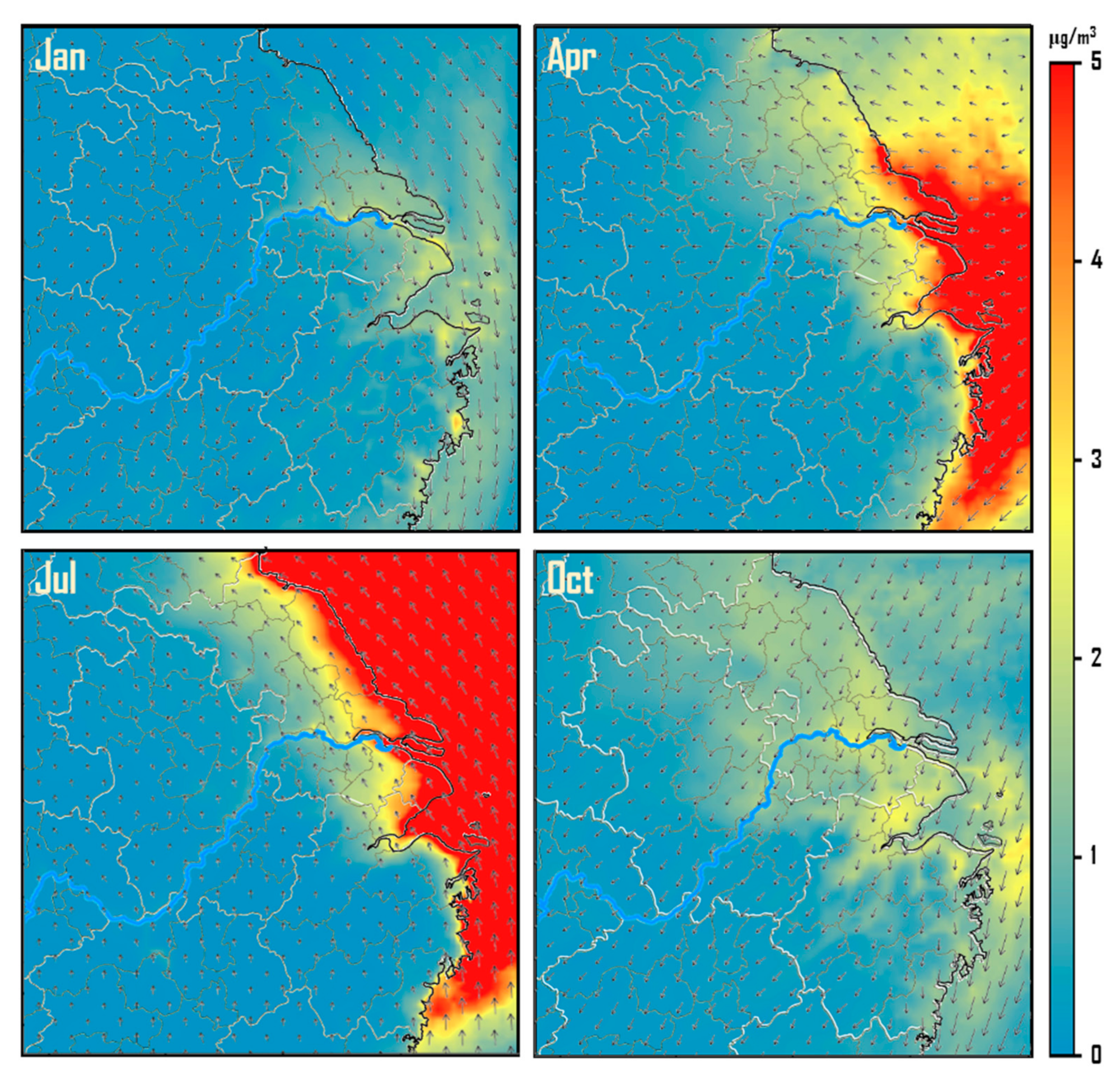
3.3. Changes in the Spatial Distribution

To identify the inter-annual changes in the spatial distribution of ship-contributed PM2.5 in YRD, the variation range where the contribution value exceeds a certain threshold will be investigated in this section. As shown in Figure 7, the spatial distribution of the 10-year average ship’s contribution is used as the base map, and the contour line where the concentration of ship-contributed PM2.5 equal to 1 μg/m3 was selected as the reference line for discussion, which is marked with a red bold line. The white shaded area overlapped on the base map indicates the inter-annual variation range of the 1 μg/m3 contour in the ten-year interval. For annual average on the left panel, it can be seen from the spatial range of the white shaded area that the area evidently affected by ships has very significant inter-annual changes (here, we specifically refer to the area where the contribution of PM2.5 exceeds 1 μg/m3), with the range of change in most areas ~80 km. However, the variation range of the seasonal average shown on the right panel was considerably higher than that of the annual average. For each season, the coverage of the white shaded area shows significant seasonal changes, not only the location of coverage but also the size of its own coverage. It was found that the coverage of the white shaded area located further inland region from coastline in spring and fall compared to winter and summer. This may be because the prevailing wind direction in spring and autumn was more perpendicular to the coastline than in winter and summer (as shown in Figure 5). It can also be seen from the figure that the fall was the season with the largest variation range among the four seasons. Furthermore, the variation range of the seasonal average in northern part of the YRD was considerably higher than that in the south. The topographic features in the study area provide clues to explain this spatial heterogeneity of the inter-annual variability. As showed in Figure 1, the southwest of YRD was dominated by hilly and mountainous areas with a high vegetation coverage, while most of the northern areas were mainly plains containing urban and farmland. Therefore, due to the obstacles of the hills and mountains in the southern YRD, ship emissions were more difficult to transport inland. On the contrary, because there was no blockage from high terrain in the northern YRD, ship emissions were more readily be transported inland, and may thus be more obviously affected by inter-annual changes in meteorological conditions.

4. Conclusions

In this study, the influence of inter-annual meteorological variation on the ship-contributed PM2.5 in YRD from 2010 to 2019. The emissions (emission inventory of 2014) and model configurations were kept the same over the study period, while the actual meteorological data for each year were used in the 10-year simulation to highlight the impact of inter-annual meteorological changes. The results indicate that ship emissions caused an evident increase in PM2.5, not only in port and coastal areas but also over wider inland regions. Generally, the simulated 10-year average ship contribution of PM2.5 to the whole land areas in YRD region was 1.41 μg/m3. It was up to 4.57 μg/m3 in coastal areas, and as the distance from the coastline increased, the contribution was reduced to less than 0.5 μg/m3 far inland. In coastal areas that were significantly affected by ship emissions, the influence along the northern coastline of YRD was much more evident than the southern coastline.
The ship-contributed PM2.5 in most coastal cities showed remarkable inter-annual fluctuation from 2010 to 2019 due to the inter-annual meteorological variation, especially in cities where the impact of ships emissions relatively more pronounced. It was also found that the inter-annual changes in ship’s contribution showed a trend of almost simultaneous increase and decrease for most cities, which indicates that the impact of inter-annual meteorological variation on the ship contribution was more regional than local.
The simulated 10-year average ship contribution in the four seasons showed that the ship’s impacts in spring and summer were more significant than that in fall and winter, and much sharper gradient of contributed PM2.5 was found near the coastline in spring and summer. The inter-annual changes of ship-contributed PM2.5 in different seasons were also significant, and exhibited dramatic seasonal difference. The most significant inter-annual change in the contribution of ships was found in summer, followed by spring, fall and winter. Similar to annual results, the inter-annual changes in the northern part of YRD in the four seasons were significantly higher than those in the south.
The inter-annual changes in the spatial distribution of ship-contributed PM2.5 in YRD were significant. The fall was the season with the largest variation range among the four seasons. In summer, the main changes mainly occurred in northern part of the YRD, and the changes in the southern area were relatively small.
These results indicate that: (1) compared with inland areas, coastal cities should pay more attention to the impact of ships, not only considering the average of their contributions, but also their inter-annual changes; (2) when assessing the ship’s impact, the uncertainty can be greatly reduced based on the multi-year average value than just based on a specific year; (3) when formulating ship control policies, cities in northern part of YRD should pay more attention to the impact of ships than the southern area; (4) among the four seasons, not only the absolute contribution value of ships in summer is the largest, but the inter-annual changes are also the most significant, which requires special attention; (5) compared with other coastal cities, cities with large ports should not only consider the absolute contribution of ships when formulating pollution control policies, but also pay attention to their inter-annual fluctuations. This is because under certain meteorological conditions in a certain year, the impact of ships may be significantly greater than the historical average. When formulating a control policy, it is necessary to consider the impact of uncertainty caused by this abnormal increase.
The research results of this article can provide meaningful references for those regions with similar climatic conditions, and within a certain confidence interval, analogies can be made based on the conclusions of this article. However, due to the strong nonlinearity and complexity of climate, these analogies will still bring certain uncertainty. For regions with very different climates, this uncertainty will be considerable. Therefore, for different regions, especially those regions with completely different climatic conditions from this study, it will be a better choice to use the method proposed in this article to carry out long-term local simulation analysis.

Author Contributions

Conceptualization, D.C.; Methodology, D.C.; Project administration, D.C. and L.L.; Validation, X.G., Y.Z. and J.L.; Formal Analysis, D.L.; Investigation, D.L.; Resources, L.L.; Data Curation, L.L.; Writing—Original Draft Preparation, D.L.; Writing—Review and Editing, D.C.; Visualization, D.L. All authors have read and agreed to the published version of the manuscript.

Funding

This research was funded by National Natural Science Foundation of China (No.51978011).

Institutional Review Board Statement

Not applicable.

Informed Consent Statement

Not applicable.

Data Availability Statement

The data presented in this study are openly available in references [43,46,47,68].

Acknowledgments

The authors are grateful to the anonymous reviewers for their insightful comments.

Conflicts of Interest

The authors declare no conflict of interest.

References

  1. Sorte, S.; Rodrigues, V.; Borrego, C.; Monteiro, A. Impact of harbour activities on local air quality: A review. Environ. Pollut. 2020, 257, 113542. [Google Scholar] [CrossRef] [PubMed]
  2. Ramacher, M.; Lin, T.; Moldanova, J.; Matthias, V.; Johansson, L. The impact of ship emissions on air quality and human health in the Gothenburg area -Part II: Scenarios for 2040. Atmos. Chem. Physics. 2020, 20, 10667–10686. [Google Scholar] [CrossRef]
  3. UNCTAD. Review of Maritime Transport 2019. Available online: https://unctad.org/system/files/official-document/rmt2019_en.pdf (accessed on 20 January 2020).
  4. Endresen, Y.; Srgrd, E.; Sundet, J.K.; Dalsren, S.B.; Isaksen, I.; Berglen, T.F.; Gravir, G. Emission from international sea transportation and environmental impact. J. Res. Atmos. 2003, 108, 4560. [Google Scholar] [CrossRef]
  5. Corbett, J.J.; Fischbeck, P. Emissions from ships. Science 1997, 278, 823–824. [Google Scholar] [CrossRef]
  6. Capaldo, K.; Corbett, J.J.; Kasibhatla, P.; Fischbeck, P.; Pandis, S.N. Effects of ship emissions on sulphur cycling and radiative climate forcing over the ocean. Nature 1999, 400, 743. [Google Scholar] [CrossRef]
  7. Sofiev, M.; Winebrake, J.J.; Johansson, L.; Carr, E.W.; Prank, M.; Soares, J.; Vira, J.; Kouznetsov, R.; Jalkanen, J.P.; Corbett, J.J. Cleaner fuels for ships provide public health benefits with climate tradeoffs. Nat. Commun. 2018, 9, 406. [Google Scholar] [CrossRef] [PubMed] [Green Version]
  8. Lv, Z.; Liu, H.; Ying, Q.; Fu, M.; Meng, Z.; Wang, Y.; Wei, W.; Gong, H.; He, K. Impacts of shipping emissions on PM2.5 pollution in China. Atmos. Chem. Phys. 2018, 18, 15811–15824. [Google Scholar] [CrossRef] [Green Version]
  9. Bie, S.; Yang, L.; Zhang, Y.; Huang, Q.; Li, J.; Zhao, T.; Zhang, X.; Wang, P.; Wang, W. Source appointment of PM2.5 in Qingdao Port, East of China. Sci. Total Environ. 2021, 755, 142456. [Google Scholar] [CrossRef]
  10. Lawrence, M.G.; Crutzen, P.J. Influence of NOx emissions from ships on tropospheric photochemistry and climate. Nature 1999, 402, 167–170. [Google Scholar] [CrossRef]
  11. Eyring, V.; Isaksen, I.S.; Berntsen, T.; Collins, W.J.; Corbett, J.J.; Endresen, O.; Grainger, R.G.; Moldanova, J.; Schlager, H.; Stevenson, D.S. Transport impacts on atmosphere and climate: Ship. Atmos. Environ. 2010, 44, 4735–4771. [Google Scholar] [CrossRef]
  12. Liu, H.; Fu, M.; Jin, X.; Shang, Y.; Shindell, D.; Faluvegi, G.; Shindell, C.; He, K. Health and climate impacts of oceangoing vessels in East Asia. Nat. Clim. Chang. 2016, 6, 1037–1041. [Google Scholar] [CrossRef]
  13. Thornton, J.A.; Virts, K.S.; Holzworth, R.H.; Mitchell, T.P. Lightning enhancement over major oceanic ship lanes. Geophys. Res. Lett. 2017, 44, 9102–9111. [Google Scholar] [CrossRef] [Green Version]
  14. Johansson, L.; Jalkanen, J.-P.; Kukkonen, J. Global assessment of ship emissions in 2015 on a high spatial and temporal resolution. Atmos. Environ. 2017, 167, 403–415. [Google Scholar] [CrossRef]
  15. Li, M.; Zhang, D.; Li, C.-T.; Mulvaney, K.M.; Selin, N.E.; Karplus, V.J. Air quality cobenefits of carbon pricing in China. Nat. Clim. Chang. 2018, 8, 398. [Google Scholar] [CrossRef]
  16. Wang, X.; Yi, W.; Lv, Z.; Deng, F.; Zheng, S.; Xu, H.; Zhao, J.; Liu, H.; He, K. Annual changes of ship emissions around China under gradually promoted control policies from 2016 to 2019. Atmos. Chem. Phys. Discuss. 2021. [preprint] in review. [Google Scholar] [CrossRef]
  17. Jonson, J.E.; Gauss, M.; Schulz, M.; Jalkanen, J.-P.; Fagerli, H. Effects of global ship emissions on European air pollution levels. Atmos. Chem. Phys. 2020, 20, 11399–11422. [Google Scholar] [CrossRef]
  18. Viana, M.; Hammingh, P.; Colette, A.; Querol, X.; Degraeuwe, B.; de Vlieger, I.; van Aardenne, J. Impact of maritime transport emissions on coastal air quality in Europe. Atmos. Environ. 2014, 90, 96–105. [Google Scholar] [CrossRef]
  19. Eyring, V.; Kohler, H.W.; Van Aardenne, J.; Lauer, A. Emissions from international shipping: 1. The last 50 years. J. Geophys. Res. Atmos. 2005, 110, 1984–2012. [Google Scholar] [CrossRef]
  20. Liu, H.; Meng, Z.H.; Shang, Y.; Lv, Z.F.; Jin, X.X. Shipping emission forecasts and cost-benefit analysis of China ports and key regions’ control. Environ. Pollut. 2018, 236, 49–59. [Google Scholar] [CrossRef]
  21. Liu, H.; Jin, X.; Wu, L.; Wang, X.; Fu, M.; Lv, Z.; Morawska, L.; Huang, F.; He, K. The impact of marine shipping and its DECA control on air quality in the Pearl River Delta, China. Sci. Total Environ. 2018, 625, 1476–1485. [Google Scholar] [CrossRef]
  22. UNCTAD. Review of Maritime Transport 2020. Available online: https://unctad.org/webflyer/review-maritime-transport-2020 (accessed on 10 March 2021).
  23. World Shipping Council. Available online: https://www.worldshipping.org/ (accessed on 10 March 2021).
  24. Liu, Z.; Lu, X.; Feng, J.; Fan, Q.; Zhang, Y.; Yang, X. Influence of Ship Emissions on Urban Air Quality: A Comprehensive Study Using Highly Time-Resolved Online Measurements and Numerical Simulation in Shanghai. Environ. Sci. Technol. 2017, 51, 202–211. [Google Scholar] [CrossRef]
  25. Zhao, J.; Zhang, Y.; Patton, A.; Ma, W.C.; Kan, H.D.; Wu, L.B.; Fung, F.; Wang, S.X.; Ding, D.; Walker, K. Projection of ship emissions and their impact on air quality in 2030 in Yangtze River delta, China. Environ. Pollut. 2020, 263, 114643. [Google Scholar] [CrossRef] [PubMed]
  26. Zhang, Y.; Yang, X.; Brown, R.; Yang, L.; Morawska, L.; Ristovski, Z.; Fu, Q.; Huang, C. Shipping emissions and their impacts on air quality in China. Total Environ. 2017, 581, 186–198. [Google Scholar] [CrossRef] [PubMed]
  27. Fu, M.; Liu, H.; Jin, X.; He, K. National- to port-level inventories of shipping emissions in China. Environ. Res. Lett. 2017, 12, 114024. [Google Scholar] [CrossRef]
  28. Wang, X.; Shen, Y.; Lin, Y.; Pan, J.; Zhang, Y.; Louie, P.K.; Li, M.; Fu, Q. Atmospheric pollution from ships and its impact on local air quality at a port site in Shanghai. Atmos. Chem. Phys. 2019, 19, 6315–6330. [Google Scholar] [CrossRef] [Green Version]
  29. Mamoudou, I.; Zhang, F.; Chen, Q.; Wang, P.; Chen, Y. Characteristics of PM2.5 from ship emissions and their impacts on the ambient air: A case study in Yangshan Harbor, Shanghai. Total Environ. 2018, 640–641, 207–216. [Google Scholar] [CrossRef]
  30. Zhao, M.; Zhang, Y.; Ma, W.; Fu, Q.; Xin, Y.; Li, C.; Zhou, B.; Qi, Y.; Chen, L. Characteristics and ship traffic source identification of air pollutants in China’s largest port. Atmos. Environ. 2013, 64, 277–286. [Google Scholar] [CrossRef]
  31. Fu, M.L.; Ding, Y.; Ge, Y.S.; Yu, L.X.; Yin, H.; Ye, W.T.; Liang, B. Real-world emissions of inland ships on the Grand Canal, China. Atmos. Environ. 2013, 81, 222–229. [Google Scholar] [CrossRef]
  32. Fan, Q.; Zhang, Y.; Ma, W.; Ma, H.; Feng, J.; Yu, Q.; Yang, X.; Ng, S.K.; Fu, Q.; Chen, L. Spatial and seasonal dynamics of ship emissions over the Yangtze river delta and east China sea and their potential environmental influence. Environ. Sci. Technol. 2016, 50, 1322–1329. [Google Scholar] [CrossRef]
  33. Chen, D.S.; Tian, X.X.; Lang, J.L.; Zhou, Y.; Li, Y.; Guo, X.R.; Wang, W.L.; Liu, B. The impact of ship emissions on PM2.5 and the deposition of nitrogen and sulfur in Yangtze River Delta, China. Sci. Total Environ. 2019, 649, 1609–1619. [Google Scholar] [CrossRef]
  34. Feng, J.; Zhang, Y.; Shanshan, L.; Mao, J.; Patton, A.; Zhou, Y.; Ma, W.; Liu, C.; Shen, Y.; Fu, Q.; et al. The influence of spatiality on shipping emissions, air quality and potential human exposure in the Yangtze River Delta/Shanghai, China. Atmos. Chem. Phys. 2019, 19, 6167–6183. [Google Scholar] [CrossRef] [Green Version]
  35. Zhai, S.; Daniel, J.J.; Wang, X.; Shen, L.; Zhang, Y.; Gui, K.; Zhao, T.; Liao, L.; Zhai, S. Fine particulate matter (PM2.5) trends in China, 2013–2018: Separating contributions from anthropogenic emissions and meteorology. Atmos. Chem. Phys. 2019, 19, 11031–11041. [Google Scholar] [CrossRef] [Green Version]
  36. Xu, Y.; Xue, W.; Lei, Y.; Huang, Q.; Zhao, Y.; Zhao, Y.; Cheng, S.; Ren, Z.; Wang, J. Spatiotemporal variation in the impact of meteorological conditions on PM2.5 pollution in China from 2000 to 2017. Atmos. Environ. 2020, 223, 117215. [Google Scholar] [CrossRef]
  37. Ghude, S.; Chate, D.; Jena, C.; Beig, G.; Kumar, R.; Barth, M.; Pfister, G.; Fadnavis, S.; Pithani, P. Premature mortality in India due to PM2.5 and ozone exposure. Geophys. Res. Lett. 2016, 43, 4650–4658. [Google Scholar] [CrossRef] [Green Version]
  38. Mahmud, A.; Hixson, M.; Kleeman, M.J. Quantifying population exposure to airborne particulate matter during extreme events in California due to climate change. Atmos. Chem. Phys. 2012, 12, 7453–7463. [Google Scholar] [CrossRef] [Green Version]
  39. USEPA. Air Quality Criteria for Ozone and Related Photochemical Oxidants; US Environmental Protection Agency: Washington, DC, USA, 2006. [Google Scholar]
  40. Zhang, H.; Wang, Y.; Hu, J.; Qi, Y.; Hu, X.M. Relationships between meteorological parameters and criteria air pollutants in three megacities in China. Environ. Res. 2015, 140, 242–254. [Google Scholar] [CrossRef]
  41. Zhang, Q.; Ma, Q.; Zhao, B.; Liu, X.; Wang, Y. Winter haze over North China Plain from 2009 to 2016: Influence of emission and meteorology. Environ. Pollut. 2018, 242, 1308–1318. [Google Scholar] [CrossRef]
  42. Shang, F.; Chen, D.C.; Guo, X.R.; Lang, J.L.; Zhou, Y.; Li, Y.; Fu, X.Y. Impact of Sea Breeze Circulation on the Transport of Ship Emissions in Tangshan Port, China. Atmosphere 2019, 10, 723. [Google Scholar] [CrossRef] [Green Version]
  43. China Meteorological Administration. Available online: http://data.cma.cn/ (accessed on 10 May 2021).
  44. Liao, Z.; Gao, M.; Sun, J.; Fan, S. The impact of synoptic circulation on air quality and pollution-related human health in the Yangtze River Delta region. Sci. Total Environ. 2017, 607, 838–846. [Google Scholar] [CrossRef]
  45. Daoyi, G.; Jinhong, Z.; Shaowu, W. The Influence of Siberian High on Large-Scale Climate over Continental Asia. Plateau Meteorol. 2002, 21, 9–13. [Google Scholar]
  46. Shanghai Environmental Protection Bureau. Available online: https://sthj.sh.gov.cn/hbzhywpt1143/hbzhywpt1144/index.html (accessed on 10 May 2021).
  47. Ministry of Ecology and Environmental of the People’s Republic. Ecological and Environmental Bulletin. Available online: http://www.mee.gov.cn/hjzl/ (accessed on 10 May 2021).
  48. Kang, H.; Zhu, B.; Gao, J.; He, Y.; Wang, H.; Su, J.; Pan, C.; Zhu, T.; Yu, B. Potential impacts of cold frontal passage on air quality over the Yangtze River Delta, China. Atmos. Chem. Phys. 2019, 19, 3673–3685. [Google Scholar] [CrossRef] [Green Version]
  49. Wong, H.L.A.; Wang, T.; Ding, A.; Blake, D.R.; Nam, J.C. Impact of Asian continental outflow on the concentrations of O3, CO, NMHCs and halocarbons on Jeju Island, South Korea during March 2005. Atmos. Environ. 2007, 41, 2933–2944. [Google Scholar] [CrossRef] [Green Version]
  50. Wang, T.; Ding, A.; Blake, D.R.; Zahorowski, W.; Poon, C.N.; Li, Y.S. Chemical characterization of the boundary layer outflow of air pollution to Hong Kong during February-April 2001. Geophys. Res. 2003, 108, 8787. [Google Scholar] [CrossRef] [Green Version]
  51. Qu, Y.; Ma, J.; Xu, J.; Zhong, Q.; Mao, Z.; Zhou, W. Application of meteorological air pollution index in Shanghai. Meteorol. Mon. 2018, 44, 704–712. (In Chinese) [Google Scholar]
  52. Caiyanlin, Z.Z.F. Numerical Simulations of an Advection Fog Event over Shanghai Pudong International Air-port with the WRF Model. J. Meteorol. Res. 2017, 31, 874–889. [Google Scholar]
  53. Xue, W.; Shi, X.; Yan, G.; Wang, J.; Xu, Y.; Tang, Q.; Wang, Y.; Zheng, Y.; Lei, Y. Impacts of meteorology and emission variations on the heavy air pollution episode in North China around the 2020 Spring Festival. China Earth Sci. 2021, 64, 329–339. [Google Scholar] [CrossRef]
  54. Samaali, M.; Moranl, D.M.; Bouchet, V.S.; Pavlovic, R.; Cousineau, S.; Sassi, M. On the influence of chemical initial and boundary conditions on annual regional air quality model simulations for North America. Atmos. Environ. 2009, 43, 4873–4885. [Google Scholar] [CrossRef]
  55. Wang, X.; Zhang, R. Effects of atmospheric circulations on the interannual variation in PM2.5 concentrations over the Beijing–Tianjin–Hebei region in 2013–2018. Atmos. Chem. Phys. 2020, 20, 7667–7682. [Google Scholar] [CrossRef]
  56. Mao, J.; Zhang, Y.; Yu, F.; Chen, J.; Sun, J.; Wang, S.; Zou, Z.; Zhou, J.; Yu, Q.; Ma, W.; et al. Simulating the impacts of ship emissions on coastal air quality: Importance of a high-resolution emission inventory relative to cruise- and land-based observations. Sci. Total Environ. 2020, 728, 138454. [Google Scholar] [CrossRef] [PubMed]
  57. Zheng, H.; Cai, S.; Wang, S.; Zhao, B.; Chang, X.; Hao, J. Development of a unit-based industrial emission inventory in the Beijing–Tianjin–Hebei region and resulting improvement in air quality modelling. Atmos. Chem. Phys. 2019, 19, 3447–3462. [Google Scholar] [CrossRef] [Green Version]
  58. Zhang, H.; Cheng, S.; Yao, S.; Wang, X.; Zhang, J. Multiple perspectives for modelling regional PM2.5 transport across cities in the Beijing–Tianjin–Hebei region during haze episodes. Atmos. Environ. 2019, 212, 22–35. [Google Scholar] [CrossRef]
  59. Yang, X.; Wu, Q.; Zhao, R.; Cheng, H.; He, H.; Ma, Q.; Wang, L.; Luo, H. New method for evaluating winter air quality: PM2.5 assessment using Community Multi-Scale Air Quality Modelling (CMAQ) in Xi’an. Atmos. Environ. 2019, 211, 18–28. [Google Scholar] [CrossRef]
  60. Lin, Y.; Farley, R.; Orville, H. Bulk Parameterization of the snow field in a cloud model. Clim. Appl. Meteorol. 1983, 22, 1065–1092. [Google Scholar] [CrossRef] [Green Version]
  61. Tewari, M.; Chen, F.; Wang, W.; Dudhia, J.; LeMone, M.A.; Mitchell, K.; Ek, M.; Gayno, G.; Wegiel, J.; Cuenca, R.H. Implementation and Verification of the Unified NOAH Land Surface Model in the WRF Model. In Proceedings of the 20th Conference on Weather Analysis and Forecasting/16th Conference on Numerical Weather Prediction, Seattle, WA, USA, 10 January 2004; pp. 11–15. [Google Scholar]
  62. Hong, S.-Y.; Yign, N.; Jimy, D. A new vertical diffusion package with an explicit treatment of entrainment processes. Mon. Wea. Rev. 2006, 134, 2318–2341. [Google Scholar] [CrossRef] [Green Version]
  63. Chou, M.D.; Suarez, M.J.; Liang, X.Z.; Yan, M.M.H. A thermal infrared radiation parameterization for atmospheric studies. NASA Tech. Memo. 2001, 19, 1–68. [Google Scholar]
  64. Stephen., F.B.; Schwarzkopf, M.D. An efficient, accurate algorithm for calculating CO2 15 µm band cooling rates. Geophys. Res. 1981, 86, 1205–1232. [Google Scholar]
  65. Sarwar, G.; Luecken, D.; Yarwood, G.; Whitten, G.Z.; Carter, W.P.L. Impact of an updated carbon bond mechanism on predictions from the CMAQ modeling system: Preliminary assessment. J. Appl. Meteorol. Clim. 2008, 47, 3–14. [Google Scholar] [CrossRef]
  66. Whitten, G.Z.; Heo, G.; Kimura, Y.; McDonald-Buller, E.; Allen, D.T.; Carter, W.P.L.; Yarwood, G. A new condensed toluene mechanism for Carbon Bond: CB05-TU. Atmos. Environ. 2010, 44, 5346–5355. [Google Scholar] [CrossRef]
  67. Yarwood, G.; Jung, J.; Heo, G.; Whitten, G.Z.; Mellberg, J.; Estes, M. CB06-version 6 of the carbon bond mechanism. In Proceedings of the 2010 CMAS Conference, Chapel Hill, NC, USA, 11 October 2010. [Google Scholar]
  68. NCEP. Available online: https://rda.ucar.edu/datasets/ds083.2/ (accessed on 12 February 2020).
  69. Chen, D.; Wang, X.; Li, Y.; Lang, J.; Zhou, Y.; Guo, X.; Zhao, Y. High-spatiotemporal-resolution ship emission inventory of China based on AIS data in 2014. Sci. Total Environ. 2017, 609, 776–787. [Google Scholar] [CrossRef] [PubMed]
  70. Zhang, Q.; Streets, D.G.; Carmichael, G.R.; He, K.B.; Huo, H.; Kannari, A.; Klimont, Z.; Park, I.S.; Reddy, S.; Fu, J.S.; et al. Asian emissions in 2006 for the NASA INTEX-B mission. Atmos. Chem. Phys. 2009, 9, 5131–5153. [Google Scholar] [CrossRef] [Green Version]
  71. Li, M.; Zhang, Q.; Streets, D.G.; He, K.B.; Cheng, Y.F.; Emmons, L.K.; Huo, H.; Kang, S.C.; Lu, Z.; Shao, M. Mapping Asian anthropogenic emissions of non-methane volatile organic compounds to multiple chemical mechanisms. Atmos. Chem. Phys. 2014, 14, 5617–5638. [Google Scholar] [CrossRef] [Green Version]
  72. Zheng, B.; Huo, H.; Zhang, Q.; Yao, Z.L.; Wang, X.T.; Yang, X.F.; Liu, H.; He, K.B. High–resolution mapping of vehicle emissions in China in 2008. Atmos. Chem. Phys. 2014, 14, 9787–9805. [Google Scholar] [CrossRef] [Green Version]
  73. Liu, F.; Zhang, Q.; Tong, D.; Zheng, B.; Li, M.; Huo, H.; He, K.B. High-resolution inventory of technologies, activities, and emissions of coal-fired power plants in China from 1990 to 2010. Atmos. Chem. Phys. 2015, 15, 13299–13317. [Google Scholar] [CrossRef] [Green Version]
  74. Zhou, Y.; Xing, X.; Lang, J.; Chen, D.; Cheng, S.; Wei, L.; Wei, X.; Liu, C. A comprehensive biomass burning emission inventory with high spatial and temporal resolution in China. Atmos. Chem. Phys. 2017, 17, 2839–2864. [Google Scholar] [CrossRef] [Green Version]
  75. Chen, D.S.; Cheng, S.Y.; Li, J.B.; Chen, T.; Zhao, X.Y.; Guo, X.R.; Hu, H.L.; Yu, T. Application of LIDAR Technique and MM5-CMAQ Modeling Approach for the Assessment of Winter PM10 Air Pollution: A Case Study in Beijing, China. Water Air Soil Pollut. 2007, 181, 409–427. [Google Scholar] [CrossRef]
  76. Chen, D.S.; Cheng, S.Y.; Liu, L.; Chen, T.; Guo, X.R. An integrated MM5–CMAQ modeling approach for assessing trans-boundary PM10 contribution to the host city of 2008 Olympic summer games-Beijing, China. Atmos. Environ. 2007, 41, 1237–1250. [Google Scholar] [CrossRef]
  77. Chen, D.S.; Cheng, S.Y.; Liu, L.; Lei, T.; Guo, X.R.; Zhao, X.Y. Assessment of the Integrated ARPS-CMAQ Modeling System through Simulating PM10 Concentration in Beijing. China. Environ. Eng. Sci. 2008, 25, 191–206. [Google Scholar] [CrossRef]
  78. Chen, D.; Cheng, S.; Zhou, Y.; Guo, X.; Fan, S.; Wang, H. Impact of Road Fugitive Dust on Air Quality in Beijing. China. Environ. Eng. Sci. 2010, 27, 825–834. [Google Scholar] [CrossRef]
  79. Chen, D.S.; Wang, X.T.; Nelson, P.; Li, Y.; Zhao, N.; Zhao, Y.H.; Lang, J.L.; Zhou, Y.; Guo, X.R. Ship emission inventory and its impact on the PM2.5 air pollution in Qingdao Port, North China. Atmos. Environ. 2017, 166, 351–361. [Google Scholar] [CrossRef]
  80. Chen, D.S.; Liu, X.X.; Lang, J.L.; Zhou, Y.; Wei, L.; Wang, X.T.; Guo, X.R. Estimating the contribution of regional transport to PM2.5 air pollution in a rural area on the North China Plain. Sci. Total Environ. 2017, 583, 280–291. [Google Scholar] [CrossRef] [PubMed]
  81. Chen, D.S.; Zhao, N.; Lang, J.L.; Zhou, Y.; Wang, X.T.; Li, Y.; Zhao, Y.H.; Guo, X.R. Contribution of ship emissions to the concentration of PM2.5: A comprehensive study using AIS data and WRF/Chem model in Bohai Rim Region, China. Sci. Total Environ. 2018, 610, 1476–1486. [Google Scholar] [CrossRef] [PubMed]
  82. Chen, D.; Fu, X.; Guo, X.; Lang, J.; Zhou, Y.; Li, Y.; Liu, B.; Wang, W. The impact of ship emissions on nitrogen and sulfur deposition in China. Sci. Total Environ. 2020, 708, 124636. [Google Scholar] [CrossRef]
  83. Chen, D.; Zhang, Y.; Lang, J.; Ying, Z.; Li, Y.; Guo, X.; Wang, W.; Liu, B. Evaluation of different control measures in 2014 to mitigate the impact of ship emissions on air quality in the Pearl River Delta, China. Atmos. Environ. 2019, 216, 116911. [Google Scholar] [CrossRef]
  84. Han, X.; Zhang, M.; Skorokhod, A.; Kou, X. Modeling dry deposition of reactive nitrogen in China with RAMS-CMAQ. Atmos. Environ. 2017, 166, 47–61. [Google Scholar] [CrossRef]
  85. Li, R.; Zhang, M.; Chen, L.; Kou, X.; Skorokhod, A. CMAQ simulation of atmospheric CO2 concentration in East Asia: Comparison with GOSAT observations and ground measurements. Atmos. Environ. 2017, 160, 176–185. [Google Scholar] [CrossRef]
  86. Wang, L.; Wei, Z.; Wei, W.; Fu, J.S.; Meng, C.; Ma, S. Source apportionment of PM2.5 in top polluted cities in Hebei, China using the CMAQ model. Atmos. Environ. 2015, 122, 723–736. [Google Scholar] [CrossRef]
  87. Constantinidou, K.; Hadjinicolaou, P.; Zittis, G.; Lelieveld, J. Performance of Land Surface Schemes in the WRF Model for Climate Simulations over the MENA-CORDEX Domain. Earth Syst. Environ. 2020, 4, 1–19. [Google Scholar] [CrossRef]
  88. NCEI. Available online: https://gis.ncdc.noaa.gov/maps/ncei/cdo/hourly/ (accessed on 20 July 2020).
  89. Boylan, J.W.; Russell, A.G. PM and light extinction model performance metrics, goals, and criteria for three-dimensional air quality models. Atmos. Environ. 2006, 40, 4946–4959. [Google Scholar] [CrossRef]
  90. Liu, X.; Zhu, B.; Kang, H.; Hou, X.; Gao, J.; Kuang, X.; Yan, S.; Shi, S.; Fang, C.; Pan, C.; et al. Stable and transport indices applied to winter air pollution over the Yangtze River Delta, China. Environ. Pollut. 2021, 272, 115954. [Google Scholar] [CrossRef] [PubMed]
  91. Webster, P.J.; Magana, V.O.; Palmer, T.N.; Shukla, J.; Tomas, R.A.; Yanai, M.; Yasunari, T. Monsoons: Processes, predictability, and the prospects for prediction. J. Geophys. Res. 1998, 103, 14451–14510. [Google Scholar] [CrossRef]
  92. Li, J.; Zeng, Q.A. Unified monsoon index. Geophys. Res. Lett. 2020, 29, 1274. [Google Scholar] [CrossRef]
  93. Li, J.; Zeng, Q.A. A new monsoon index and the geographical distribution of the global monsoons. Adv. Atmos. Sci. 2003, 20, 299–302. [Google Scholar]
  94. Li, J.; Zeng, Q.A. A new monsoon index, its interannual variability and relation with monsoon precipitation. Clim. Environ. Res. 2005, 10, 351–365. [Google Scholar]
  95. Chen, G.; Du, Y.; Wen, Z. Seasonal, Interannual, and Interdecadal Variations of the East Asian Summer Monsoon: A Diurnal-Cycle Perspective. J. Clim. 2021, 34, 4403–4421. [Google Scholar] [CrossRef]
  96. Huang, R.H.; Chen, J.L.; Wang, L.; Lin, Z.D. Characteristics, processes, and causes of the spatio-temporal variabilities of the East Asian monsoon system. Adv. Atmos. Sci. 2012, 29, 910–942. [Google Scholar] [CrossRef]
  97. Huang, R.H.; Gu, L.; Xu, Y.H.; Zhang, Q.L.; Wu, S.S.; Cao, J. Characteristics of the interannual variations of onset and advance of the East Asian summer monsoon and their associations with thermal states of the tropical western Pacific. Chin. Atmos. Sci. 2005, 29, 20–36. (In Chinese) [Google Scholar]
  98. Zhang, L.; Liao, H.; Li, J. Impacts of Asian summer monsoon on seasonal and interannual variations of aerosols over eastern China. Geophys. Res. 2010, 115, D00K05. [Google Scholar] [CrossRef] [Green Version]
  99. Cheng, X.; Zhao, T.; Gong, S.; Xu, X.; Han, Y.; Yin, Y.; Tang, L.; He, H.; He, J. Implications of East Asian summer and winter monsoons for interannual aerosol variations over central-eastern China. Atmos. Environ. 2016, 129, 218–228. [Google Scholar] [CrossRef]
Figure 1. Sketch map of the study area and two nested domains established for modeling.
Atmosphere 12 00722 g001
Figure 2. Spatial distribution of annual ship emissions for different pollutions (kg/km2/yr) in 2014 over the YRD region.
Atmosphere 12 00722 g002
Figure 3. The 10-year average contribution of ship emissions to PM2.5 overlapped by wind vectors in µg/m3 (a) and in % (b) over YRD region, and the inter-annual variation of the contribution in 14 coastal cities from 2010 to 2019 (c).
Atmosphere 12 00722 g003
Figure 4. Anomalies of ship-contributed PM2.5 (μg/m3) and all PM2.5 pollution (ships + other sources) based on the annual average of each year, and the 10-year average of ship-contributed PM2.5 (μg/m3) in 14 coastal cities of YRD.
Atmosphere 12 00722 g004
Figure 5. The 10-year average contribution of ship emissions (μg/m3) to PM2.5 overlapped by wind vectors in YRD region in January, April, July and October, which represent the four seasons of winter, summer, fall and spring, respectively.
Atmosphere 12 00722 g005
Figure 6. Anomalies of ship-contributed PM2.5 (μg/m3) based on the seasonal average of each year and the 10-year average in coastal cities of YRD in January, April, July and October, which represent the four seasons of winter, summer, fall and spring, respectively.
Atmosphere 12 00722 g006
Figure 7. The inter-annual variation ranges of distribution of annual and seasonal ship-contributed PM2.5 in YRD.
Atmosphere 12 00722 g007
Table 1. Performance statistics for temperature at 2 m (T2), relative humidity at 2 m (RH2), wind speed at 10 m (WS10) at 150 sites within the study area.
SpeciesMonthAVG-obs 1AVG-sim 2MAE 3R 4
T2January6.225.611.280.84
April15.4213.861.990.81
July27.2326.491.460.78
October19.7918.891.380.87
RH2January70.3171.118.270.75
%April76.2880.628.360.83
July82.9489.957.570.72
October72.2277.608.200.73
WS10January2.783.120.860.72
m/sApril3.233.432.460.75
July2.853.320.950.74
October3.083.310.890.78
1 AVG-obs indicates the Average in Observations. 2 AVG-sim indicates the Average in Simulations. 3 MAE indicates the Mean Absolute Error. 4 R indicates the correlative coefficient.
Table 2. Performance statistics for PM2.5, PM10, SO2, NO2, O3 concentrations at 171 sites within the study area.
SpeciesMonthMAENMB 5 (%)NME 6 (%)MFB 7 (%)MFE 8 (%)R
PM2.5January21.19−9.3325.29−5.8917.270.84
µg/m3April12.81−4.3717.49−3.1512.140.81
July13.22−10.2332.03−10.8026.510.75
October14.15−27.7029.29−21.9623.320.78
PM10January22.09−8.6318.87−5.9215.220.83
µg/m3April15.38−3.2118.66−2.2013.680.73
July16.93−4.6524.85−6.0620.400.76
October16.25−5.6019.27−6.0015.840.82
SO2January9.773.0031.671.6023.470.76
µg/m3April5.671.6228.151.8419.690.77
July3.74−2.5826.49−4.3520.640.72
October6.06−4.3029.21−6.7323.470.77
NO2January10.131.8319.942.5214.510.78
µg/m3April8.90−6.5420.01−6.4516.340.76
July8.49−17.6527.09−17.3824.280.77
October10.56−6.3824.88−7.2221.750.76
O3January9.04−4.4215.30−4.0011.390.76
µg/m3April11.64−4.7711.35−4.408.770.74
July22.04−11.0518.20−6.7313.710.82
October19.63−8.0815.97−6.8212.580.74
5 NMB indicates the Normalized Mean Bias. 6 NME indicates the Normalized Mean Error. 7 MFB: indicates the Mean Fractional Bias. 8 MFE: indicates the Mean Fractional Error.
Publisher’s Note: MDPI stays neutral with regard to jurisdictional claims in published maps and institutional affiliations.

