1. Introduction
Since limited-area mesoscale numerical weather prediction (NWP) modeling now has sufficient computational power at its disposal to achieve kilometer-scale grid spacing nesting, interest has grown rapidly in both the research and operational modeling communities to resolve flow features which have historically been only partially resolvable (or completely sub-grid scale) in traditional mesoscale NWP. Many of these phenomena are of interest to both civilian and military interests (wind and solar energy, air quality, fire weather, aviation and small unmanned aerial systems, urban activities, electromagnetic and acoustic propagation, transportation, and agriculture). For example, features such as mountain-valley wind systems [
1,
2], nocturnal interactions between katabatic, gap and valley flows [
3], slope flow separation important to orographic convection [
4], shallow boundary layer cumulus [
5], orographic lee waves [
6], radiation fog and cold pooling [
7], sea, lake and playa breezes [
8,
9], terrain and cloud shadowing [
10,
11], as well as organization of horizontal/longitudinal roll and cellular structures in the convective boundary layer [
12,
13,
14,
15,
16,
17,
18,
19]. These features are all best resolved at near-kilometer or sub-kilometer grid spacing, since additional resolution in terrain, land surface, and soil properties are necessary to capture the important details in the lower boundary forcing responsible for driving the local and regional heterogeneous variations of thermodynamic and flow properties responsible for their existence.
Other than within the extent of specialized field study campaigns, until fairly recently, routine measurements of these types of mesoscale structures were hampered due to limitations of spatial and temporal resolution in the routine observation network. This has led to challenges in evaluating the quality and value of models running at such scales [
20,
21]. Certain mesoscale structures such as horizontal convective rolls (HCR) have been studied more frequently in campaigns over generally flat or gently sloping terrain environments versus in complex terrain regions with steep slope features [
16,
22], although a variable range of terrain complexity can be expected to strongly modify behaviors of convection versus the flat terrain counterpart [
19]. The advent of Doppler radar and Doppler Light Detection and Ranging (LiDAR) (both ground-based and airborne) has been able to make measurements at such scales finally more achievable, including over extended collection periods. For example, recent studies exist in leveraging both Doppler weather radar and airborne Doppler LiDAR technology for studying both the climatology and physical characterization of the boundary layer (BL) HCR (also referred to as organized large eddy) structures [
16,
23].
A challenge for mesoscale NWP models nesting to around a kilometer (and especially sub-kilometer) grid spacing is that these resolutions fall into a well-known “terra incognita” gray area for traditional BL turbulence parameterization. The general range of grid spacing between about 100 m to 1 km cannot be completely addressed by either traditional mesoscale BL turbulence parameterization or large eddy simulation [
24]. Within this range, assumptions that are used to justify mesoscale BL parameterizations are not so easily defensible, since only a few large turbulent plumes (at best) might be contained within a single grid box. As the grid spacing gets down to a few hundred meters, this problem becomes even worse. These parameterizations were developed based on the assumption of there being many subgrid plumes within a grid box, and on the statistics of these plumes. At coarser grid spacing such as used by a global model, this assumption is quite valid. However, at kilometer and below grid spacing, individual very large plumes might become partially resolvable. On the other hand, a grid spacing larger than about 50 m becomes less suitable for use in a large eddy simulation, where the largest energy-containing turbulence is assumed resolved and only the Kolmogorov-scale smallest turbulence is parameterized.
Additional complications in the NWP turbulence gray area can exist due to improper choices of appropriate vertical resolution and shallow cumulus treatment, implicit diffusion of advection schemes, explicit numerical filtering choices, and terrain averaging methods [
25,
26]. Diffusion, filtering, and terrain averaging effects in a mesoscale NWP model can make the effective resolution more on the order of approximately seven times the grid spacing [
27]. When running mesoscale models at sub-kilometer grid spacing using a BL turbulence parameterization, modeled convectively-induced secondary circulations (such as rolls and cells) tend to become grid size-dependent [
28,
29]. Whether scale-aware turbulence parameterization approaches can address this issue effectively is still an area of active research [
28,
29,
30,
31,
32,
33,
34,
35]. The scale-aware approaches for the BL turbulence gray area attempt to adjust contributions between resolved and parameterized based on grid spacing, similar to how deep cumulus parameterization schemes have adopted scale-aware approaches for the cumulus parameterization gray area from 1 km to 10 km [
36].
Linearly elongated bands of enhanced upward vertical motion within the BL, which will be referred to hereafter as Longitudinal Roll Structures (LRS), were initially observed in runs of the National Center for Atmospheric Research’s (NCAR) Advanced Research version of the Weather Research and Forecast model (WRF-ARW; from here out referred to as just WRF). The LRS were noted when model nest resolutions approached about 1 km grid spacing and appeared to be afternoon features on spring days when there was strong southwesterly flow aloft and neutral-to-weakly unstable BL conditions (usually due to an approaching mid-tropospheric shortwave from the west). These model runs were centered over the Jornada Experimental Range (JER), New Mexico (NM) and initially served to investigate local mesoscale flow phenomena that might steer or impact future nowcasting or JER research efforts [
37]. Since the LRS appeared at 1 km grid spacing in WRF, which is at the very edge of the BL turbulence gray area, special care does need to be taken in interpreting these features based on the previous discussion regarding BL turbulence parameterization.
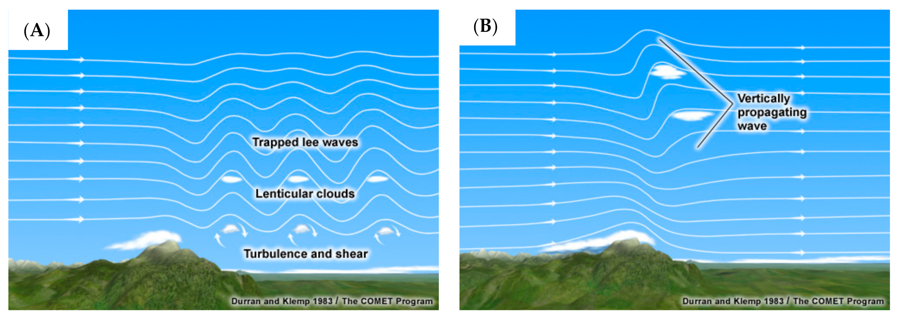
The spring case days where LRS were noted in this study also appeared to coincide with conditions favorable for lee wave formation across both the JER and the Tularosa Basin (TUL). The TUL spans between the San Andres Mountains (and Organ Mountains) and the Sacramento Mountains, from west-to-east respectively. When the atmosphere is stably stratified in the presence of synoptic forcing (such as a deepening mid-tropospheric shortwave approaching from the west in NM), a parcel of air encountering a topographical barrier can induce a buoyancy perturbation. This perturbation initiates an oscillatory behavior of that air parcel with wavelengths from 5 to 35 km, forming orographic lee waves. If sufficient moisture is present as the lee waves propagate downstream, lenticular cloud formation can occur as shown in
Figure 1A [
38]. Lee waves can propagate either horizontally, downwind, or vertically if the energy is trapped, and examples of both can be seen in
Figure 1. The presence of both lee waves and the LRS add complexity not always found in earlier studies of HCRs.
The LRS patterns piqued added interest due to their correlation with similarly elongated linear streaks previously observed in the topsoil layer in the JER northeast of the Doña Ana Mountains.
Figure 2A shows the LRS, which appear similar to HCR [
39] and the corresponding longitudinal soil bands observed in a Google Earth image in
Figure 2B. The similarity in location of these linear atmospheric and surface soil/vegetation patterns encouraged our further investigation.
Early in analysis the LRS presented as horizontal bands of decreased surface horizontal wind velocity (
) with enhanced upward vertical motion (
) throughout the BL. The enhanced upward plumes along the modeled LRS appeared to span the depth of the BL. After discovering the LRS in the preliminary model simulations [
37], synoptically similar days were chosen (12/04, 17/04, 20/04) in the spring of 2018 (which also overlapped a special field campaign ongoing over the JER). Upon preliminary inspection, LRS were observed on all three case study days within the WRF model simulations. This warranted us to apply more focus upon the modeled LRS, which is the primary focus of this paper. If such LRS do commonly exist seasonally over JER and TUL in a climatological sense, they could provide a potential mechanism for creating the soil patterns noted in
Figure 2B. That is, increased soil transport may occur in bands aligned with the dominant wind direction during synoptically forced periods.
2. Methods
The study domain was centered northeast of Las Cruces, NM, to include the southern half of NM due to the unique topography of the region as seen in
Figure 3A where towering mountains reach up to 2.4 km above the valley basins. Of particular interest is the San Andres Mountain range which extends approximately 120 km in the NW-SE direction and 20 km in the SW-NE direction. To the west of the San Andres lies the United States Department of Agriculture (USDA) Agricultural Research Service JER, a valley approximately 780 km
2 in size at an elevation of 1320 m, and to the east lies the TUL, approximately 16,800 km
2 at an elevation of 1200 m, bounded on either side by substantial mountain ranges. The TUL is bound to the east by the Sierra Blanca Peak (3650 m) and the Sacramento Mountains (2960 m) and to the west by the San Andres (2520 m) and Organ Mountains (2740 m). The JER and TUL basins are mostly flat and primarily desert shrub and grasslands, with the exception of the TUL that has a 65 km lava ribbon that runs through it and the white gypsum sands of the White Sands National Park (WSNP).
The United States Army Research Laboratory’s (ARL) Meteorological Sensor Array (MSA) consists of 62 meteorological towers that are distributed across the complex terrain of the JER as shown in
Figure 3A, which shows the locations of the MSA towers. The 10 m towers (green markers, shown in
Figure 3B) have instrumentation levels at 2 and 10 m, and the 30 m towers (blue markers) have instrumentation levels at 2, 4, 8, 16, 20, and 28 m. A typical MSA instrumentation level consists of a Gill Instruments Windmaster 3D sonic anemometer that measures the
,
,
components of velocity and sonic temperature at 20 Hz, and a Campbell Scientific 107 temperature probe or a Rotronics Hydroclip HC2S3-L temperature and relative humidity probe sampling at 1 Hz. The Data acquisition systems consist of a Campbell Scientific CR6 datalogger, a Rugged Science ECX-1000 computer, and high-gain Wi-Fi antenna to wirelessly transmit the data to the JER headquarters where it is concentrated in a database. Tower sites also have Vaisala PB10 barometers at 2 m, Texas Electronics rain gauges, and Stevenson Hydroprobe soil moisture/temperature probes at 5 and 10 cm depths. In addition to the base MSA configuration towers, select sites have full surface energy budget instrumentation, including a LI-COR LI-7500 H
2O water vapor and CO
2 gas analyzer, Kipp & Zonen CNR4 net radiometer, Hukseflux ground heat flux plates, Hukseflux soil thermal gradient sensors, and Hukseflux thermal conductivity sensors.
WRF was used in this study to perform model runs [
40]. To resolve the local terrain features, a triple-nested configuration was adopted for the model. The nests were centered at 32.59° N and 106.75° W over JER headquarters, as shown in the domain configuration in
Figure 4A. The outer domain, D1 (9 km grid spacing) had 279 × 279 horizontal grid points, while the middle domain, D2 (3 km spacing), had 241 × 241, and the inner domain, D3 (1 km grid spacing) had 205 × 205. Additionally, WRF was run with 57 terrain-following vertical layers with an emphasis on the boundary layer. The lowest ten model levels were placed at 626 m above ground level (agl) and below with the first level at 12 m agl on average over the domain. The model was run from 1200 to 1200 Coordinated Universal Time (UTC) for several days from April 2015 to February 2021. The observation nudging capability of WRF is used to incorporate observations via a pre-forecast period (six hours starting at 0600 UTC) [
41]. The Global Forecast System, (GFS) ½ degree horizontal resolution output was used to create initial conditions and boundary conditions for the WRF. The WRF parameterizations used in this study are shown in
Table 1.
Complex terrain processes challenge our ability to obtain observations due to their heterogeneous nature, inability to place instrumentation due to land use restrictions, and the limiting height of tower based persistent measurements. Therefore, this study heavily relied upon the results produced from high resolution WRF model simulations, which were verified against MSA surface wind observations and National Weather Service (NWS) radiosonde launches.
The MSA installment is the perfect testbed to evaluate WRF model performance due to the complex terrain domain, high spatial (500 m to 2 km spacing) and temporal (up to 20 Hz) resolution, and persistent observations throughout varying seasonal background meteorological conditions. To do so, the 10 m sonic anemometer from each MSA tower and the nearest WRF grid point were used to compare wind speed (
) and wind direction (
). To ensure quality of verification, towers spanning the MSA domain were selected, as depicted in
Figure 4B. A comparison of the 14 April 2018 case is shown in
Figure 5A–F and summarized in
Table 2 where the Root Mean Square Error (RMSE) between the in-situ observations and WRF is presented for the synoptic forced period on 17 April 2018. At all sites, the comparison in the trends of wind speed and direction are quite good. An overestimate of the WRF
is observed at the onset of the synoptic forcing, potentially due to enhanced vertical mixing in the model, that is minimized as the period comes to an end while
is within the uncertainty of the sonic anemometer alignment during installation.
In addition to the MSA tower observations, NWS radiosondes from Santa Teresa, NM were used to assess the accuracy of the WRF boundary layer thermal and velocity profiles. As an example, a comparison between WRF
,
, and temperature (
) to a NWS radiosonde launch on 17 April 2018 at 1200 UTC over the lower 10 km of the atmosphere is presented in
Figure 6 which instills confidence in WRF’s ability to accurately simulate the larger scale flow.
After the initial work was completed in this study more test cases were needed for analysis. Selecting cases requires understanding of the synoptic meteorological conditions so that other days of similar conditions can be selected, modeled, and analyzed. Case selection is done by analyzing the 700 mbar upper air observation maps, satellite images, radiosonde soundings, and output from weather forecast models. A common factor on these LRS days is that an upper air low is to the northwest or southwest of the region of interest. For example, in
Figure 7, the positions of the 700 mbar upper air lows over the southwest United States are noted. The upper air temperature measurement of −4 °C in northwest AZ and 4 °C at Santa Teresa (15 May 2015 case) provides a temperature gradient across the region with an existing southwest flow aloft. The exact location of the trough axis is not extremely important, but the existence of moderate to strong southwest to west flow aloft over the area is a necessity and was found in all cases where there were LRSs. This is seen in
Figure 6 where Santa Teresa has a 700 mbar wind speed of approximately 18 m/s from 250°. For these upper air winds to mix to the surface, heating is needed. Often increasing mid-level vorticity, associated with the upper air lows, leads to pressure falls in the region which provides a greater pressure gradient force which enhances the surface wind speeds in combination with vertical mixing. In almost all the cases, relative humidity values below 70% were observed through the vertical column which provided a cloud-free environment and favorable conditions for vertical mixing. Tests days with deep cloud cover or light winds were unfavorable for LRS formation.
In summary, a good case for LRS formation had strong to moderate winds from the southwest to west, lack of moisture and cloud coverage, along with unstable conditions. If the majority of these conditions were met, the day was selected as a study case and model simulations were initiated. Fourteen cases were selected and are listed in
Table 3 below. Some cases did not produce LRS despite having favorable conditions to do so. These cases were included in the results for all cases.
3. Results
The cross-sections shown in
Figure 8 and
Figure 9 capture the lifecycle of the longitudinal roll regimes. Starting at 1700 UTC on 17 April 2018 in
Figure 8A, propagating lee waves are observed in the horizontal cross-sections of the
velocity field at a constant 1 km agl of JER. At 1900 UTC,
Figure 8B shows the onset of the LRS, originating on the eastern extent of the domain. At 2100 UTC,
Figure 8C shows that several LRS have developed that span the TUL and interact with the lee wave remnants. At 2300 UTC,
Figure 8D indicates that the lee waves are strengthening while the LRS are present at lower levels. At 0100 UTC,
Figure 8E shows that lee waves have formed, although less pronounced than previously observed. LRS have propagated to the south and are no longer present in TUL. At 0300,
Figure 8F indicates that the lee waves are continually weakening and that LRS propagated out of the domain.
To obtain the vertical scales of the LRS, vertical cross-sections shown in
Figure 9A–D were taken parallel and perpendicular to the flow, transecting the TUL. At 1700 UTC,
Figure 9A shows that the San Andres Mountains generate lee waves that propagate across the TUL, modulating the BL that exhibits a wave pattern where sharp increases in BL height are preceded by strong rising vertical motions, and decreases in BL are preceded by downward vertical velocity. Although
is large above the BL, as presented in
Figure 9B, below the BL stable stratification suppresses
. Well into the LRS regime, at 2100 UTC,
Figure 9C shows that the lee waves have shifted from propagating to trapped while intense bursts of
are present within the BL.
Figure 9D provides a glimpse into the vertical extent of the LRS, which extend from the surface to the top of the BL as indicated by a dashed line. In addition, at the locations of the LRS, a bump in the BL is observed, indicating that the LRS are contributing to the rapid growth of the BL.
The existence of LRS is given further support by National Oceanic and Atmospheric Administration (NOAA) GOES-16 Satellite imagery, presented in
Figure 10 that captures the transition from lee waves to LRS. The lee wave regime is observed in
Figure 10A at 1730 UTC where three lenticulars are parallel to the San Andres Mountains. Shortly thereafter at 1800 UTC in
Figure 10B, the lenticulars are less pronounced, and their orientation shifts towards parallel with the wind. At 1830 UTC in
Figure 10C two LRS are observed to the south of WSNP.
As indicated by the previous vertical cross-sections, the BL exhibits perturbations where the LRS interact with the BL. A three-dimensional plot of the BL provides further information. At 1700 UTC,
Figure 11A shows the lee wave regime as the BL takes on an oscillatory signature of the lee waves. During the LRS regime at 2100 UTC,
Figure 11B provides an interesting view of the LRS interaction with the BL, note the longitudinal perturbations in the BL at the locations of the LRS.
To obtain the thermal structure of the atmosphere, vertical cross-sections of the potential temperature,
were also taken and are shown in
Figure 12A–F. At 1700 UTC, stable stratification is observed in
Figure 12A throughout the lower 5 km of the atmosphere during the lee wave regime. At 1900 UTC, unstable stratification is present in
Figure 12B at the surface during the LRS transition while a capping inversion remains above the BL. At 2100 UTC, unstable stratification is present at the surface in
Figure 12C while near neutral conditions are present up to the depth of the BL due to the enhanced mixing of the fully developed LRS. At 2300 UTC,
Figure 12D shows
is essentially the same as 2100 UTC. At 0100 UTC, the BL height is decreasing due to surface cooling while transition from LRS to lee waves occurs. At 0300 UTC,
Figure 12F shows that stable stratification remerges throughout the BL.
During synoptic forced, stable stratified time periods in the presence of complex topography, the Froude number (
) and bulk Richardson number (
) provide key insight into the flow processes. The
[
42] where
is the height of the mountain,
is the velocity at that height, and
is the Brunt-Väisälä frequency [
43], where
is gravity,
is density, and
is the reference density, is particularly useful in predicting lee wave regimes when studying the interaction of flow with a barrier due to the inclusion of the primary variables of importance. The value of the
can be used to predict if lee waves, rotors, or hydraulic jumps are present. However,
is undefined during the daytime periods when LRS occur as shown in
Figure 13 where the LRS duration is enveloped in blue, due to the fact that
which leads to
. One potential solution is to consider
as it is defined during unstable periods. Therefore
is presented as
is defined during these periods. During the transition from a lee wave to the LRS regime at 1800 UTC the sign of the
term goes from positive to negative and remains negative for the duration of the LRS regime. An important parameter that indicates the stability of stratified shear flows and hence the turbulence therein, is the gradient Richardson number,
, defined as
[
44].
can be approximated for layers as the Bulk Richardson number
, where the gradients are approximated using finite difference across layers such that
[
45].
is relatively constant during the LRS regime while it increases during the nighttime due to the increased buoyancy and reduced shear. Due to the observation that surface heating is needed to form LRS, a dimensionless number using surface observations was formed that takes into account the surface buoyancy flux
, where
is the sensible heat flux,
is the mean potential temperature, and
is the specific heat flux,
is the diameter of the basin and
is the wind speed 10 m above the surface, in the form of
which resembles the ratio of a convective velocity scale
[
46] and horizontal velocity scale (
). Unlike the
,
is highly sensitive to changes in the surface heating such that
during daytime periods and
during nighttime periods while the
takes into account the structure of the atmosphere to the height of the mountain. Therefore
is >0 earlier than the
is and
is <0 much earlier than
switches back to >0.
is briefly >1 during periods when the convective vertical velocity scale is larger than the horizontal velocity scale. The first occurrence of this is followed by a rapid decrease, marking the onset of the LRS.
To seek a correlation in dimensionless numbers of interest the analysis was extended to all case days listed in
Table 3 in which the flow is aligned perpendicular to the San Andres ridge (230° < WD < 270°).
vs.
and
vs.
are shown in
Figure 14 and
Figure 15, respectively. Squares indicate the time steps in which LRS are present and circles represent the time steps in which there are no LRS. In each of these figures, there is a clear region in which the LRS are present. In
Figure 14, the envelope of this region is
in the range of −15 <
< −1 while
is a reflection of the non-LRS periods across the y-axis indicating that
levels reach a minimum value of 1.1 as
decreases and as
increases to 9,
approaches an asymptote of −2.5. During this period the LRS persist. In
Figure 15, the envelope of this region is
is in the range of 0 <
< 1.2 while
falls within −15 <
< −1. In
Figure 14 and
Figure 15, the lee wave regime occurs during the early period of the simulations, generally indicated by the cooler colored markers.


 ,
, 


