
Spatial Recognition of Regional Maximum Floods in Ungauged Watersheds and Investigations of the Influence of Rainfall

Abstract
:1. Introduction
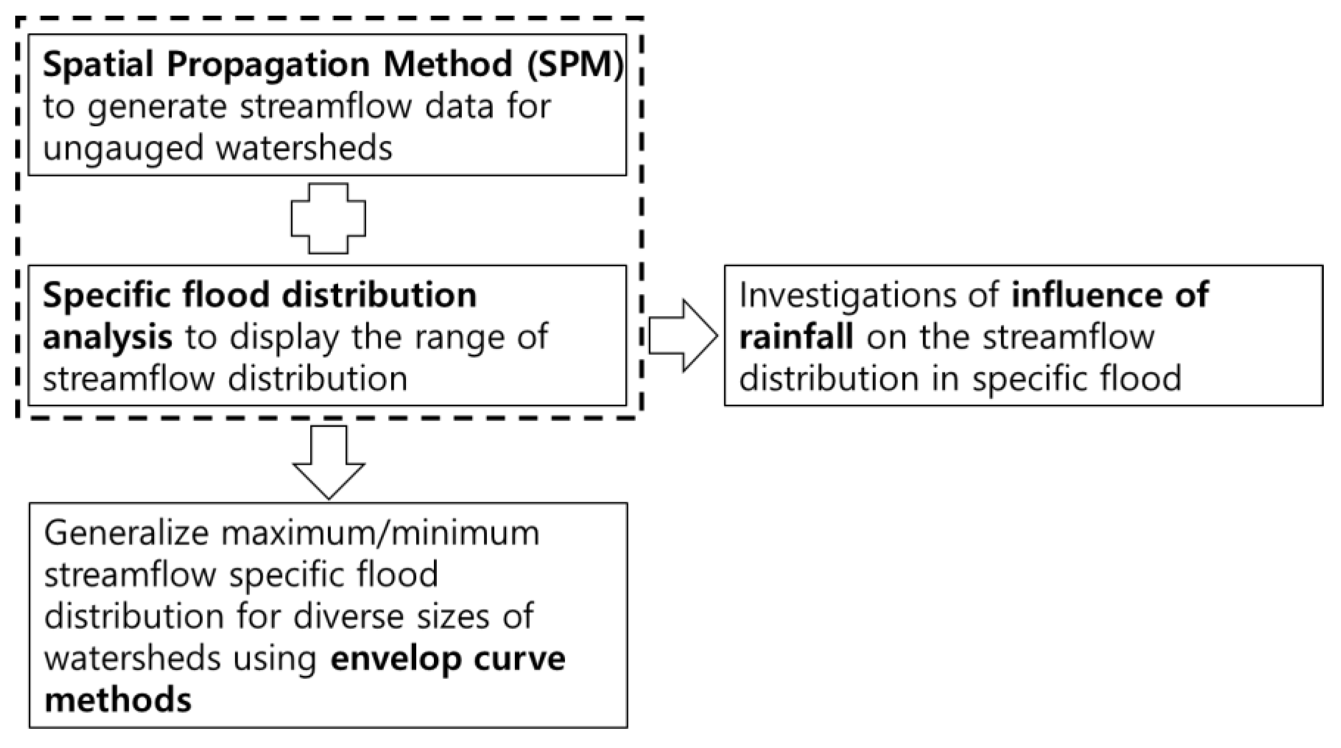
2. Methodology
3. Study Area and Storm Events
4. Results and Discussion
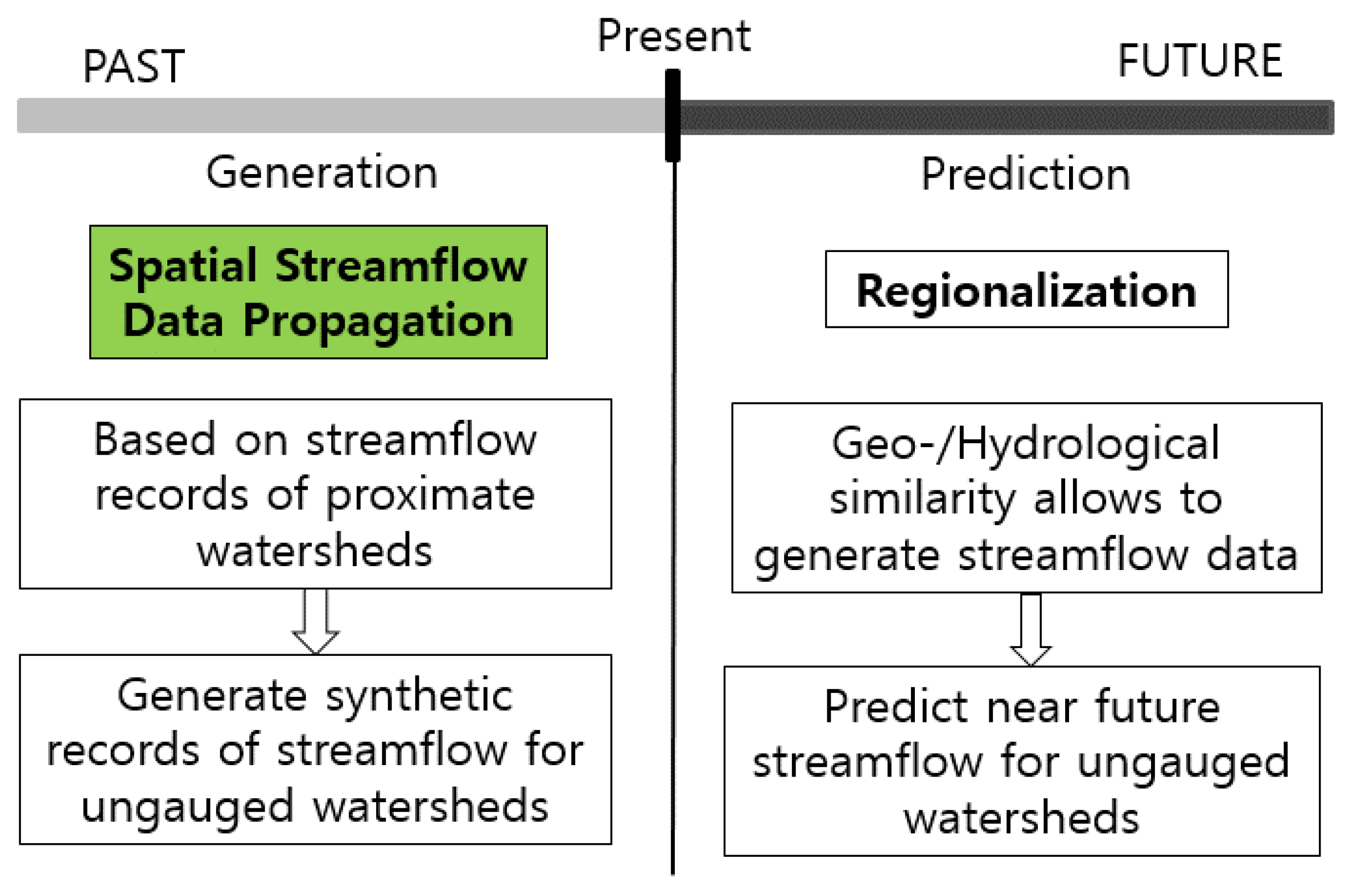
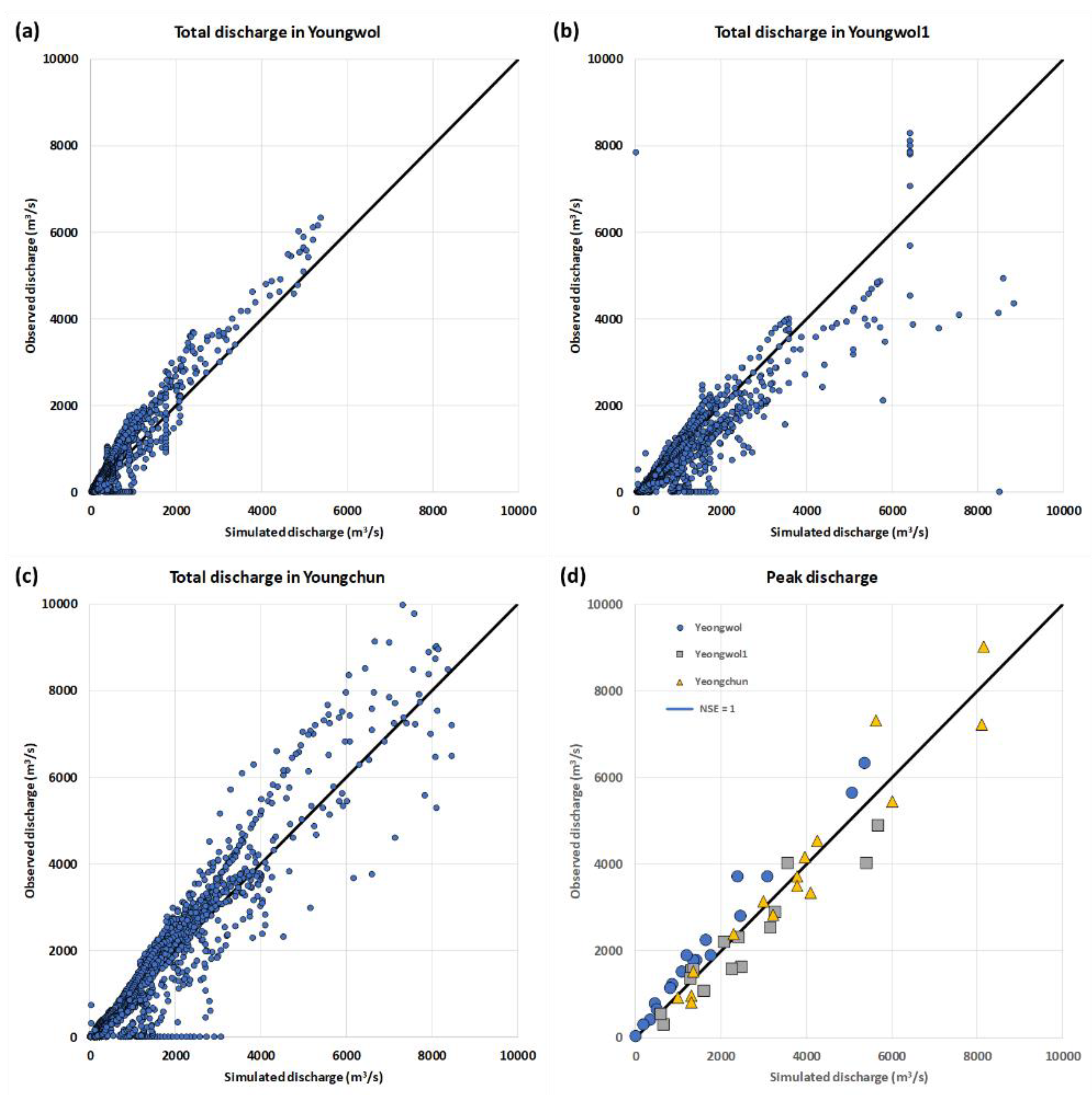
4.1. Generation of Streamflow Data
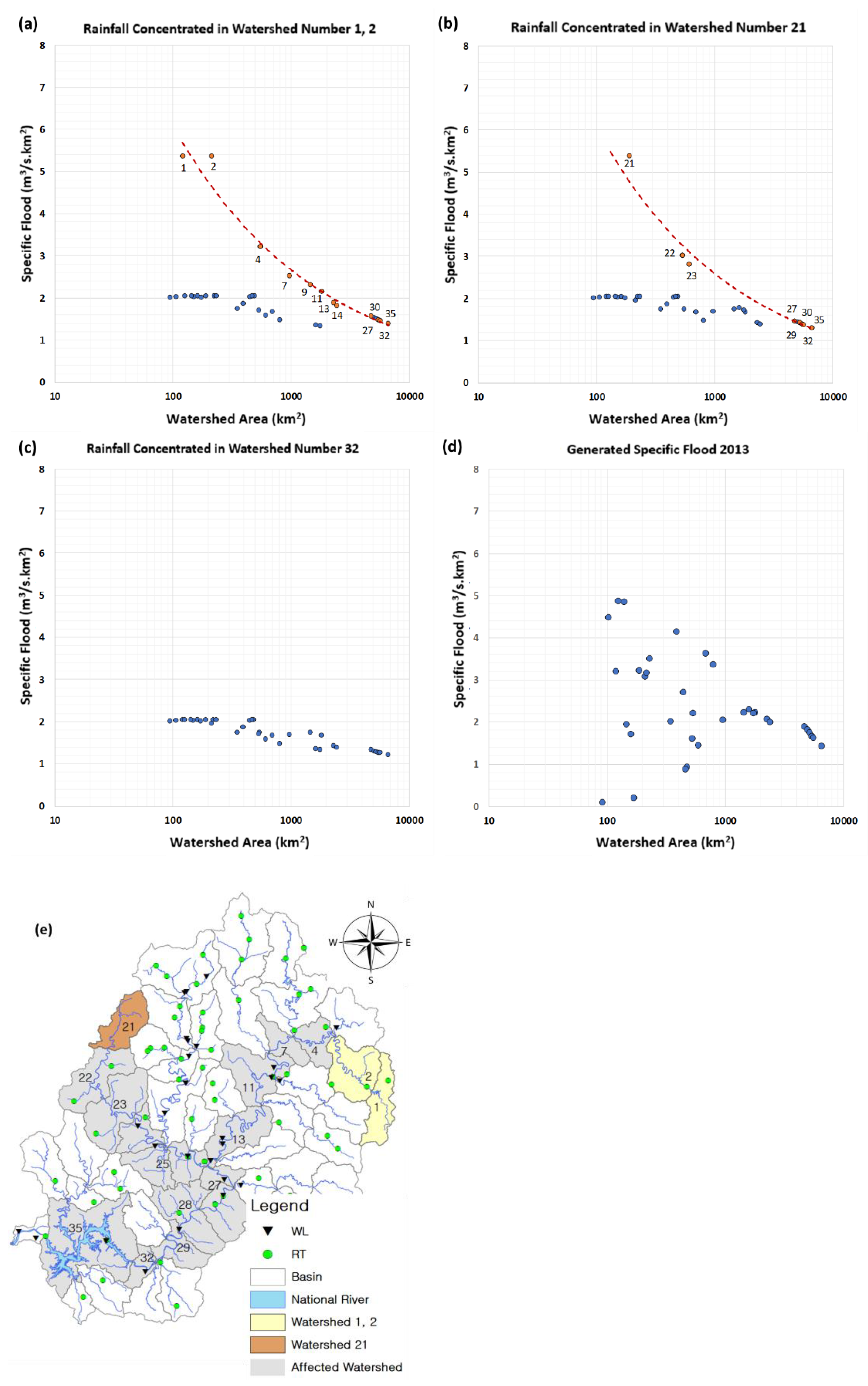
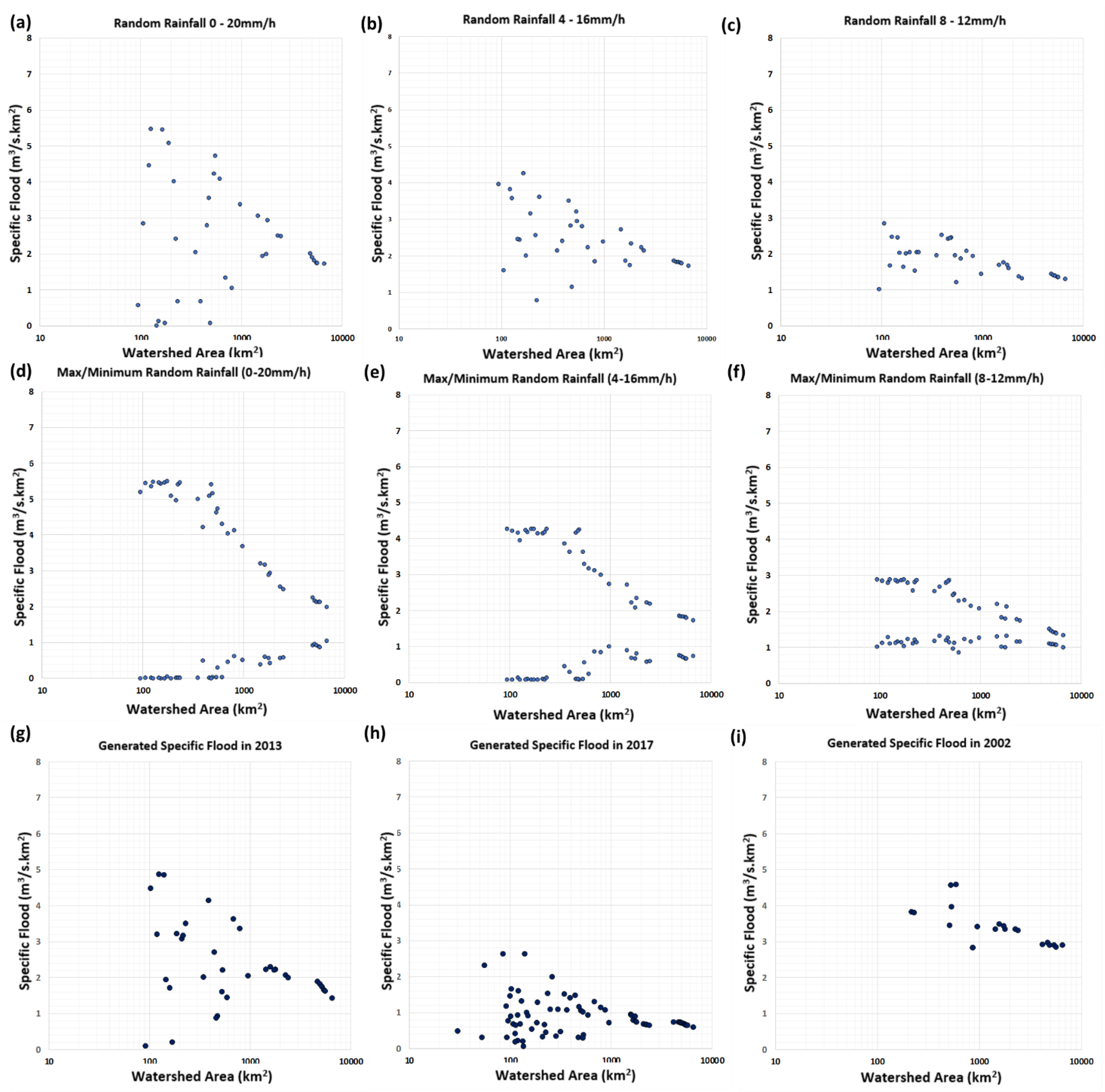
4.2. Effects of Rainfall on Specific Floods
4.2.1. Rainfall Locations
4.2.2. Rainfall Intensity and Duration
4.3. Ranges of Regional Floods
5. Conclusions
Author Contributions
Funding
Acknowledgments
Conflicts of Interest
References
- Pegram, G.; Parak, M. A review of the regional maximum flood and rational formula using geomorphological information and observed floods. Water SA 2004, 30, 377–392. [Google Scholar] [CrossRef] [Green Version]
- Kovacs, Z. Regional Maximum Flood Peaks in Southern Africa; Technical Report No. 137; Department of Water Affairs: Pretoria, South Africa, 1988. [Google Scholar]
- Acreman, M.C. Extreme historical UK Floods and maximum flood estimation. Water Environ. J. 1989, 3, 404–412. [Google Scholar] [CrossRef]
- Furey, P.R.; Gupta, V.K. Effects of excess rainfall on the temporal variability of observed peak-discharge power laws. Adv. Water Resour. 2005, 28, 1240–1253. [Google Scholar] [CrossRef]
- Furey, P.R.; Gupta, V.K. Diagnosing peak-discharge power laws observed in rainfall–runoff events in Goodwin Creek experimental watershed. Adv. Water Resour. 2007, 30, 2387–2399. [Google Scholar] [CrossRef]
- Patnaik, S.; Biswal, B.; Kumar, D.N.; Sivakumar, B. Effect of catchment characteristics on the relationship between past discharge and the power law recession coefficient. J. Hydrol. 2015, 528, 321–328. [Google Scholar] [CrossRef]
- Abdullah, J.; Muhammad, N.S.; Muhammad, S.A.; Julien, P.Y. Envelope curves for the specific discharge of extreme floods in Malaysia. J. Hydro-Environ. Res. 2019, 25, 1–11. [Google Scholar] [CrossRef]
- Sandrock, G.; Viraraghavan, T.; Fuller, G.A. Estimation of peak flows for natural ungauged watersheds in southern Saskatchewan. Can. Water Resour. J. 1992, 17, 21–31. [Google Scholar] [CrossRef]
- McDonnell, J.J.; Beven, K. Debates-The future of hydrological sciences: A (common) path forward? A call to action aimed at understanding velocities, celerities and residence time distributions of the headwater hydrograph. Water Resour. Res. 2014, 50, 5342–5350. [Google Scholar] [CrossRef]
- Merz, R.; Bloschl, G. Regionalisation of catchment model parameters. J. Hydrol. 2004, 287, 95–123. [Google Scholar] [CrossRef] [Green Version]
- Oudin, L.; Andréassian, V.C.; Perrin, C.; Michel, C.; Le Moine, N. Spatial proximity, physical similarity, regression and ungauged catchments: A comparison of regionalization approaches based on 913 French catchments. Water Resour. Res. 2008, 44, W03413. [Google Scholar] [CrossRef]
- Heřmanovský, M.; Havlíček, V.; Hanel, M.; Pech, P. Regionalization of runoff models derived by genetic programming. J. Hydrol. 2017, 547, 544–556. [Google Scholar] [CrossRef]
- Klotz, D.; Herrnegger, M.; Schulz, K. Symbolic Regression for the Estimation of Transfer Functions of Hydrological Models. Water Resour. Res. 2017, 53, 9402–9423. [Google Scholar] [CrossRef]
- Wagener, T.; Wheater, H.S. Parameter estimation and regionalization for continuous rainfall-runoff models including uncertainty. J. Hydrol. 2005, 320, 132–154. [Google Scholar] [CrossRef]
- Kim, N.W.; Jung, Y.; Lee, J.E. Spatial propagation of streamflow data in ungauged watersheds using a lumped conceptual model. J. Water Clim. Chang. 2019, 10, 89–101. [Google Scholar] [CrossRef] [Green Version]
- Ayalew, T.B.; Krajewski, W.F.; Mantilla, R.; Small, S.J. Exploring the effects of hillslope-channel link dynamics and excess rainfall properties on the scaling structure of peak-discharge. Adv. Water Resour. 2014, 64, 9–20. [Google Scholar] [CrossRef]
- Kimura, T. The Flood Runoff Analysis Method by the Storage Function Model; The Public Works of Research Institute, Ministry of Construction: Tokyo, Japan, 1961. [Google Scholar]
- Creager, W.P.; Justin, J.D.; Hinds, J. Engineering for Dams; General Design; John Wiley: New York, NY, USA, 1945; Volume 1. [Google Scholar]
- Ministry of Construction. Report of Water Resource Management in Korea: Guideline of Flood Design Estimation; Ministry of Construction: Seoul, Korea, 1993. [Google Scholar]
- Gupta, V.K.; Mantilla, R.; Troutman, B.M.; Dawdy, D.; Krajewski, W.F. Generalizing a nonlinear geophysical flood theory to medium-sized river networks. Geophys. Res. Lett. 2010, 37, 11402. [Google Scholar] [CrossRef]
- Lima, C.H.R.; Lall, U. Spatial scaling in a changing climate: A hierarchical Bayesian model for non-stationary multi-site annual maximum and monthly streamflow. J. Hydrol. 2010, 383, 307–318. [Google Scholar] [CrossRef]
- Smith, J.A.; Baeck, M.L.; Villarini, G.; Krajewski, W.F. The hydrology and hydrometeorology of flooding in the Delaware River basin. J. Hydrometeorol. 2010, 11, 841–859. [Google Scholar] [CrossRef]
- Mandapaka, P.V.; Krajewski, W.F.; Mantilla, R.; Gupta, V.K. Dissecting the effect of rainfall variability on the statistical structure of peak flows. Adv. Water Resour. 2009, 32, 1508–1525. [Google Scholar] [CrossRef]
- Bayazit, M.; Onoz, B. Envelope curve for maximum floods in Turkey. Digest 2004, 927–931. [Google Scholar]


| Event | Start | End | Total Rainfall (mm) | Event | Start | End | Total Rainfall (mm) |
|---|---|---|---|---|---|---|---|
| 1 | 2001/6/29 0:00 | 2001/7/4 0:00 | 101.88 | 10 | 2010/9/10 0:00 | 2010/9/15 0:00 | 150.33 |
| 2 | 2002/8/6 0:00 | 2002/8/10 0:00 | 375.94 | 11 | 2011/8/16 0:00 | 2011/8/19 0:00 | 145.78 |
| 3 | 2003/7/8 0:00 | 2003/7/13 0:00 | 79.86 | 12 | 2012/7/5 0:00 | 2012/7/8 0:00 | 184.17 |
| 4 | 2004/7/11 0:00 | 2004/7/15 0:00 | 136.64 | 13 | 2013/7/14 0:00 | 2013/7/17 0:00 | 163.16 |
| 5 | 2005/7/1 0:00 | 2005/7/3 0:00 | 102.42 | 14 | 2014/8/17 0:00 | 2014/8/23 0:00 | 106.44 |
| 6 | 2006/7/14 0:00 | 2006/7/20 0:00 | 441.94 | 15 | 2015/8/24 0:00 | 2015/8/29 0:00 | 53.65 |
| 7 | 2007/8/4 0:00 | 2007/8/7 0:00 | 126.01 | 16 | 2016/7/4 0:00 | 2016/7/8 0:00 | 227.03 |
| 8 | 2008/7/24 0:00 | 2008/7/29 0:00 | 197.40 | 17 | 2017/7/2 0:00 | 2017/7/6 0:00 | 190.55 |
| 9 | 2009/7/12 0:00 | 2009/7/14 0:00 | 142.90 | 18 | 2018/7/1 0:00 | 2018/7/5 0:00 | 136.79 |
Publisher’s Note: MDPI stays neutral with regard to jurisdictional claims in published maps and institutional affiliations. |
© 2021 by the authors. Licensee MDPI, Basel, Switzerland. This article is an open access article distributed under the terms and conditions of the Creative Commons Attribution (CC BY) license (https://creativecommons.org/licenses/by/4.0/).
Share and Cite
Kim, N.-W.; Kim, K.-H.; Jung, Y. Spatial Recognition of Regional Maximum Floods in Ungauged Watersheds and Investigations of the Influence of Rainfall. Atmosphere 2021, 12, 800. https://doi.org/10.3390/atmos12070800
Kim N-W, Kim K-H, Jung Y. Spatial Recognition of Regional Maximum Floods in Ungauged Watersheds and Investigations of the Influence of Rainfall. Atmosphere. 2021; 12(7):800. https://doi.org/10.3390/atmos12070800
Chicago/Turabian StyleKim, Nam-Won, Ki-Hyun Kim, and Yong Jung. 2021. "Spatial Recognition of Regional Maximum Floods in Ungauged Watersheds and Investigations of the Influence of Rainfall" Atmosphere 12, no. 7: 800. https://doi.org/10.3390/atmos12070800
APA StyleKim, N.-W., Kim, K.-H., & Jung, Y. (2021). Spatial Recognition of Regional Maximum Floods in Ungauged Watersheds and Investigations of the Influence of Rainfall. Atmosphere, 12(7), 800. https://doi.org/10.3390/atmos12070800