
How Much Building Renewable Energy Is Enough? The Vertical City Weather Generator (VCWG v1.4.4)


Abstract
:1. Introduction
1.1. Renewable and Alternative Energy Systems for Buildings
1.2. Renewable and Alternative Energy for Buildings in Cold Climates
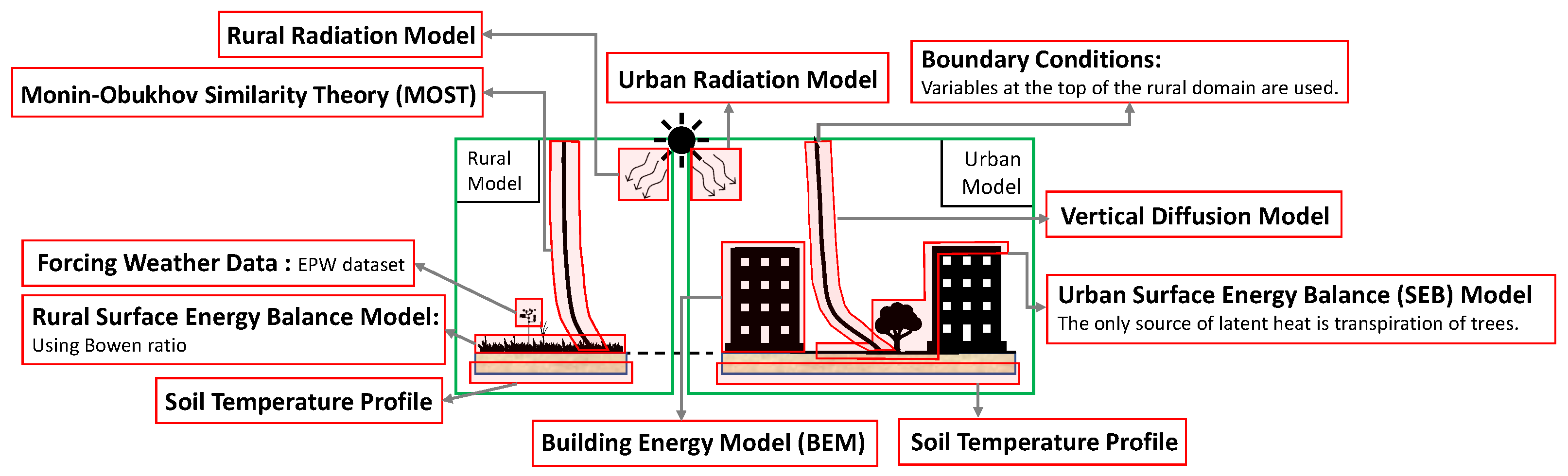
1.3. Building Performance Modeling by Feedback Interaction with Urban Climate-Weather Variables
1.4. Research Gaps and Objectives
2. Methodology
2.1. The Vertical City Weather Generator (VCWG)
2.2. Guelph Climate and the Urban Fabric
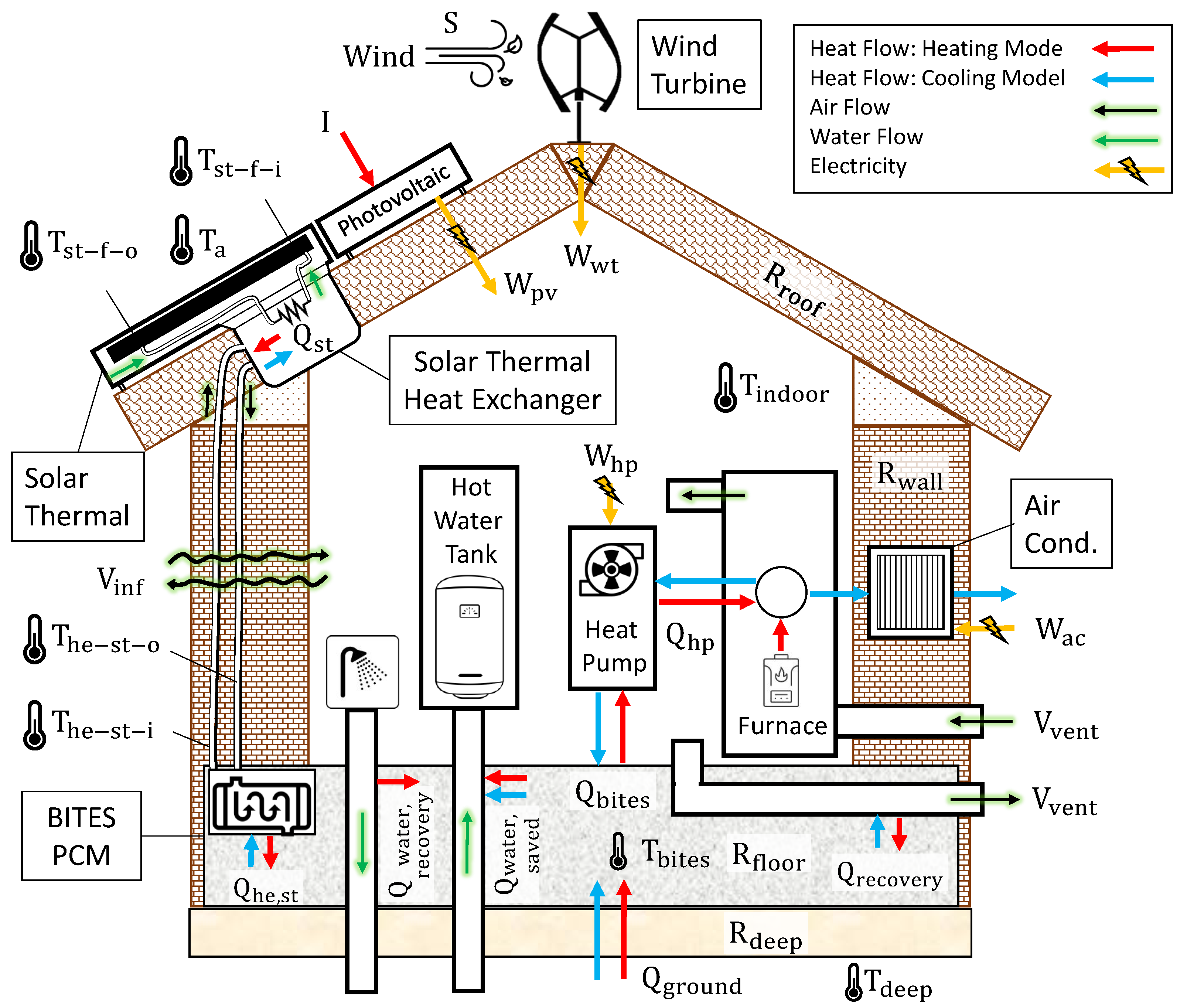
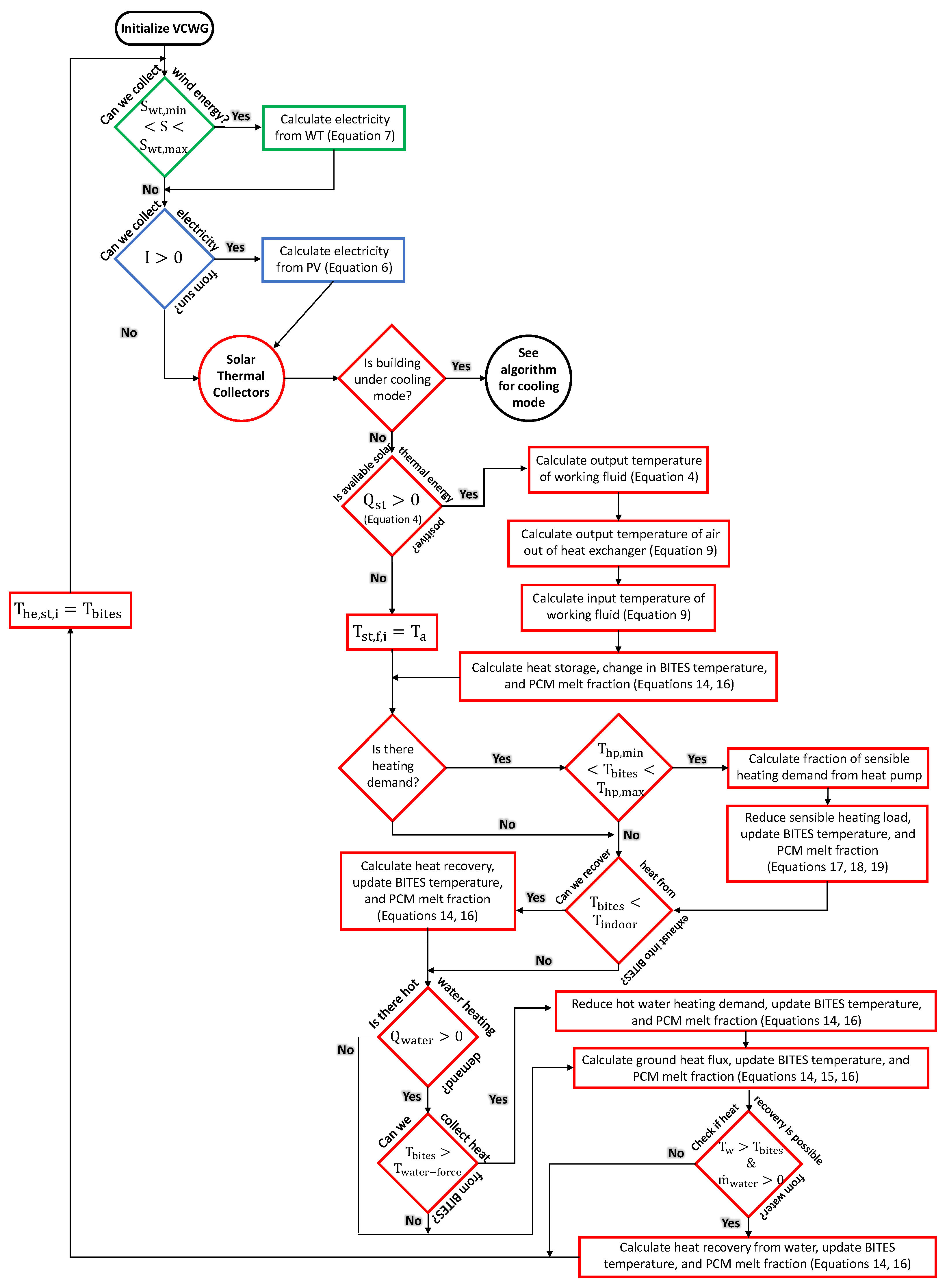
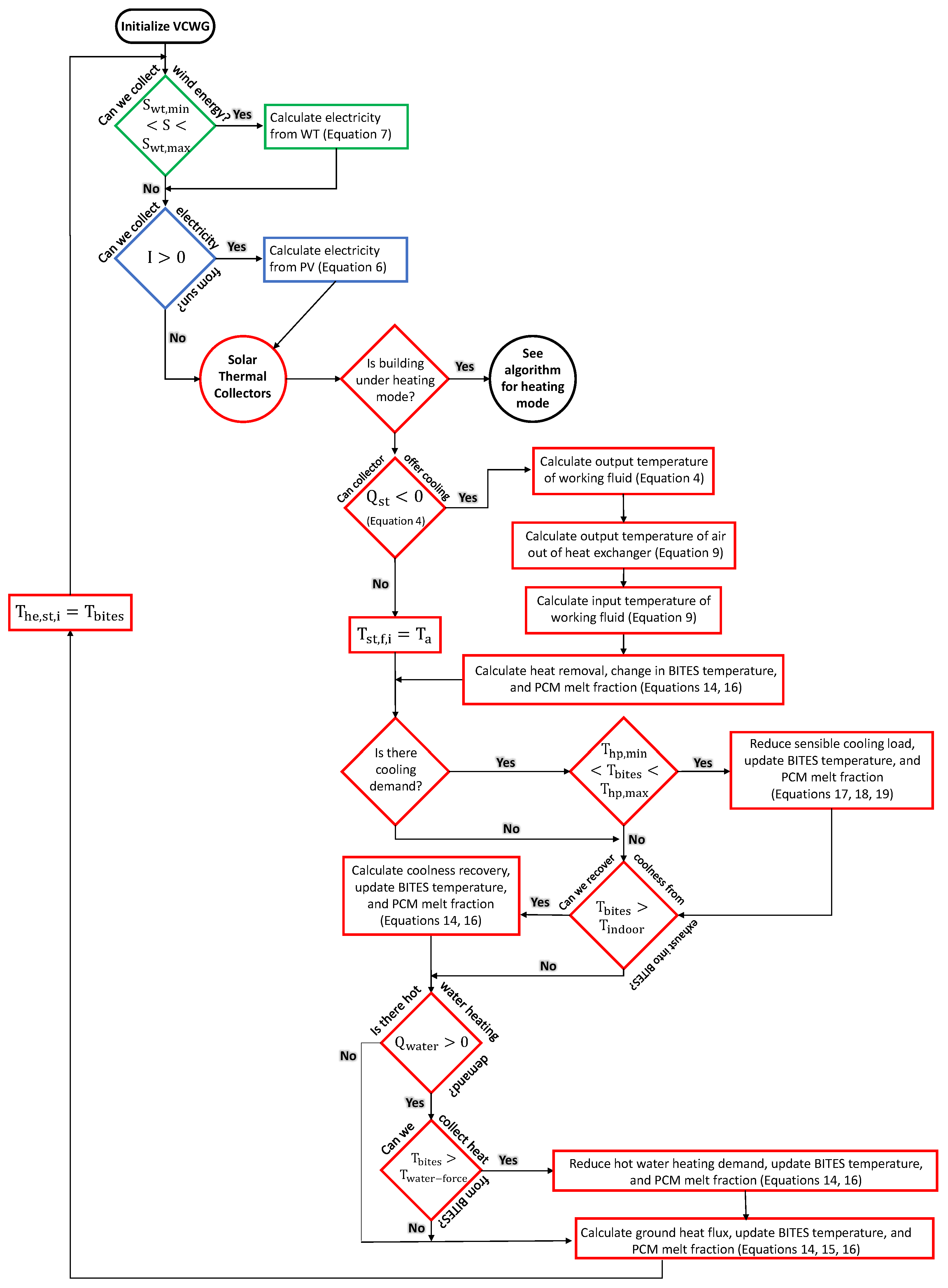
2.3. System Integration in VCWG v1.4.4
2.3.1. Solar Thermal Collectors
2.3.2. Photovoltaic Collectors
2.3.3. Wind Turbines
2.3.4. Heat Exchangers
2.3.5. Building Envelop
2.3.6. Thermal Energy Storage
2.3.7. Heat Pumps
2.4. Economic Assessment
2.5. System Optimization
3. Results and Discussion
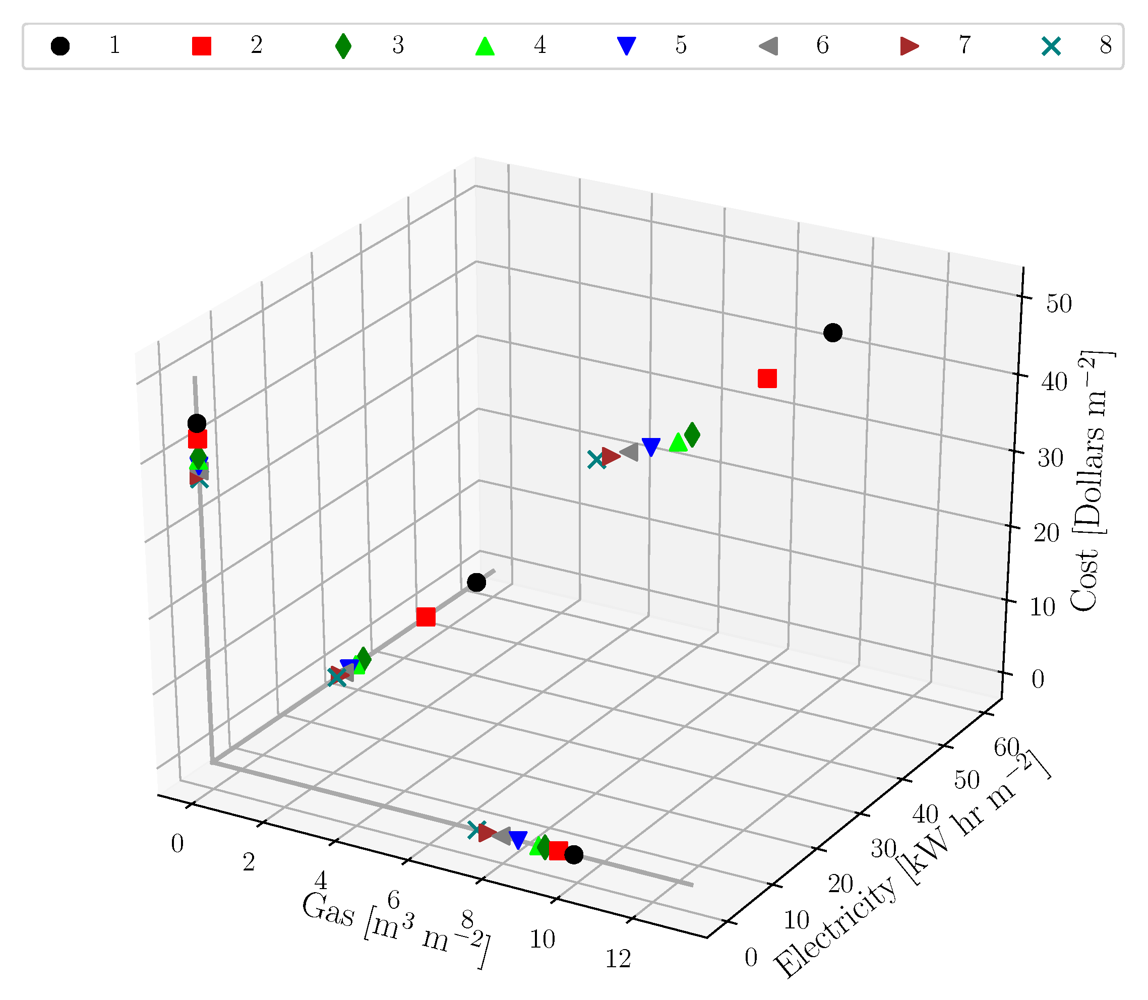
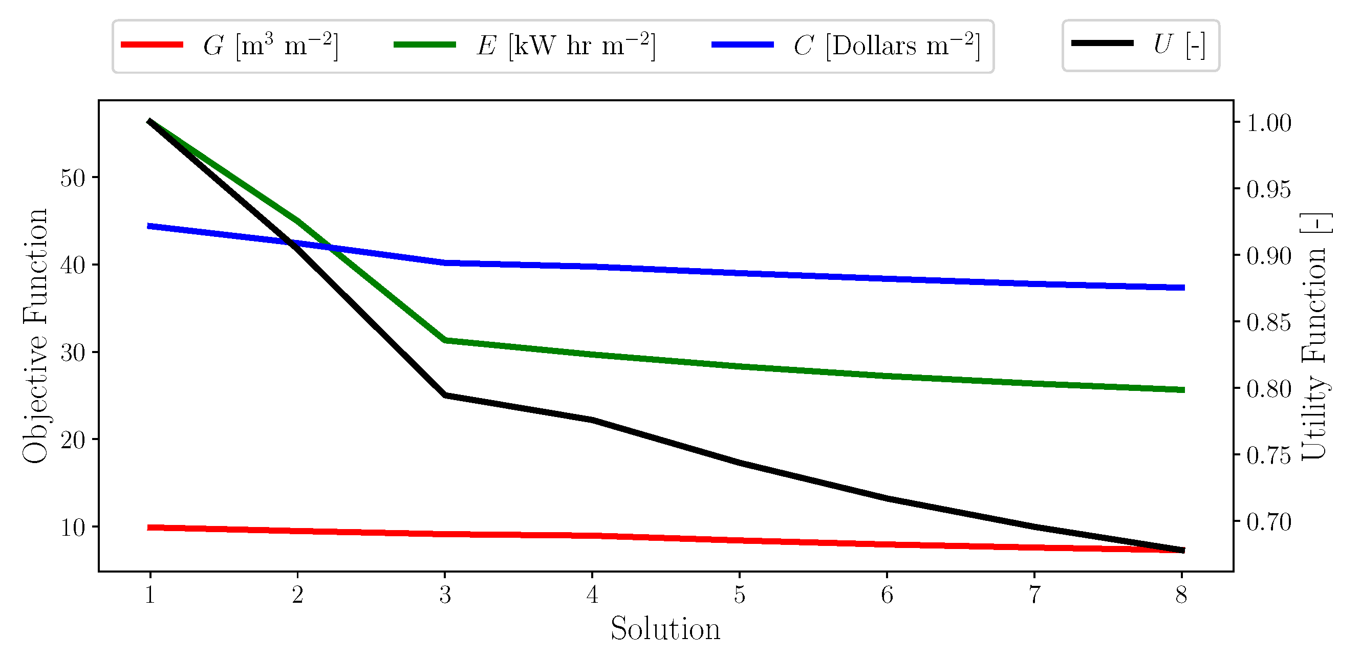
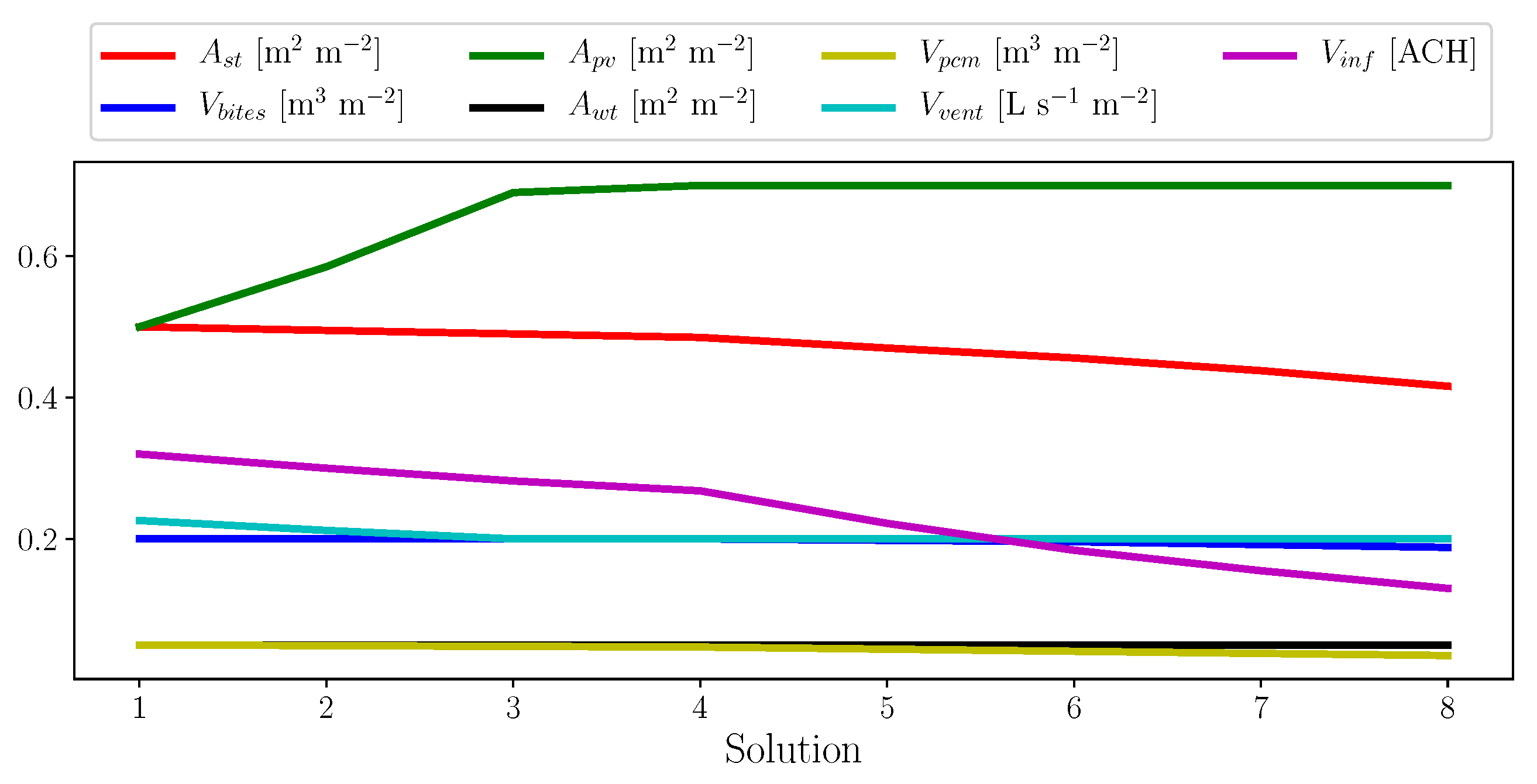
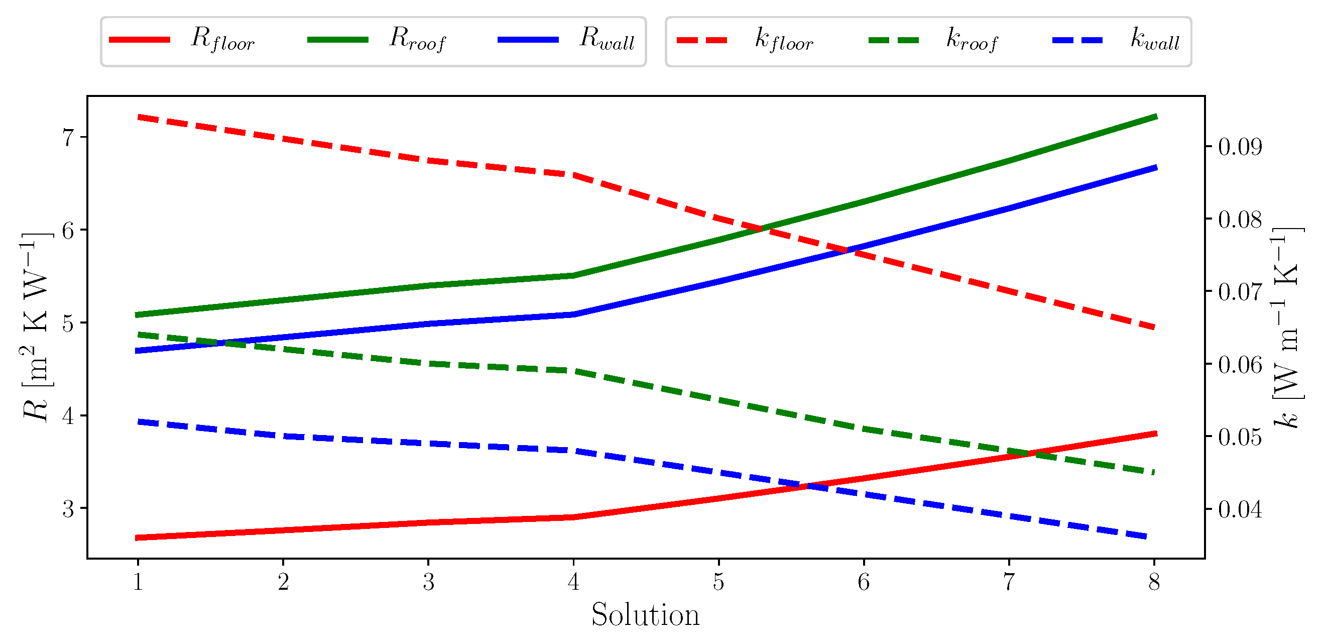
3.1. Annual Metrics and Optimization
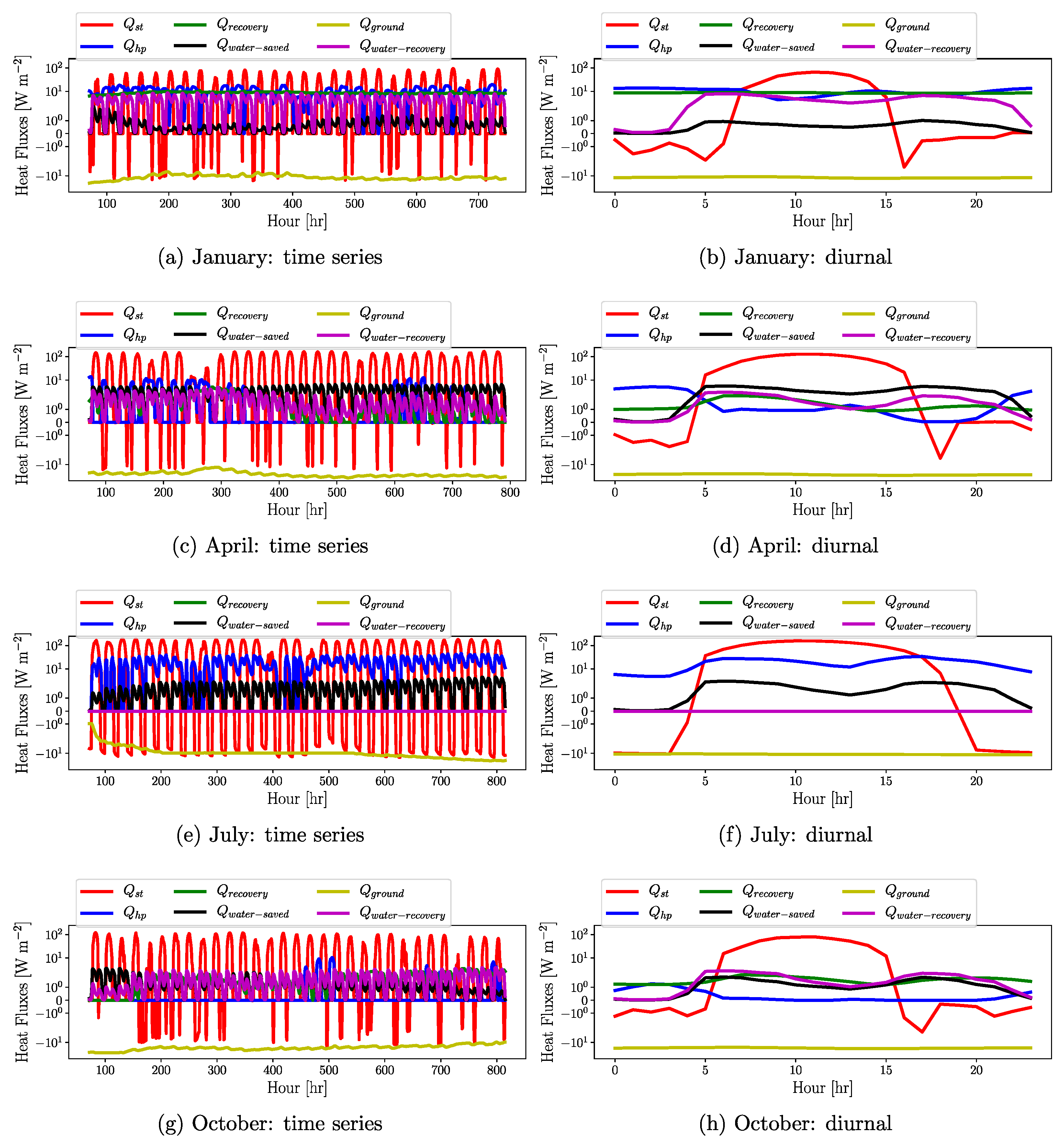
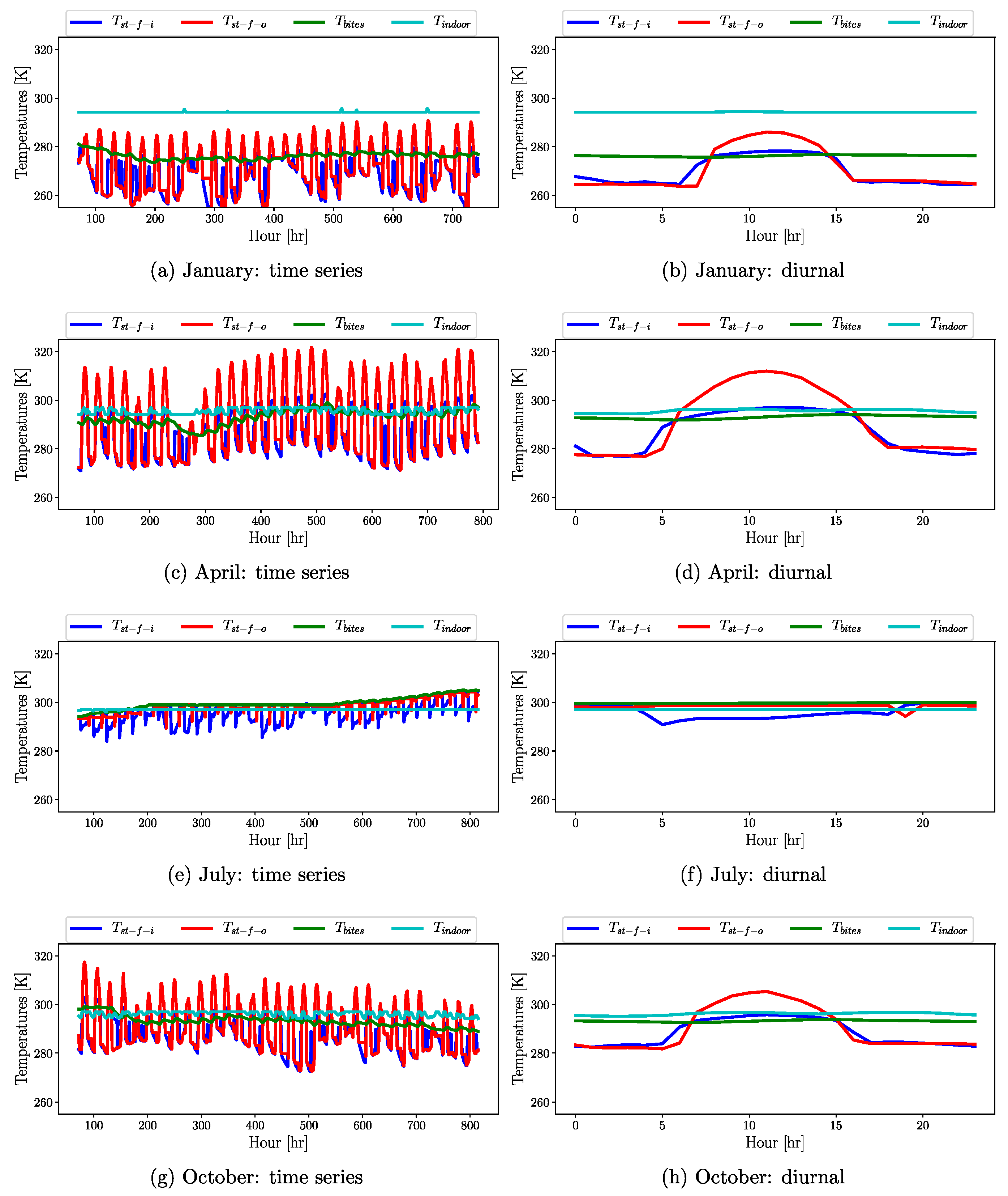
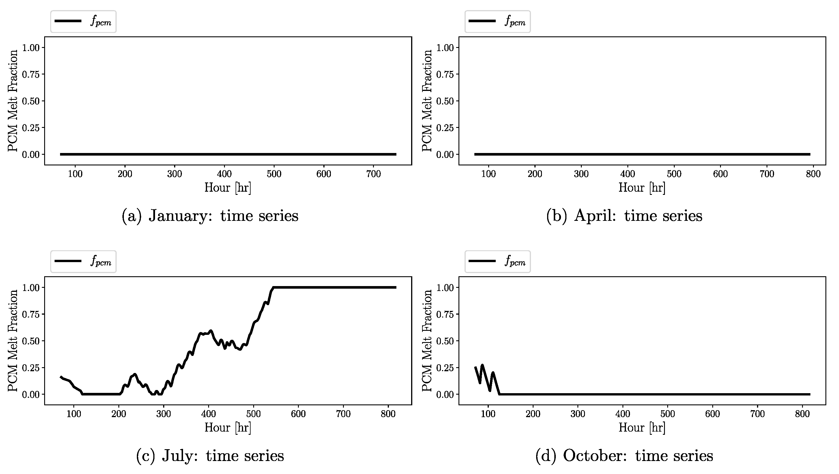
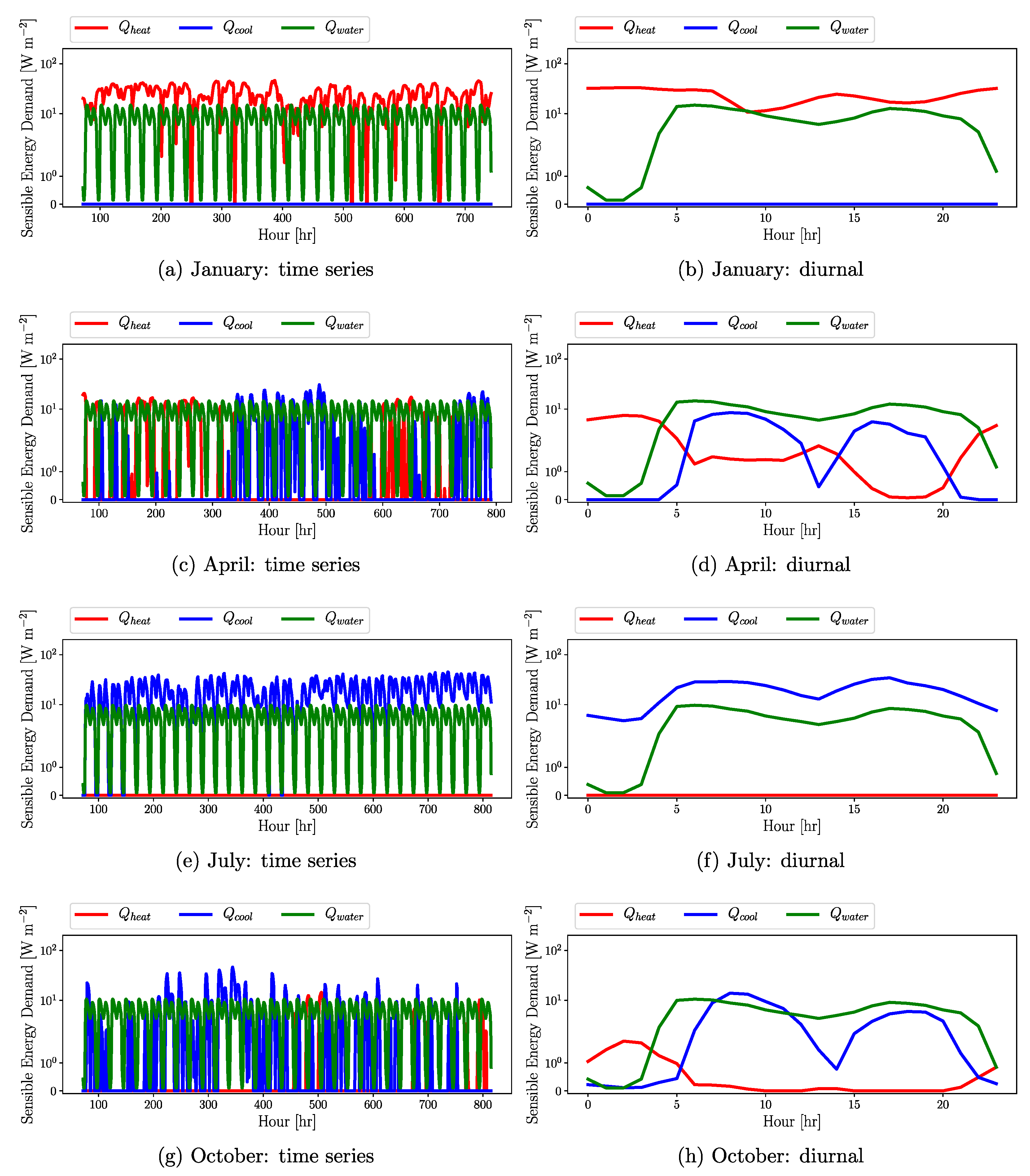
3.2. Seasonal and Diurnal Variation in Building Physical Variables
4. Conclusions and Future Work
Author Contributions
Funding
Institutional Review Board Statement
Informed Consent Statement
Data Availability Statement
Acknowledgments
Conflicts of Interest
Appendix A


References
- Kim, G.; Lim, H.S.; Lim, T.S.; Schaefer, L.; Kim, J.T. Comparative advantage of an exterior shading device in thermal performance for residential buildings. Energy Build. 2012, 46, 105–111. [Google Scholar] [CrossRef]
- Bilardo, M.; Ferrara, M.; Fabrizio, E. Performance assessment and optimization of a solar cooling system to satisfy renewable energy ratio (RER) requirements in multi-family buildings. Renew. Energy 2020, 155, 990–1008. [Google Scholar] [CrossRef]
- Khan, M.M.A.; Ibrahim, N.I.; Mahbubul, I.; Muhammad. Ali, H.; Saidur, R.; Al-Sulaiman, F.A. Evaluation of solar collector designs with integrated latent heat thermal energy storage: A review. Sol. Energy 2018, 166, 334–350. [Google Scholar] [CrossRef]
- Zhang, X.; Shen, J.; Lu, Y.; He, W.; Xu, P.; Zhao, X.; Qiu, Z.; Zhu, Z.; Zhou, J.; Dong, X. Active Solar Thermal Facades (ASTFs): From concept, application to research questions. Renew. Sustain. Energy Rev. 2015, 50, 32–63. [Google Scholar] [CrossRef]
- Maurer, C.; Cappel, C.; Kuhn, T.E. Progress in building-integrated solar thermal systems. Sol. Energy 2017, 154, 158–186. [Google Scholar] [CrossRef]
- Al-Waeli, A.H.; Sopian, K.; Kazem, H.A.; Chaichan, M.T. Nanofluid based grid connected PV/T systems in Malaysia: A techno-economical assessment. Sustain. Energy Technol. Assess. 2018, 28, 81–95. [Google Scholar] [CrossRef]
- Kośny, J.; Biswas, K.; Miller, W.; Kriner, S. Field thermal performance of naturally ventilated solar roof with PCM heat sink. Sol. Energy 2012, 86, 2504–2514. [Google Scholar] [CrossRef]
- Navarro, L.; de Gracia, A.; Niall, D.; Castell, A.; Browne, M.; McCormack, S.J.; Griffiths, P.; Cabeza, L.F. Thermal energy storage in building integrated thermal systems: A review. Part 2. Integration as passive system. Renew. Energy 2016, 85, 1334–1356. [Google Scholar] [CrossRef] [Green Version]
- Navarro, L.; de Gracia, A.; Colclough, S.; Browne, M.; McCormack, S.J.; Griffiths, P.; Cabeza, L.F. Thermal energy storage in building integrated thermal systems: A review. Part 1. active storage systems. Renew. Energy 2016, 88, 526–547. [Google Scholar] [CrossRef] [Green Version]
- Olsthoorn, D.; Haghighat, F.; Moreau, A.; Lacroix, G. Abilities and limitations of thermal mass activation for thermal comfort, peak shifting and shaving: A review. Build. Environ. 2017, 118, 113–127. [Google Scholar] [CrossRef]
- de Gracia, A.; Cabeza, L.F. Phase change materials and thermal energy storage for buildings. Energy Build. 2015, 103, 414–419. [Google Scholar] [CrossRef] [Green Version]
- Ekrami, N.; Garat, A.; Fung, A.S. Thermal Analysis of Insulated Concrete Form (ICF) Walls. Energy Procedia 2015, 75, 2150–2156. [Google Scholar] [CrossRef] [Green Version]
- Faraj, K.; Khaled, M.; Faraj, J.; Hachem, F.; Castelain, C. Phase change material thermal energy storage systems for cooling applications in buildings: A review. Renew. Sustain. Energy Rev. 2020, 119, 109579. [Google Scholar] [CrossRef]
- Kalidasan, B.; Pandey, A.K.; Shahabuddin, S.; Samykano, M.; Thirugnanasambandam, M.; Saidur, R. Phase change materials integrated solar thermal energy systems: Global trends and current practices in experimental approaches. J. Energy Storage 2020, 27, 101118. [Google Scholar] [CrossRef]
- Jin, X.; Zhang, X. Thermal analysis of a double layer phase change material floor. Appl. Therm. Eng. 2011, 31, 1576–1581. [Google Scholar] [CrossRef]
- Pomianowski, M.; Heiselberg, P.; Jensen, R.L. Dynamic heat storage and cooling capacity of a concrete deck with PCM and thermally activated building system. Energy Build. 2012, 53, 96–107. [Google Scholar] [CrossRef]
- Wardziak, L.; Jaworski, M. Computer simulations of heat transfer in a building integrated heat storage unit made of PCM composite. Therm. Sci. Eng. Prog. 2017, 2, 109–118. [Google Scholar] [CrossRef]
- Bland, A.; Khzouz, M.; Statheros, T.; Gkanas, E.I. PCMs for Residential Building Applications: A Short Review Focused on Disadvantages and Proposals for Future Development. Buildings 2017, 7, 78. [Google Scholar] [CrossRef] [Green Version]
- Javadi, F.; Metselaar, H.; Ganesan, P. Performance improvement of solar thermal systems integrated with phase change materials (PCM), a review. Sol. Energy 2020, 206, 330–352. [Google Scholar] [CrossRef]
- Kapsalis, V.; Karamanis, D. Solar thermal energy storage and heat pumps with phase change materials. Appl. Therm. Eng. 2016, 99, 1212–1224. [Google Scholar] [CrossRef]
- NRCan. Heating and Cooling with a Heat Pump; Technical Report; Office of Energy Efficiency, Natural Resources Canada: Gatineau, QC, Canada, 2004. [Google Scholar]
- Chen, Y.; Athienitis, A.K.; Galal, K. Modeling, design and thermal performance of a BIPV/T system thermally coupled with a ventilated concrete slab in a low energy solar house: Part 1, BIPV/T system and house energy concept. Sol. Energy 2010, 84, 1892–1907. [Google Scholar] [CrossRef]
- Chen, Y.; Galal, K.; Athienitis, A.K. Modeling, design and thermal performance of a BIPV/T system thermally coupled with a ventilated concrete slab in a low energy solar house: Part 2, ventilated concrete slab. Sol. Energy 2010, 84, 1908–1919. [Google Scholar] [CrossRef]
- Fraisse, G.; Johannes, K.; Trillat-Berdal, V.; Achard, G. The use of a heavy internal wall with a ventilated air gap to store solar energy and improve summer comfort in timber frame houses. Energy Build. 2006, 38, 293–302. [Google Scholar] [CrossRef]
- Kamel, R.; Ekrami, N.; Dash, P.; Fung, A.; Hailu, G. BIPV/T + ASHP: Technologies for NZEBs. Energy Procedia 2015, 78, 424–429. [Google Scholar] [CrossRef] [Green Version]
- Tardif, J.M.; Tamasauskas, J.; Delisle, V.; Kegel, M. Performance of Air Based BIPV/T Heat Management Strategies in a Canadian Home. Procedia Environ. Sci. 2017, 38, 140–147. [Google Scholar] [CrossRef]
- Fallahi, A.; Haghighat, F.; Elsadi, H. Energy performance assessment of double-skin façade with thermal mass. Energy Build. 2010, 42, 1499–1509. [Google Scholar] [CrossRef]
- Harish, V.; Kumar, A. A review on modeling and simulation of building energy systems. Renew. Sustain. Energy Rev. 2016, 56, 1272–1292. [Google Scholar] [CrossRef]
- Connolly, D.; Lund, H.; Mathiesen, B.; Leahy, M. A review of computer tools for analysing the integration of renewable energy into various energy systems. Appl. Energy 2010, 87, 1059–1082. [Google Scholar] [CrossRef]
- Mills, G. An urban canopy-layer climate model. Theor. Appl. Climatol. 1997, 57, 229–244. [Google Scholar] [CrossRef]
- Kusaka, H.; Kondo, H.; Kikegawa, Y.; Kimura, F. A simple single-layer urban canopy model for atmospheric models: Comparison with multi-layer and slab models. Bound. Layer Meteorol. 2001, 101, 329–358. [Google Scholar] [CrossRef]
- Salamanca, F.; Krpo, A.; Martilli, A.; Clappier, A. A new building energy model coupled with an urban canopy parameterization for urban climate simulations–part I. formulation, verification, and sensitivity analysis of the model. Theor. Appl. Climatol. 2010, 99, 331–344. [Google Scholar] [CrossRef]
- Ryu, Y.H.; Baik, J.J.; Lee, S.H. A new single-layer urban canopy model for use in mesoscale atmospheric models. J. Appl. Meteorol. Clim. 2011, 50, 1773–1794. [Google Scholar] [CrossRef]
- Bueno Unzeta, B. An Urban Weather Generator Coupling a Building Simulation Program with an Urban Canopy Model. Master’s Thesis, Massachusetts Institute of Technology, Cambridge, MA, USA, 2010. [Google Scholar]
- Bueno, B.; Norford, L.K.; Pigeon, G.; Britter, R. Combining a detailed building energy model with a physically-based urban canopy model. Bound. Layer Meteorol. 2011, 140, 471–489. [Google Scholar] [CrossRef]
- Bueno, B.; Norford, L.; Hidalgo, J.; Pigeon, G. The urban weather generator. J. Build. Perf. Simulat. 2012, 6, 269–281. [Google Scholar] [CrossRef]
- Bueno, B.; Pigeon, G.; Norford, L.K.; Zibouche, K.; Marchadier, C. Development and evaluation of a building energy model integrated in the TEB scheme. Geosci. Model Dev. 2012, 5, 433–448. [Google Scholar] [CrossRef] [Green Version]
- Bueno, B.; Roth, M.; Norford, L.K.; Li, R. Computationally efficient prediction of canopy level urban air temperature at the neighbourhood scale. Urban Clim. 2014, 9, 35–53. [Google Scholar] [CrossRef] [Green Version]
- Moradi, M.; Dyer, B.; Nazem, A.; Nambiar, M.K.; Nahian, M.R.; Bueno, B.; Mackey, C.; Vasanthakumar, S.; Nazarian, N.; Krayenhoff, E.S.; et al. The Vertical City Weather Generator (VCWG v1.3.2). Geosci. Model Dev. 2021, 14, 961–984. [Google Scholar] [CrossRef]
- Krayenhoff, E.S.; Voogt, J.A. A microscale three-dimensional urban energy balance model for studying surface temperatures. Bound. Layer Meteorol. 2007, 123, 433–461. [Google Scholar] [CrossRef]
- Yaghoobian, N.; Kleissl, J. Effect of reflective pavements on building energy use. Urban Clim. 2012, 2, 25–42. [Google Scholar] [CrossRef] [Green Version]
- Martilli, A.; Clappier, A.; Rotach, M.W. An urban surface exchange parameterisation for mesoscale models. Bound. Layer Meteorol. 2002, 104, 261–304. [Google Scholar] [CrossRef]
- Krayenhoff, E.S. A Multi-Layer Urban Canopy Model for Neighbourhoods with Trees. Ph.D. Thesis, University of British Columbia, Vancouver, BC, Canada, 2014. [Google Scholar] [CrossRef]
- Krayenhoff, E.S.; Jiang, T.; Christen, A.; Martilli, A.; Oke, T.R.; Bailey, B.N.; Nazarian, N.; Voogt, J.A.; Giometto, M.G.; Stastny, A.; et al. A multi-layer urban canopy meteorological model with trees (BEP-Tree): Street tree impacts on pedestrian-level climate. Urban Clim. 2020, 32, 100590. [Google Scholar] [CrossRef]
- Bueno Unzeta, B. Study and Prediction of the Energy Interactions between Buildings and the Urban Climate. Ph.D. Thesis, Massachusetts Institute of Technology, Cambridge, MA, USA, 2012. [Google Scholar]
- Aliabadi, A.A.; Moradi, M.; Clement, D.; Lubitz, W.D.; Gharabaghi, B. Flow and temperature dynamics in an urban canyon under a comprehensive set of wind directions, wind speeds, and thermal stability conditions. Environ. Fluid Mech. 2019, 19, 81–109. [Google Scholar] [CrossRef]
- Aliabadi, A.A.; Moradi, M.; Byerlay, R.A.E. The budgets of turbulence kinetic energy and heat in the urban roughness sublayer. Environ. Fluid Mech. 2021. [Google Scholar] [CrossRef]
- Smith, C.C.; Weiss, T.A. Design application of the Hottel-Whillier-Bliss equation. Sol. Energy 1977, 19, 109–113. [Google Scholar] [CrossRef] [Green Version]
- Aliabadi, A.A.; Wallace, J.S. Cost-effective and Reliable Design of a Solar Thermal Power Plant. Trans. Can. Soc. Mech. Eng. 2009, 33, 25–37. [Google Scholar] [CrossRef]
- Dongre, B.; Pateriya, R.K. Power curve model classification to estimate wind turbine power output. Wind Eng. 2019, 43, 213–224. [Google Scholar] [CrossRef]
- Bergia Boccardo, L.; Kazanci, O.B.; Quesada Allerhand, J.; Olesen, B.W. Economic comparison of TABS, PCM ceiling panels and all-air systems for cooling offices. Energy Build. 2019, 205, 109527. [Google Scholar] [CrossRef]
- Fu, R.; Margolis, R.; Woodhouse, M.; Ardani, K. U.S. Solar Photovoltaic System Cost Benchmark: Q1 2017; Technical Report; National Renewable Energy Laboratory (NREL): Washington, DC, USA, 2017.
- Marler, R.T.; Arora, J.S. The weighted sum method for multi-objective optimization: New insights. Struct. Multidisc. Optim. 2010, 41, 853–862. [Google Scholar] [CrossRef]
- Aliabadi, A.A.; Krayenhoff, E.S.; Nazarian, N.; Chew, L.W.; Armstrong, P.R.; Afshari, A.; Norford, L.K. Effects of roof-edge roughness on air temperature and pollutant concentration in urban canyons. Bound. Layer Meteorol. 2017, 164, 249–279. [Google Scholar] [CrossRef]


| Parameter | Symbol | Value |
|---|---|---|
| Latitude [°N] | lat | 43.524 |
| Longitude [°W] | lon | 80.104 |
| Average buildings height [m] | 6 | |
| Width of canyon [m] | 23 | |
| Building width to canyon width ratio [-] | 0.42 | |
| Leaf Area Index [m m] | 0–1 | |
| Tree height [m] | 3.5 | |
| Tree crown radius [m] | 1.5 | |
| Tree distance from wall [m] | 2.2 | |
| Ground vegetation cover fraction | 0.5 | |
| Building type | - | Mid rise apartment |
| Urban albedos (roof, ground, wall, vegetation) | 0.22, 0.1, 0.4, 0.2 | |
| Urban emissivities (roof, ground, wall, vegetation) | 0.95, 0.95, 0.95, 0.95 | |
| Rural overall albedo | 0.2 | |
| Rural overall emissivity | 0.95 | |
| Rural aerodynamic roughness length [m] | 0.2 | |
| Rural roughness length for temperature [m] | 0.02 | |
| Rural roughness length for specific humidity [m] | 0.02 | |
| Rural zero displacement height [m] | 1 | |
| Rural Bown ratio [-] | 1.5 | |
| Ground aerodynamic roughness length [m] | 0.02 | |
| Roof aerodynamic roughness length [m] | 0.02 | |
| Vertical resolution [m] | 1 | |
| Time step [s] | 60 | |
| Canyon axis orientation [°N] | 45 |
| Parameter | Units | Value | Description |
|---|---|---|---|
| [] | 43.67 | ST tilt angle | |
| [m m] | 0.5 | Area of ST per building footprint area | |
| [W m K] | 3 | Loss coefficient of ST | |
| [-] | 0.9 | Heat removal factor of ST | |
| [-] | 0.7 | Effective transmittance-absorptance of ST | |
| [-] | 0.8 | Heat exchange efficiency of ST (fluid to air) | |
| [m m] | 0.2 | Volume of BITES per building footprint area | |
| [J m K] | 5,244,160 | Volumetric heat capacity of BITES | |
| [kg s m] | 0.002 | Mass flow rate of working fluid in ST | |
| [J kg K] | 4200 | Heat capacity of working fluid in ST | |
| [kg s m] | 0.002 | Mass flow rate of air in ST heat exchanger | |
| [] | 43.67 | PV tilt angle | |
| [m m] | 0.5 | Area of PV per building footprint area | |
| [-] | 0.17 | Electrical efficiency of PV | |
| [-] | 1.5 | Minimum of auxiliary HP at minimum temperature | |
| [-] | 4 | Maximum of auxiliary HP at maximum temperature | |
| [K] | 253.15 | Minimum Temperature of auxiliary HP | |
| [K] | 308.15 | Maximum Temperature of auxiliary HP | |
| [m m] | 0.05 | Swept area of WT per building footprint area | |
| [-] | 0.4 | Electrical efficiency of WT | |
| [m s] | 2 | Minimum wind speed for WT | |
| [m s] | 15 | Maximum wind speed for WT | |
| [m m] | 0.05 | Volume of PCM per building footprint area (not zero) | |
| [J m] | 201,600,000 | Volumetric latent heat of PCM | |
| [K] | 299 | Melting temperature of PCM | |
| [L s m] | 0.226 | Ventilation rate per floor area | |
| [ACH] | 0.32 | Infiltration rate | |
| [m K W] | 4.696 | Thermal resistance of wall | |
| [W m K] | 0.052 | Thermal conductivity of wall | |
| [J m K] | 289,011 | Volumetric heat capacity of wall | |
| [m K W] | 5.083 | Thermal resistance of roof | |
| [W m K] | 0.064 | Thermal conductivity of roof | |
| [J m K] | 195,080 | Volumetric heat capacity of roof | |
| [m K W] | 2.680 | Thermal resistance of floor | |
| [W m K] | 0.0942 | Thermal conductivity of floor | |
| [J m K] | 1,258,814 | Volumetric heat capacity of floor | |
| [-] | 0.95 | Thermal efficiency of furnace and water heater |
| Layer | Layer Name | Thickness [m] | Conductivity [W m K] | Density [kg m] | Heat Capacity [J kg K] | Resistance [m K W] | Vapor Res. [GN s kg m] | Category |
|---|---|---|---|---|---|---|---|---|
| External Wall | ||||||||
| 1 | Rain screen | 0.0030 | 50.000 | 7800 | 450 | 0.00006 | −1.00f | Metal |
| 2 | Cavity | 0.0500 | 0.13000 | |||||
| 3 | EPP | 0.1651 | 00.039 | 60 | 1800 | 4.23330 | −1.00f | Insulation |
| 4 | Chipboard | 0.0111 | 00.150 | 800 | 2093 | 0.07400 | 450.00f | Timber |
| 5 | Gypsum | 0.0127 | 00.160 | 801 | 837 | 0.07940 | 45.00f | Plaster |
| 6 | Inside surface | 0.11700 | ||||||
| 7 | Outside surface | 0.06000 | ||||||
| Total | 0.2419 | 00.052 | 4.69400 | |||||
| Roof | ||||||||
| 1 | Asphalt | 0.0127 | 00.500 | 1700 | 1000 | 0.02540 | 5000.00f | Asphalt |
| 2 | Plywood | 0.0127 | 00.130 | 500 | 1500 | 0.09770 | −1.00f | Timber |
| 3 | EPP | 0.0825 | 00.039 | 60 | 1800 | 2.11540 | −1.00f | Insulation |
| 4 | Plywood | 0.0127 | 00.130 | 500 | 1500 | 0.09770 | −1.00f | Timber |
| 5 | Batt insulation | 0.1905 | 00.076 | 32 | 837 | 2.5099 | 7.00f | Insulation |
| 5 | Gypsum | 0.0127 | 00.160 | 801 | 837 | 0.07940 | 45.00f | Plaster |
| 6 | Inside surface | 0.11700 | ||||||
| 7 | Outside surface | 0.04000 | ||||||
| Total | 0.3238 | 00.064 | 5.08300 | |||||
| Floor | ||||||||
| 1 | EPP | 0.0825 | 00.039 | 60 | 1800 | 2.11540 | −1.00f | Insulation |
| 2 | Concrete | 0.1000 | 02.300 | 2300 | 1000 | 0.04350 | −1.00f | Concrete |
| 3 | Cavity | 0.0500 | 0.21000 | |||||
| 4 | Chipboard | 0.0200 | 00.130 | 500 | 1600 | 0.15380 | −1.00f | Boards |
| 5 | Inside surface | 0.11700 | ||||||
| 6 | Outside surface | 0.04000 | ||||||
| Total | 0.2525 | 0.0942 | 2.68000 |
| Parameter | Units | Description | Value |
|---|---|---|---|
| [%] | Nominal interest rate | 1.38 | |
| j | [%] | Inflation rate | 1.09 |
| [$ m] | Natural gas price | 0.137 | |
| [%] | Natural gas price increase | 1.00 | |
| [$ kW hr] | Electricity price | 0.127 | |
| [%] | Electricity price increase | 4.50 | |
| [$ m] | Price of photovoltaic collector | 377 | |
| [$ m] | Price of wind turbine | 490 × 2 * | |
| [$ m] | Price of solar thermal collector | 340 | |
| [$ m] | Price of BITES | 200 | |
| [$ m] | Price of PCM | 1930 × 2 * | |
| [$ m] | Price of heat pump | 20 × 2 * | |
| [$ m] | Price of building envelop | 164 | |
| R | [$ m] | Rebate | 182.5 |
| [$ m] | Operation and maintenance for base system | 5 | |
| [$ m] | Operation and maintenance for photovoltaic collector | ||
| [$ m] | Operation and maintenance for wind turbine | ||
| [$ m] | Operation and maintenance for solar thermal collector | ||
| [$ m] | Operation and maintenance for BITES | ||
| [$ m] | Operation and maintenance for PCM | ||
| [$ m] | Operation and maintenance for heat pump | ||
| [-] | Salvage factor for base system | 0 | |
| [-] | Salvage factor for renewable energy system | 0.20 | |
| [$ m] | Marginal initial cost for base system | 50 |
| Parameter | Units | Case 1 | Limits |
|---|---|---|---|
| [m m] | 0.5 | <0.7 | |
| [m m] | 0.2 | <0.5 | |
| [m m] | 0.5 | <0.7 | |
| [m m] | 0.05 | >0.1 | |
| [m m] | 0.05 | <0.1 | |
| [L s m] | 0.226 | >0.2 | |
| [ACH] | 0.32 | >0.1 | |
| [m K W] | 4.696 | <7.044 | |
| [W m K] | 0.052 | >0.035 | |
| [m K W] | 5.083 | <7.625 | |
| [W m K] | 0.064 | >0.043 | |
| [m K W] | 2.680 | <4.020 | |
| [W m K] | 0.094 | >0.063 |
| Parameter | Units | 0 | 1 | 2 | 3 | 4 | 5 | 6 | 7 | 8 |
|---|---|---|---|---|---|---|---|---|---|---|
| [m m] | - | 0.500 | 0.495 | 0.490 | 0.485 | 0.470 | 0.456 | 0.438 | 0.416 | |
| [m m] | - | 0.200 | 0.200 | 0.200 | 0.200 | 0.198 | 0.196 | 0.192 | 0.188 | |
| [m m] | - | 0.500 | 0.585 | 0.690 | 0.700 | 0.700 | 0.700 | 0.700 | 0.700 | |
| [m m] | - | 0.050 | 0.050 | 0.050 | 0.050 | 0.050 | 0.050 | 0.050 | 0.050 | |
| [m m] | - | 0.050 | 0.049 | 0.048 | 0.047 | 0.044 | 0.041 | 0.038 | 0.035 | |
| [L s m] | 0.451 | 0.226 | 0.212 | 0.200 | 0.200 | 0.200 | 0.200 | 0.200 | 0.200 | |
| [ACH] | 0.641 | 0.320 | 0.300 | 0.282 | 0.268 | 0.222 | 0.184 | 0.155 | 0.130 | |
| [m K W] | 2.149 | 4.696 | 4.840 | 4.985 | 5.085 | 5.441 | 5.822 | 6.230 | 6.666 | |
| [W m K] | 0.096 | 0.052 | 0.050 | 0.049 | 0.048 | 0.045 | 0.042 | 0.039 | 0.036 | |
| [m K W] | 3.378 | 5.083 | 5.240 | 5.397 | 5.505 | 5.890 | 6.302 | 6.743 | 7.215 | |
| [W m K] | 0.118 | 0.064 | 0.062 | 0.060 | 0.059 | 0.055 | 0.051 | 0.048 | 0.045 | |
| [m K W] | 1.449 | 2.680 | 2.760 | 2.843 | 2.900 | 3.103 | 3.320 | 3.552 | 3.801 | |
| [W m K] | 0.174 | 0.094 | 0.091 | 0.088 | 0.086 | 0.080 | 0.075 | 0.070 | 0.065 | |
| Heat | [kW hr m] | 250.3 | 105.5 | 97.33 | 90.08 | 86.70 | 75.80 | 66.70 | 59.49 | 53.24 |
| Gas | [m m] | 30.44 | 5.44 | 5.04 | 4.68 | 4.52 | 3.97 | 3.52 | 3.16 | 2.86 |
| Elec | [kW hr m] | - | 18.90 | 17.40 | 16.08 | 15.47 | 13.50 | 11.84 | 10.52 | 9.36 |
| Cool | [kW hr m] | 33.31 | 50.14 | 51.90 | 53.55 | 54.33 | 57.06 | 59.53 | 61.66 | 63.70 |
| Elec | [kW hr m] | 11.61 | 15.06 | 15.48 | 15.87 | 16.05 | 16.67 | 17.22 | 17.69 | 18.13 |
| Water | [kW hr m] | 54.95 | 54.95 | 54.95 | 54.95 | 54.95 | 54.95 | 54.95 | 54.95 | 54.95 |
| Gas | [m m] | 6.68 | 4.47 | 4.46 | 4.46 | 4.45 | 4.45 | 4.44 | 4.44 | 4.45 |
| Elec | [kW hr m] | 84.87 | 84.87 | 84.87 | 84.87 | 84.87 | 84.87 | 84.87 | 84.87 | 84.87 |
| PV | [kW hr m] | - | 60.44 | 70.72 | 83.41 | 84.62 | 84.62 | 84.62 | 84.62 | 84.62 |
| Wind | [kW hr m] | - | 2.09 | 2.09 | 2.09 | 2.09 | 2.09 | 2.09 | 2.09 | 2.09 |
| Total Gas | [m m] | 37.12 | 9.91 | 9.50 | 9.14 | 8.97 | 8.42 | 7.96 | 7.61 | 7.31 |
| Net Elec. | [kW hr m] | 96.48 | 56.29 | 44.94 | 31.31 | 29.68 | 28.32 | 27.22 | 26.36 | 25.65 |
| Cost | [$ m] | 38.48 | 44.37 | 42.42 | 40.17 | 39.74 | 38.99 | 38.35 | 37.76 | 37.33 |
| [-] | - | 0.49 | 0.54 | 0.62 | 0.16 | 0.13 | 0.11 | 0.09 | - | |
| [-] | - | 1.00 | 0.90 | 0.79 | 0.78 | 0.74 | 0.72 | 0.70 | 0.68 |
Publisher’s Note: MDPI stays neutral with regard to jurisdictional claims in published maps and institutional affiliations. |
© 2021 by the authors. Licensee MDPI, Basel, Switzerland. This article is an open access article distributed under the terms and conditions of the Creative Commons Attribution (CC BY) license (https://creativecommons.org/licenses/by/4.0/).
Share and Cite
Aliabadi, A.A.; Moradi, M.; McLeod, R.M.; Calder, D.; Dernovsek, R. How Much Building Renewable Energy Is Enough? The Vertical City Weather Generator (VCWG v1.4.4). Atmosphere 2021, 12, 882. https://doi.org/10.3390/atmos12070882
Aliabadi AA, Moradi M, McLeod RM, Calder D, Dernovsek R. How Much Building Renewable Energy Is Enough? The Vertical City Weather Generator (VCWG v1.4.4). Atmosphere. 2021; 12(7):882. https://doi.org/10.3390/atmos12070882
Chicago/Turabian StyleAliabadi, Amir A., Mohsen Moradi, Rachel M. McLeod, David Calder, and Robert Dernovsek. 2021. "How Much Building Renewable Energy Is Enough? The Vertical City Weather Generator (VCWG v1.4.4)" Atmosphere 12, no. 7: 882. https://doi.org/10.3390/atmos12070882
APA StyleAliabadi, A. A., Moradi, M., McLeod, R. M., Calder, D., & Dernovsek, R. (2021). How Much Building Renewable Energy Is Enough? The Vertical City Weather Generator (VCWG v1.4.4). Atmosphere, 12(7), 882. https://doi.org/10.3390/atmos12070882