Article

Large-Eddy Simulation of Plume Dispersion in the Central District of Oklahoma City by Coupling with a Mesoscale Meteorological Simulation Model and Observation

1
Japan Atomic Energy Agency, 2-4, Shirakatashirane, Tokai-mura, Naka-gun, Ibaraki 319-1195, Japan
2
Disaster Prevention Research Institute, Kyoto University, Kyoto 611-0011, Japan
*
Author to whom correspondence should be addressed.
Atmosphere 2021, 12(7), 889; https://doi.org/10.3390/atmos12070889
Submission received: 24 May 2021 / Revised: 2 July 2021 / Accepted: 6 July 2021 / Published: 8 July 2021

Abstract

:
Contaminant gas dispersion within an urban area resulting from accidental or intentional release is of great concern to public health and social security. When estimating plume dispersion in a built-up urban area under real meteorological conditions by computational fluid dynamics (CFD), a crucial issue is how to prescribe the input conditions. There are typically two approaches: using the outputs of a mesoscale meteorological simulation (MMS) model and meteorological observations (OBS). However, the influences of the different approaches on the simulation results have not been fully demonstrated. In this study, we conducted large-eddy simulations (LESs) of plume dispersion in the urban central district of Oklahoma City under real meteorological conditions by coupling with a MMS model and OBS obtained at a single stationary point, and evaluated the two different coupling simulations in comparison with the field experiments. The LES–MMS coupling showed better performance than the LES–OBS one. The latter one also showed a reasonable performance comparable to the acceptance criteria on the model prediction within a factor of two of the experimental data. These facts indicate that the approach using observations at a single stationary point still has enough potential to drive CFD models for plume dispersion under real meteorological conditions.

1. Introduction

Contaminant gas dispersion within an urban area resulting from accidental release or intentional release of CBRN (chemical, biological, radiological, or nuclear) agent is of great concern to public health and social security. According to the special issue on CBRN Terrorism & Defense in Journal of Japan Society for Safety Engineering, Inoue [1] provided an overview of CBRN agents in the past and its emergency preparedness, and listed sarin, chlorine, ammonium, dioxin, nitrogen dioxide, and sulfur dioxide, etc. as substances of very high concern in chemical agents. In UNSCEAR 2013 [2], in the event of accidental release of radionuclides into the atmosphere, measurements were largely focused on the radionuclides 131I, 134Cs and 137Cs, because these are considered to be the most significant contributors to exposure. According to the document of WHO First Global Conference on Air Pollution and Health [3], for almost all pollutants, both short-term and long-term exposure can damage health. Additionally, in WHO Air quality guidelines for particulate matter, ozone, nitrogen dioxide and sulfur dioxide [4], for example, the guideline values are 40 μg/m3 over annual mean and 200 µg/m3 over 1-h mean for nitrogen dioxide, and 20 μg/m3 over 24-h mean and 500 µg/m3 over 10-min mean for sulfur dioxide, respectively. For the assessment of human health hazards from accidental or intentional release, the existence of high-concentration peaks in a plume should be considered in accordance with the exposure time period.
It has long been known that the root mean square (r.m.s) of concentration fluctuations is almost comparable to the mean concentrations on the mean plume axis in the atmosphere [5]. In such a situation, it is necessary to accurately capture not only mean but fluctuating concentrations of a plume within an urban environment by considering the effects of the individual buildings. The usual methodology used to treat this problem is to firstly obtain information about the mean and r.m.s concentrations, the intermittency factor, and the maximum expected concentrations with a given confidence [6,7].
Urban surface geometries are highly inhomogeneous and complex since the ground is covered with many buildings with highly variable heights and shapes. The lower part of atmospheric boundary layer is strongly influenced by the individual roughness obstacles that induce strong three-dimensionality of the flow [8]. In order to understand contaminant gas transport process in complex surface geometries, a computational fluid dynamics (CFD) model is widely used. CFD models are generally designed based on two different practically relevant approaches, Reynolds-averaged Navier–Stokes (RANS) and large-eddy simulation (LES) models. The former computes mean fields of wind flow and plume dispersion, delivering an ensemble- or time-averaged solution, and all turbulent motions are modeled using a turbulence model. The latter resolves large-scale turbulent motions and models only small-scale motions.
When conducting CFD simulations of plume dispersion in urban central districts under real meteorological conditions, a crucial issue is how to prescribe the input conditions for determining turbulent flow and plume dispersion fields. There are typically two approaches to reproduce realistic atmospheric conditions: one is coupling with a mesoscale meteorological simulation (MMS) model, and the other is coupling with meteorological observations (OBS). For example, Warner et al. [9] reproduced realistic atmospheric conditions by prescribing the different OBS data obtained by the URBAN 2000 field experiments conducted in Salt Lake City at the RANS-based CFD model and evaluated the model predictions for plume concentrations within urban environments. They reported that the inputs obtained close to the plume source led to the worst performance due to the significant variability induced by the urban buildings. Tewari et al. [10] evaluated the following two different approaches of supplying initial and boundary conditions: (i) coupling with observation obtained from a single stationary point and (ii) coupling with the MMS model during the URBAN 2000 field experiments. They mentioned that the latter approach shows better performance in comparison to the former one in comparison with the OBS data of mean concentrations.
Recently, many model evaluation studies using meteorological and tracer gas data by the Joint Urban 2003 (JU2003) field experiments have been reported [11,12,13,14,15]. This field campaign was conducted in the central district of Oklahoma City from 28 June through 31 July 2003 [16]. For example, Wyszogrodzki et al. [11] performed coupling simulations of LES and MMS models for the Joint Urban 2003 (JU2003) field experiments conducted in the central district of Oklahoma City and concluded that the accuracy of the model performance of concentrations heavily depends on the quality of the MMS data which accounts for transient effects within complex urban canopy. Nelson et al. [12,13] conducted building-resolving detailed simulations of plume dispersion using WRF model data and various meteorological observations. Burman et al. [14] conducted LESs of turbulent flows in Oklahoma City and investigated the accuracy of three typical LES subgrid models in comparison to the field experimental data. Li et al. [15] proposed a new scheme which employs the turbulence-reconstruction method for the simulation of microscale flow and dispersion in which both the mesoscale field and small-scale turbulence are specified at the boundary of a microscale model. We also conducted LESs of plume dispersion in the urban central district of Oklahoma City by coupling with the MMS model and showed that the prediction accuracy of the high-resolution simulations highly depends on the quality and reproducibility of the wind speed and direction prescribed by the MMS model [17].
However, these model evaluation studies have focused on the influence of the coupling simulations, mainly on the accuracy of the mean concentrations. Thus, the influence of the different coupling approaches on the mean and peak concentrations of a plume in the complex surface geometries has not been fully demonstrated. As mentioned earlier, when the accidental or intentional release of harmful substances into the atmosphere occurs, it is important to estimate not only the mean but the behavior of the concentration fluctuations for consequence assessment and countermeasures. In this study, we conducted LESs of turbulent flows and plume dispersion in an urban central district under realistic atmospheric conditions by coupling with the MMS model and OBS. Our objective is to evaluate mean and peak concentrations obtained by the two different coupling simulations in comparison with the experimental field data.

2. Configuration of the Numerical Experiments

2.1. Brief Outline of JU2003 Field Experimental Dataset

The field experiments of the JU2003 were conducted in the central district of Oklahoma City from 28 June through 31 July 2003 [16]. It is found from Figure 1a that there are residential areas covered with many trees around the central district of Oklahoma City. The meteorological stations of the OBS1 and OBS2 were located in the residential area and central district, respectively. The concentration measurements used for the model evaluation study are shown in Figure 1b. The average building height, maximum building height, building height variability, and building frontal area index of the urban central district are 32 m, 152 m, 1.0, and 0.15, respectively, as described in Nakayama et al. [17]. Here, the building height variability is the ratio of standard deviation of building height to average building height. The building frontal area index is the ratio of total frontal area of roughness elements to total surface area. It seems from this fact that the surface geometry of the residential area is nearly homogeneous and covered with low-rise buildings, although that of the urban central district is sparsely built-up, having buildings with very variable heights.
The wind velocities and potential temperature were measured by Sodar and Rawinsonde at the OBS1, while the wind velocities were measured by minisodar at the OBS2. These OBS data were obtained with 15-min interval. Sulfur hexafluoride (SF6) tracer was released from a ground-level as puff and 30-min continuous releases during the 10 main IOPs (intensive observation periods). The first six IOPs and the last four ones were conducted in the daytime and the nighttime, respectively. During each IOP, three 30-min continuous and four instantaneous releases were typically carried out.

2.2. MesoScale Meteorological Simulation

The Weather Research and Forecasting (WRF), the Advanced Research WRF Version 3.3.1 [18] was adopted as MMS. Two-way nesting was used to resolve the Oklahoma City region at a fine grid spacing by setting three computational domains (with the top being at the 50-hPa level) as shown in Figure 2. The three domains cover 2700 km, 600 km, and 150 km square areas with 4.5 km, 1.5 km, and 0.5 km grids, respectively. The number of vertical levels is 53, with 12 levels in the lowest 1-km depth. The terrain data used here were the global 30-s data (GTOPO30) from the U.S. Geological Survey (USGS). Six-hourly Final Analysis (FNL) data of the U.S. National Centers for Environmental Prediction (NCEP) were used determine the initial and boundary conditions for the atmospheric and surface variables. A physics parameterization closely relevant to the simulation of wind fields was a planetary boundary layer (PBL) mixing parameterization. A Mellor–Yamada Level 2.5 scheme [19] was used for boundary layer physics.

2.3. LES-Based CFD Model

The LES-based CFD model used in this study is the LOHDIM-LES [17]. The governing equations are the filtered continuity equation, the Navier–Stokes equation in Boussinesq-approximated form, and the transport equations of temperature and concentrations. The subgrid-scale turbulent effect is represented by the Lagrangian dynamic Smagorinsky model [20]. The subgrid-scale scalar fluxes are also parameterized by an eddy viscosity model. The turbulent Prandtl and Schmidt numbers are 0.5.
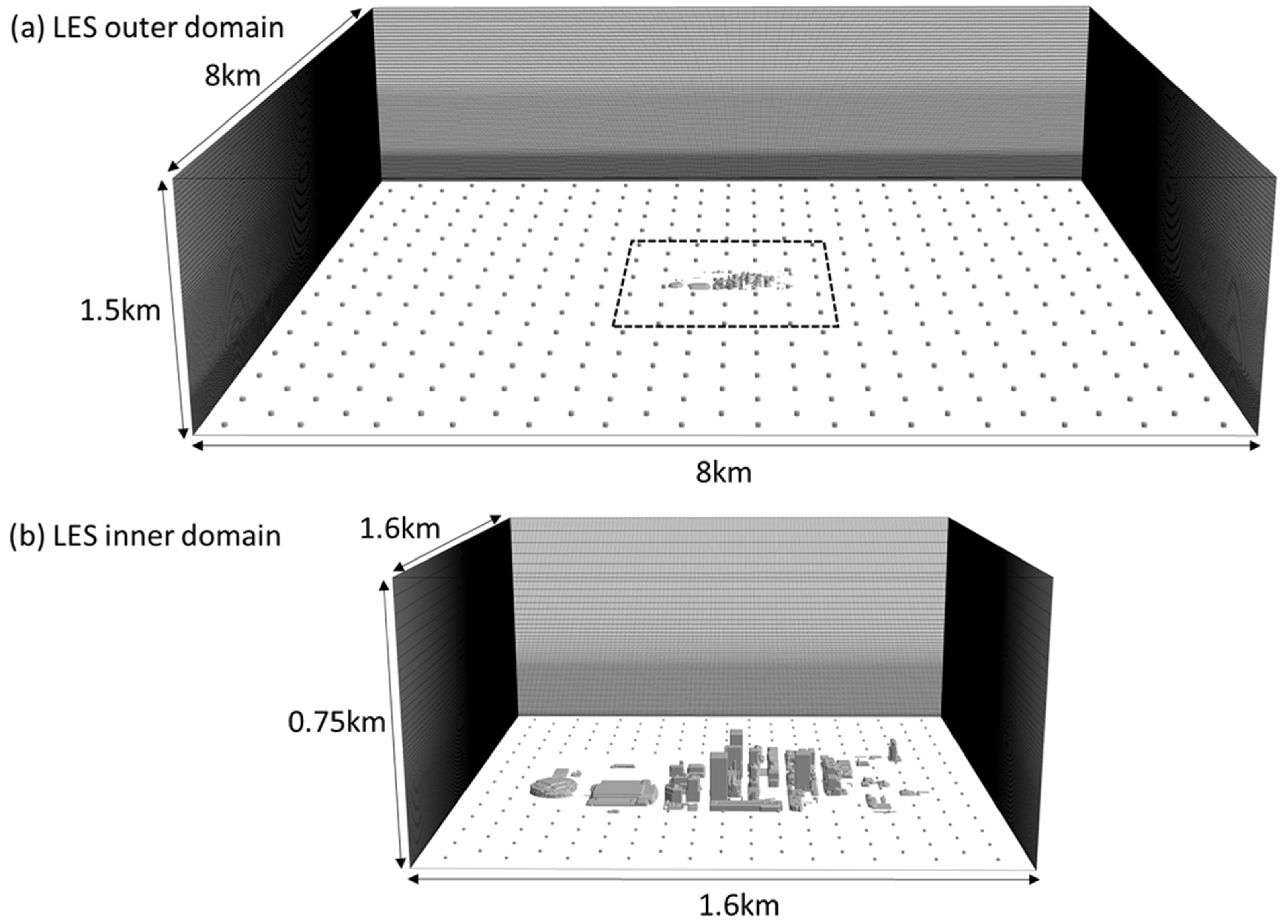
Buildings and structures in the central district of Oklahoma City were explicitly represented by the use of a digital surface model dataset. The turbulent effects are represented by the immersed boundary method [21]. The model is configured using two nested domains with one-way as shown in Figure 3: one is an outer domain for generating atmospheric boundary layer flow and the other is an inner domain for detailed simulations of plume dispersion in the central business district. The outer and inner domains cover areas of 8 km by 8 km by 2.0 km with the grid spacing of 20 m by 20 m by 2–20 m stretched and 1.6 km by 1.6 km by 0.75 km with the grid spacing of 4 m by 4 m by 2–20 m stretched in the streamwise, spanwise and vertical directions.
According to the guidelines for CFD simulations of wind environment in urban areas [22,23], the minimum grid resolution should be 10 grid points to accurately reproduce separating flows around buildings. Individual urban buildings in the LES inner domain are basically resolved by 10 grid points, which are expected to capture the basic patterns of turbulent flows.

3. Coupling with the MMS Model and OBS

The target events are the three 30-min continuous plume release from the Botanical Garden at 0900, 1100, and 1300 Central Daylight Time (CDT) on 16 July in IOP6 for cases1, 2, and 3, respectively. In this study, we compared the concentration data measured by fast-response tracer analyzers with a time response of approximately 1-Hz by Lawrence Livermore National Laboratory.
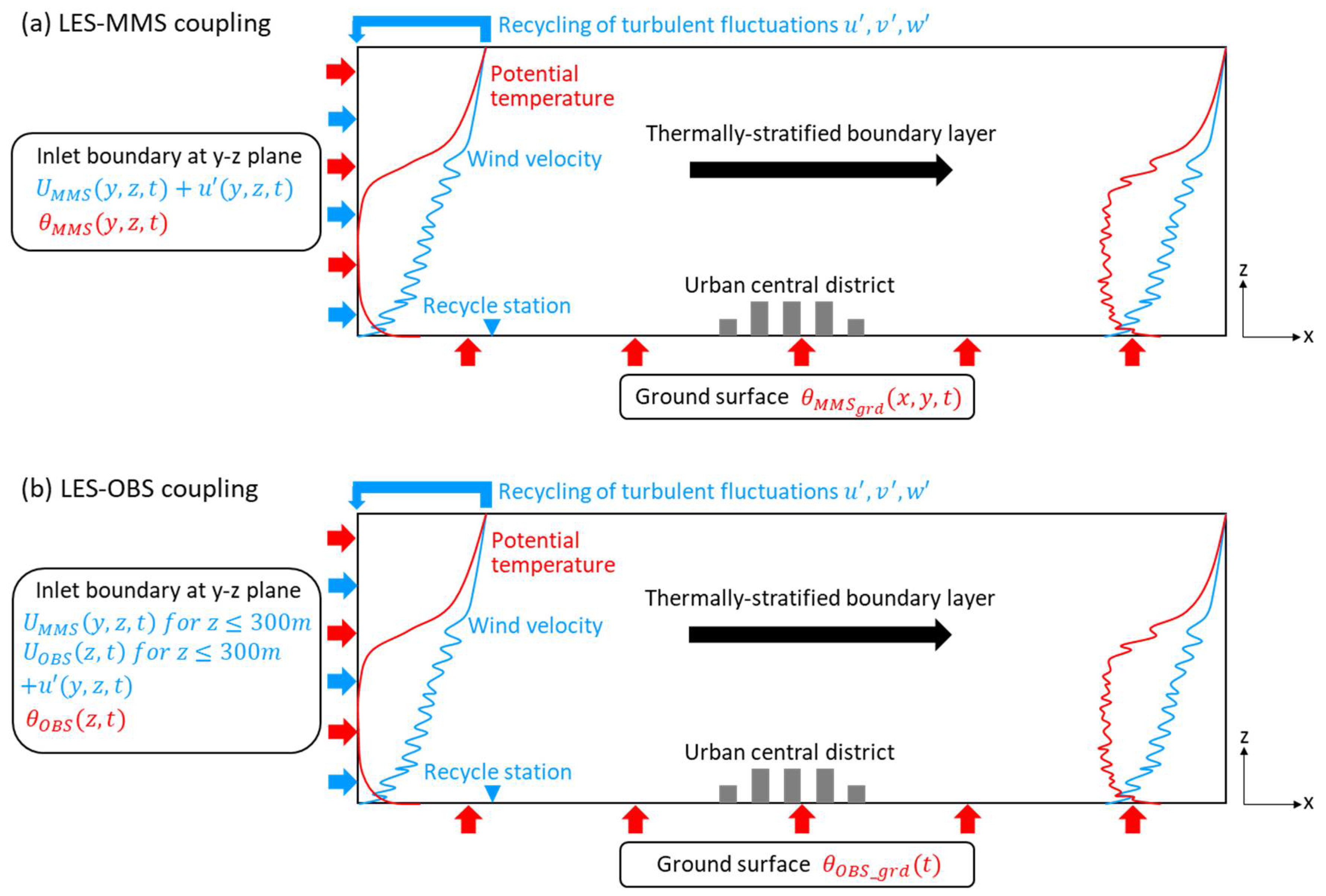
Figure 4 shows schematic of the LES–MMS and LES–OBS coupling cases. For the LES–MMS coupling case, the MMS model data of wind velocities ( U M M S ) and potential temperature ( θ O B S ) of the innermost domain shown in Figure 2 were used as the input conditions of the LES outer domain. First, the atmospheric conditions of IOP6 were reproduced by the MMS model from 1900 CDT 14 July to 1900 CDT 16 July 2003. The first and second inner domains were initialized at 1900 CDT 15 July and at 0700 CDT 16 July, respectively. Then, the boundaries of the inflow and ground surface were determined by the MMS outputs (with 1-min interval and 500-m resolution) linearly interpolated on the grids of the LES outer domain with 1-min interval. On the other hand, for the LES–OBS coupling case, the meteorological observation data obtained at a single stationary point of the OBS1 with 15-min interval from 0700 CDT to 1400 CDT were used as the input conditions of the LES outer domain. Since the dominant mean wind directions were nearly south and the OBS1 was located over the homogeneous ground surface at the upstream position of the urban central district for the target period as shown in Figure 1, the vertical profile of the OBS data obtained at a single stationary point was given at the inflow boundaries under the assumption of horizontal homogeneity. Due to the limitation of the observation range, the upper winds above 300-m height were given by the MMS model data under the condition that the OBS data gradually match with them for the vertical direction. The 15-min averaged OBS data were linearly interpolated on the temporal and spatial resolutions of the LES outer domain and were given as inputs. Furthermore, the input conditions of the LES inner domain were determined by the outputs of the LES outer domain linearly interpolated on the grids of the inner domain with 3-s interval in both coupling cases.
Inflow and outflow boundaries of the LES outer domain are automatically determined in accordance with mean wind direction in the meteorological field. For example, when the mean wind direction lies in the range from 0° to 90°, the vertical planes on the north and east sides are set to inflow boundaries, and those on the south and west sides are set to outflow boundaries. The details were described in Nakayama and Takemi [24]. Each component of the turbulent fluctuations is generated by the recycling method [25]. The following are the formulations at the inflow boundary of the yz vertical plane.
u ( y , z , t ) i n l t = ϕ ( z ) ( u r e c y ( y , z , t ) [ u ( z , t ) ] ) ,
v ( y , z , t ) i n l t = ϕ ( z ) ( v r e c y ( y , z , t ) [ v ( z , t ) ] ) ,
w ( y , z , t ) i n l t = ϕ ( z ) ( w r e c y ( y , z , t ) [ w ( z , t ) ] ) ,
where u ,   v ,   w , and ϕ ( z ) are each components of the turbulent fluctuations and a damping function to control the unwanted development of turbulent fluctuations in the upper part of the simulated boundary layer, respectively. The suffixes of inlt and recy indicate the inlet boundary and the recycle station, respectively. [ u ] , [ v ] , and [ w ] are horizontally averaged winds over the driver region ranging from the inlet boundary to the recycle station, respectively. At the bottom surface, the Monin–Obukhov similarity theory [26] is applied. At the upper boundary, a free-slip condition for the horizontal velocity components and a zero-speed condition for the vertical velocity component are imposed. At the outlet boundary, a free-slip condition is applied for each component of wind velocity.
Table 1 shows input conditions of the two different coupling cases. Here, subscripts i ,   j , and k stand for coordinates (horizontal directions; x ,   y and vertical direction; z ). u ,   u * , and θ are the LES calculated data of the instantaneous wind velocity, the friction velocity, and the potential temperature, respectively. τ i 3 ,   q 3 , ψ m , ψ h , z 0 ,   z 0 T , κ , and t are the local instantaneous local wall stress, the surface heat flux, the stability corrections for momentum and heat, roughness length for momentum and heat, the von Karman constant, and the time, respectively. The suffixes of w s and g r d are the wind speed and ground, respectively. ψ m and ψ h are estimated by the formulation of Businger et al. [27]. z 0 T is estimated by the formulation of Moriwaki and Kanda [28].
The simulation periods of the LES outer and inner domains are from 0700 to 0940 and from 0800 to 0940 for case1, from 0900 to 1140 and from 1000 to 1140 for case2, and from 1100 to 1340 and from 1200 to 1340 for case3, respectively. The calculation time step intervals are 0.2- and 0.02-s in the LES outer and inner domains, respectively.

4. Results

4.1. Flow Field

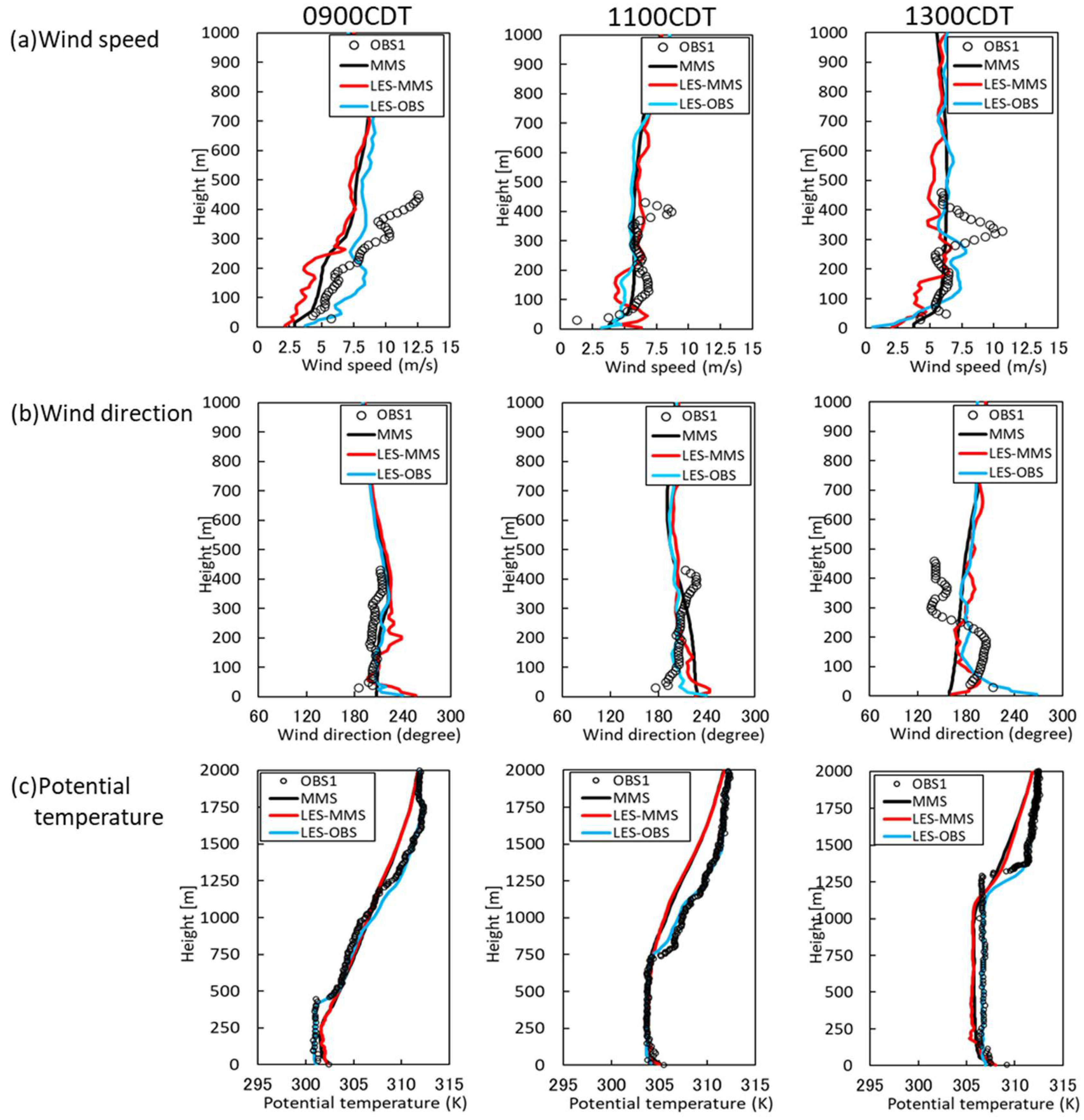
Figure 5 shows vertical profiles of wind speed, wind direction, and potential temperature of the OBS, MMS, LES–MMS, and LES–OBS cases at each plume release time at the OBS1 position. The wind speed of the OBS increased with height at 0900 CDT. With the development of daytime convective boundary layer (CBL), the OBS wind speed gradually became nearly homogeneous up to 300-m height due to the turbulent mixing motions. According to Wyszogrodzki et al. [11], the low-level jet was observed during the early morning in IOP6. The OBS data of the sharp peak in the range of 300–400 m height at 1100 and 1300 CDT were due to the residual low-level jet. As the MMS model did not capture the rapid change of the wind speed, nor was it simulated by the LES–MMS case, the LES–OBS case did not reproduce the low-level jet either, since the upper winds above 300-m height were given by the MMS model. Both cases showed nearly constant vertical profiles of the wind direction at 0900 and 1100 CDT although they did not reproduce the rapid change of the OBS wind directions across 200-m height at 1300 CDT. The potential temperature profiles of the LES–MMS case were similar to the OBS data and those of the LES–OBS were consistent with the OBS at each time point.
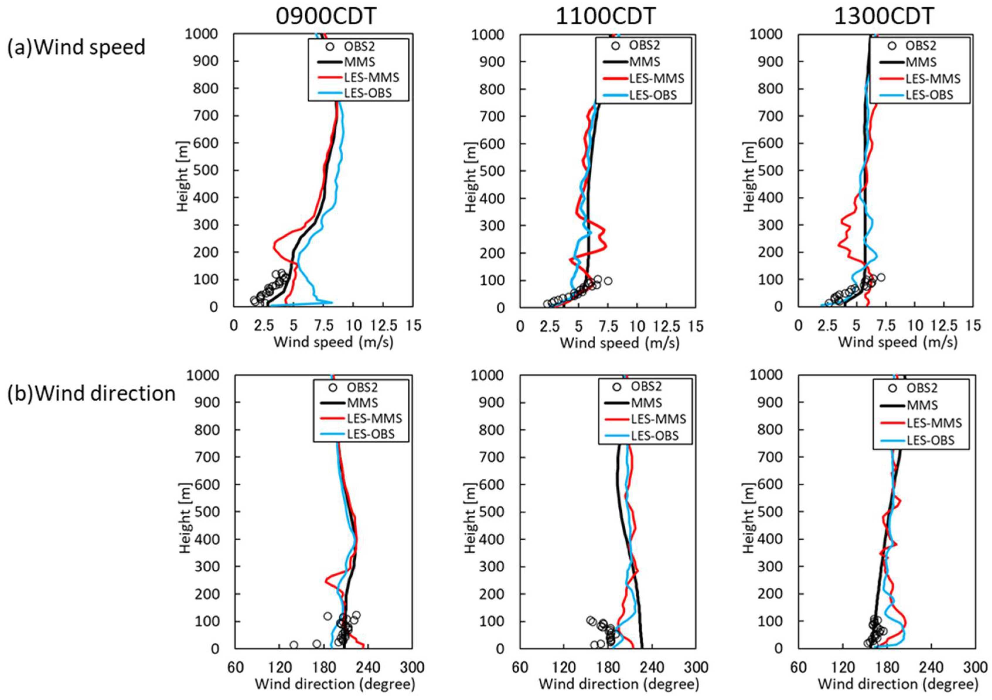
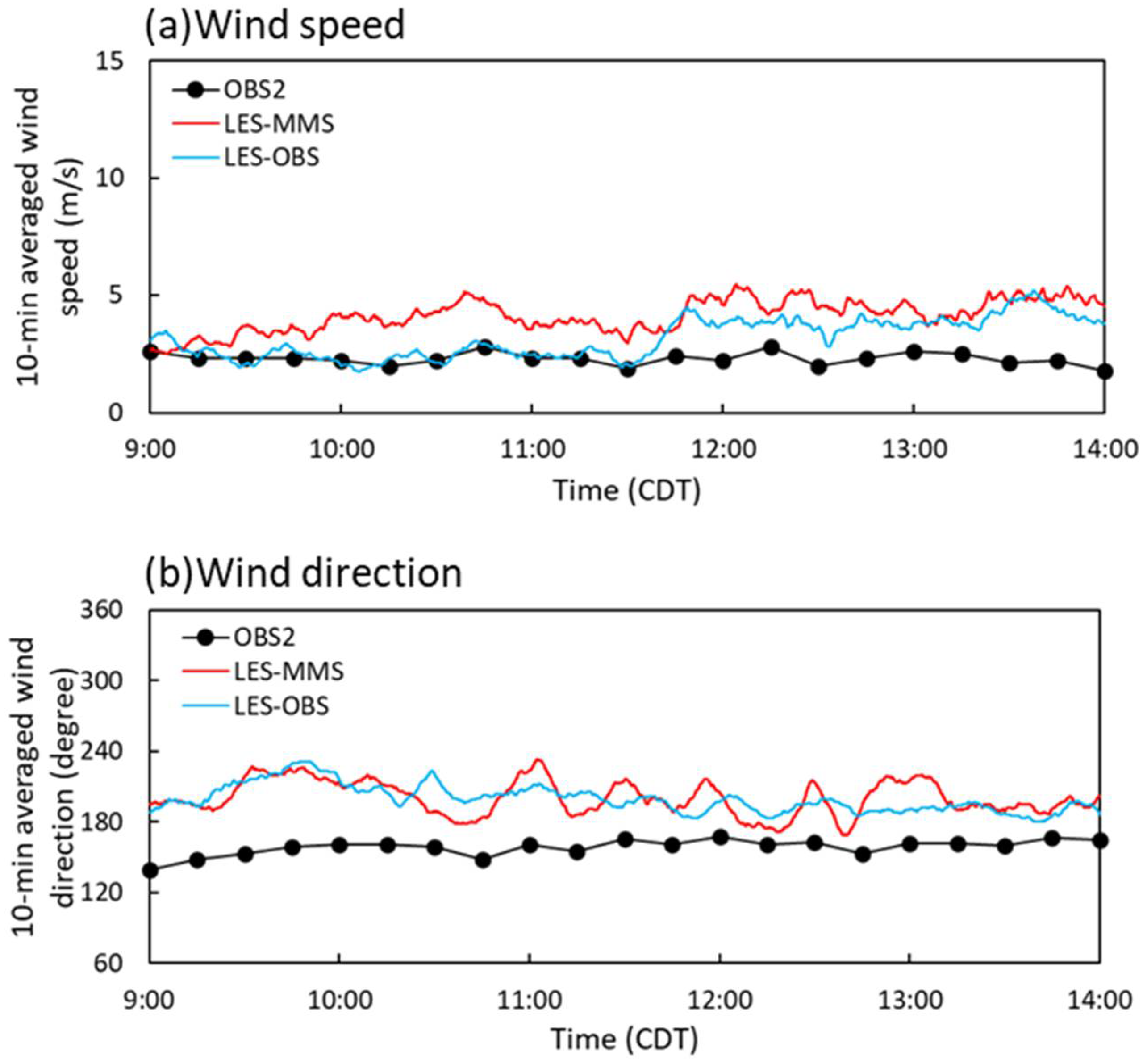
Figure 6 shows the vertical profiles of the wind speed and wind direction at the plume release point. The OBS wind speed rapidly decreases near the ground surface. The OBS wind direction also rapidly varies from the ground surface to 30-m height, especially at 0900 and 1100 CDT. According to the study on turbulent boundary layer flows over urbanlike roughness by Cheng and Castro [8], the flow patterns are directly determined by building arrangements and show a strong three-dimensionality caused by impinging, separated, and recirculating flows in the building canopy layer, while the dynamical influence of the surface decreases with height and the flows eventually readjust to the meteorological conditions. It seems that these rapid changes are due to the influence of various obstacles such as buildings and trees in the Botanical Garden. As these were not explicitly resolved in the MMS models, the LES–MMS case did not reproduce the local variations and rapid decrease in the wind speed and wind direction near the ground surface. The LES–OBS case did not capture such a tendency either. Figure 7 shows the time series data of the wind speed and wind direction of the OBS and the 10-min averaged LES data. These data of both cases are different from the OBS data, although the LES–OBS case was consistent with the OBS data of the wind speed in the morning.
It is found from these results that there are quantitatively differences in the vertical profiles and time series of the wind velocities between the OBS and both LES coupling cases. However, the tendencies of the development of CBL were simulated well by both LES coupling cases. It is also considered from these results that the OBS data obtained at a single stationary point used for the LES–OBS case are reasonable to prescribe the input condition under the assumption of horizontal homogeneity.
There have been many studies on incorporating aerodynamic effects of roughness elements on urban boundary layer flows into MMS models. For example, Wyszogrodzki et al. [11] compared performance of a single-layer urban canopy model (SUCM) and a multilayer urban canopy model (MUCM) used in WRF model. They concluded that WRF–MUCM reproduces the observed mean near-surface and boundary-layer winds and temperature fields during daytime conditions, and provides statistics during the nighttime more accurately than WRF–SUCM. In order to represent urban aerodynamic effects of urban surfaces more accurately by MMS model, such urban canopy models should be used.

4.2. Concentration Field

Figure 8 shows horizontal distributions of the 30-min averaged concentrations near the ground surface after each plume release time for LES–MMS and LES–OBS cases. The horizontal spread of the plume becomes larger with the development of the daytime CBL, and the general distribution patterns were similar between both LES coupling cases. The high-concentration regions in the LES–OBS case were formed mainly around the plume release point and the mean concentrations rapidly decreased with downwind distance, while those in the LES–MMS case were formed along the main street parallel to the mean wind direction at 1300CDT.
Nelson et al. [13] conducted building-resolving detailed simulations of plume dispersion using WRF model data and various meteorological observations, and evaluated them against the Joint Urban 2003 tracer gas measurements. They mentioned that local intermediate-scale variabilities (i.e., between mesoscale and microscale) reproduced by using only an OBS single stationary point as input were represented as if they were sudden changes in the mesoscale wind field, which significantly overpredicted the lateral spread of the plume. There is a possibility that the larger horizontal spread of the plume for the LES–OBS case is due to the use of a single measurement location.
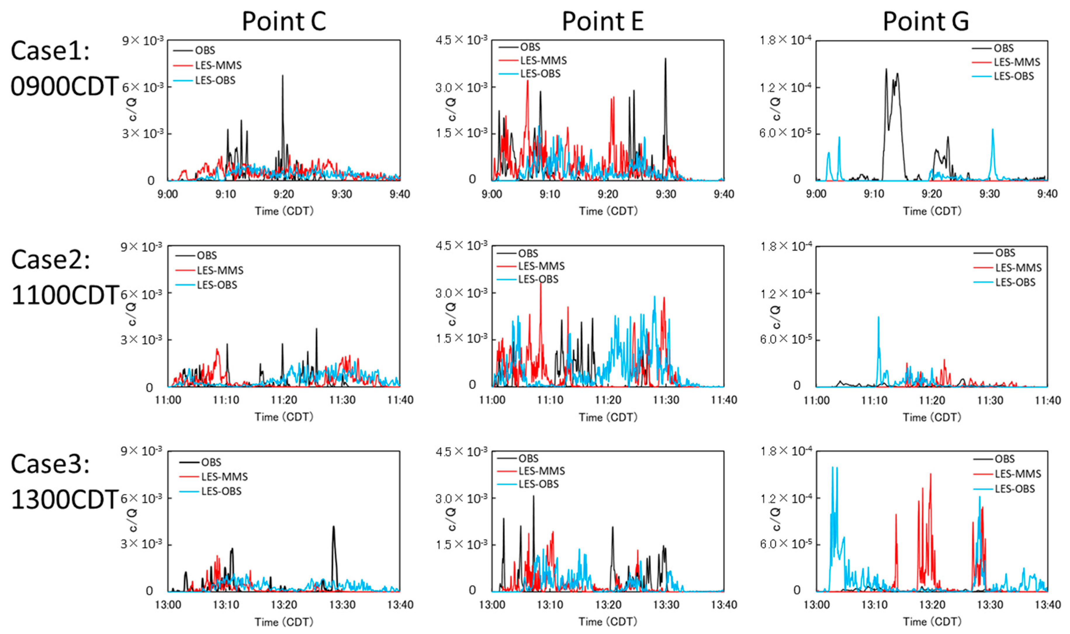
Figure 9 compares time series of concentration fluctuations obtained by the LES–MMS and LES–OBS cases with the field experimental data at the positions of C, E, and G for cases 1, 2, and 3. At point C, instantaneous high concentrations of the field experiments intermittently occur for each case. Those obtained by both coupling cases were less intermittent and were smoother than the experimental values. Thus, the concentration fluctuating patterns were considerably different from the experimental data. According to the LES sensitivity analysis of grid resolution for a point source corresponding to 1.0 and 10 times the real diameter on the plume intermittency by Michioka et al. [29], it was shown that the intermittency of the concentrations was overestimated by the excess subgrid turbulent mixing for a case of a coarse grid. The hose diameter used for continuous gas release in the JU2003 field experiments was approximately 1.6-cm [30], which was far smaller than the grid resolution of 4 m by 4 m set up in this calculation condition. This overestimation of the intermittency is clearly due to the excess action of the subgrid turbulent mixing by a coarse grid resolution. At point E, instantaneous high concentrations frequently occurred in the field experiments for each case. These tendencies were simulated well by both coupling cases. At point G, the concentrations fluctuated with a large time scale and showed high peaks in the experiments, especially for case 1. Both coupling cases showed sharper peak concentrations than the experimental ones. The fluctuating concentration patterns were considerably different from the experimental data.
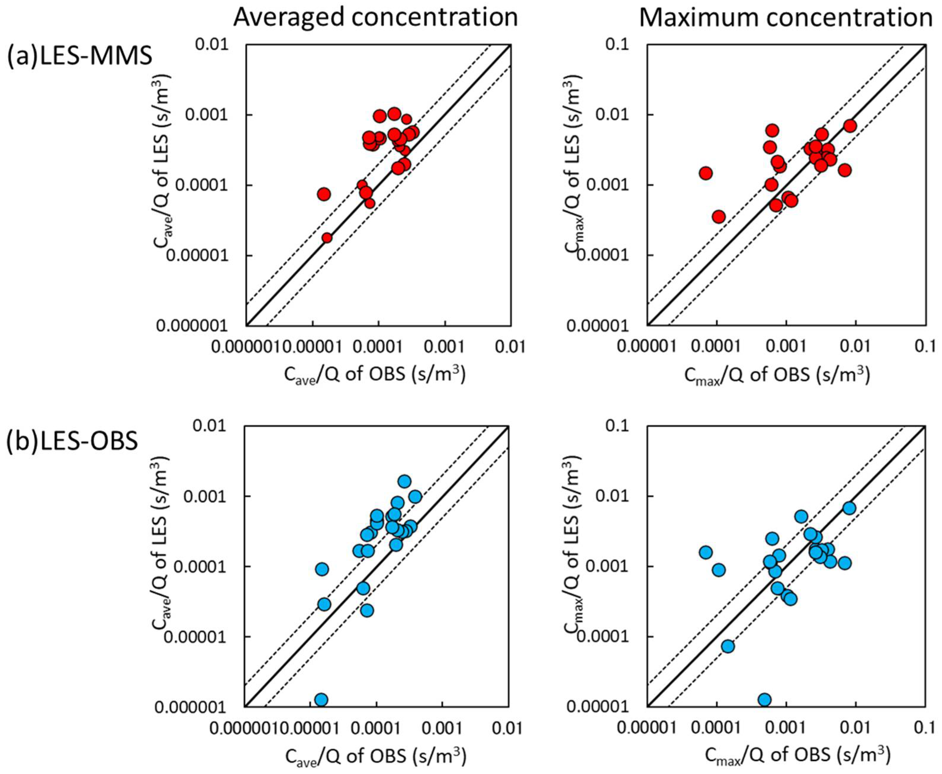
Figure 10 shows a scatter plot of the 30-min averaged and maximum concentrations during the plume release duration time. Here, FAC2, whose value is within 0.5–2.0, is the ratio of the LES data to the OBS data. From this definition, the best results have a value of 1.0. Statistical performance measures for quantitatively evaluating the predictions of a model with field measurements usually include fractional bias (FB), geometric mean bias (MG), normalized mean square error (NMSE), geometric variance (VG), and the fraction of predictions within a factor of 2 of field measurements (FAC2). According to the model performance evaluation study by Chang and Hanna [31], the FAC2 is the most robust performance measure, because it is not overly influenced by either low or high outliers. The mean concentrations of both LES cases were overestimated in the high concentrations. In addition, those of the LES–OBS were comparatively scattered and were somewhat underestimated in the low concentrations. The maximum concentrations of both LES cases were consistent with the OBS data especially in the high concentrations. However, those of the LES–OBS case were comparatively scattered in the low concentrations. Burman et al. [14] conducted LESs of turbulent flows in Oklahoma City and investigated the accuracy of three typical subgrid models in comparison to the field experimental data. They mentioned that in the urban central district, simulated turbulence is mainly determined by buildings and their configurations and is only weakly affected by LES subgrid model type, while outside and upwind of the central district the turbulence given at the inflow boundaries is very important. It seems that the deviations between measured and simulated concentration data within the built-up areas are caused mainly by geometrical simplifications.
The FAC2 of the mean and maximum concentrations were 0.42 and 0.63 for LES–MMS, and 0.30 and 0.58 for LES–OBS, respectively. Various methodologies have been investigated to evaluate the performance of local-scale atmospheric dispersion models [32,33,34,35]. For example, Hanna and Chang [34] suggested that a good model should have FAC2 ≥ 30% for urban areas based on a large number of model evaluation exercises by the field experimental data of mean concentrations. FAC2 of the mean concentrations by the LES–OBS case was comparable to the recommended value, whereas that of the LES–MMS case exceeded it. The peak concentrations obtained by both LES cases were distributed around the perfect line in the high concentrations. As there is no universal definition of acceptable criteria for peak concentrations at present, it is difficult to fully evaluate the model performance for them. However, it can be expected that the peak concentrations were reasonably captured depending on different downwind positions.
It is found from these results that the LES–MMS coupling case show good performance. The LES–OBS one also shows reasonable performance. This indicates that it is effective to prescribe the input conditions using the OBS data obtained even at a single stationary point over the homogeneous ground surface with the assumption of horizontal homogeneity.

5. Conclusions

We conducted LESs of plume dispersion in the urban central district under realistic meteorological conditions by coupling with the MMS model and OBS obtained at a single stationary point, and evaluated the two different cases in comparison with the JU2003 field experiments conducted in the central district of Oklahoma City.
For the LES–MMS coupling case, the MMS model data of wind velocities and potential temperature were used as the input conditions of the LES domain. For the LES–OBS coupling case, the OBS data obtained at a single stationary point were used as the input conditions of the LES domain under the assumption of horizontal homogeneity. Although there were quantitative differences in the vertical profiles and time series of the wind velocities between the OBS and both LES coupling cases, the tendencies of the development of CBL were simulated well. This indicates that the OBS data used for the LES–OBS case was reasonable for prescribing the input condition under the assumption of horizontal homogeneity.
The general distribution patterns of the mean concentrations were similar between both LES coupling cases, although the high-concentration regions were a little different in the daytime CBL development. The fluctuating concentration patterns were considerably different from the field experimental data at several measuring points. This is due to coarse grid resolution for a plume release point. Focusing on a scatter plot of the 30-min averaged and maximum concentrations during the plume release duration time, it was shown that the mean concentrations obtained by both LESs were overestimated in the high-concentration regions. Those of the LES–OBS case were comparatively scattered and were a little underestimated, especially in the low concentrations. The maximum concentrations of both LESs were consistent with the experimental data, especially in the high concentrations. The LES–MMS case showed better performance than the LES–OBS one. However, FAC2 of the latter case was comparable to the acceptance criteria on the model prediction within a factor of two of the field experimental data and showed reasonable performance. This indicates that it is promising to prescribe the input conditions using the OBS data obtained at a single stationary point over the homogeneous ground surface under the assumption of horizontal homogeneity.
In order to further improve the simulation accuracy, the following three points should be considered.
  • Appropriately represent aerodynamic effects of urban surfaces with the MMS model;
  • Utilize multiple spatially varying wind field observations;
  • Incorporate data assimilation techniques into the LES model.
Regarding the first point, one conventional approach to parameterize the effects of buildings and structures is to introduce an urban canopy model. Several researchers [35,36,37] recommended the use of multilayer urban canopy models for appropriately representing urban effects on boundary layer structure. On the second point, Nelson et al. [13] mentioned that using the spatially varying flow fields generated from multiple observation profiles generally provided the best performance from model evaluation against the Joint Urban 2003 tracer gas measurements. Multiple spatially varying meteorological observations are favorable in terms of avoiding unrealistically reproduced temporal and spatial variability by using only a single measurement location as an input. The final point is that it is effective to use a data assimilation technique which is capable of reproducing more realistic simulated states by incorporating observational data into simulation models. In future work, we will apply the data assimilation method using a vibration equation [38] to LESs of plume dispersion in complex urban environments while both nudging the flow fields toward a target mean state and retaining the fluctuating nature of turbulent flows.

Author Contributions

Conceptualization, methodology, writing—original draft preparation, H.N.; writing—review and editing, T.T. and T.Y. All authors have read and agreed to the published version of the manuscript.

Funding

This work was supported by JSPS KAKENHI grant 18H01680 and 21H01591.

Institutional Review Board Statement

Not applicable.

Informed Consent Statement

Not applicable.

Conflicts of Interest

The authors declare no conflict of interest.

References

  1. Inoue, T. CBRN Terrorism & Defense. J. Jpn. Soc. Saf. Eng. 2016, 55, 398–405. (In Japanese) [Google Scholar]
  2. Report of the United Nations Scientific Committee on the Effects of Atomic Radiation to the General Assembly, 2013 Report Vol. I. Sources, Effects and Risks of Ionizing Radiation; United Nations Scientific Committee on the Effects of Atomic Radiation: New York, NY, USA, 2013.
  3. World Health Organization. WHO Air Quality Guidelines for Particulate Matter, Ozone, Nitrogen Dioxide and Sulfur Dioxide: Global Update 2005: Summary of Risk Assessment; WHO: Geneva, Switzerland, 2006. [Google Scholar]
  4. World Health Organization. The invisible killer—Health effects of air pollution. In Proceedings of the First WHO Global Conference on Air Pollution and Health, Geneva, Switzerland, 30 October–1 November 2018; WHO: Geneva, Switzerland, 2018. [Google Scholar]
  5. Hanna, S.R. The exponential probability density function and concentration fluctuations in smoke plumes. Bound. Layer Meteorol. 1984, 29, 361–375. [Google Scholar] [CrossRef]
  6. Efthimiou, G.C.; Bartzis, J.G.; Koutsourakis, N. Modelling concentration fluctuations and individual exposure in complex urban environments. J. Wind Eng. Ind. Aerodyn. 2011, 99, 349–356. [Google Scholar] [CrossRef]
  7. Efthimiou, G.C.; Bartzis, J.G. Atmospheric dispersion and individual exposure of hazardous materials. J. Hazard. Mater. 2011, 188, 375–383. [Google Scholar] [CrossRef]
  8. Cheng, H.; Castro, I.P. Near wall flow over urban-like roughness. Bound. Layer Meteorol. 2002, 104, 229–259. [Google Scholar] [CrossRef]
  9. Warner, S.; Platt, N.; Jeffry, T.; Heagy, J.F. Comparisons of Transport and Dispersion Model Predictions of the URBAN 2000 Field Experiment. J. Appl. Meteorol. 2004, 43, 829–846. [Google Scholar] [CrossRef] [Green Version]
  10. Tewari, M.; Kusaka, H.; Chen, F.; Coirier, W.J.; Kim, S.; Wyszogrodzki, A.; Warner, T. Impact of coupling a microscale computational fluid dynamics model with a mesoscale model on urban scale contaminant transport and dispersion. Atmos. Res. 2010, 96, 656–664. [Google Scholar] [CrossRef]
  11. Wyszogrodzki, A.; Miao, S.; Chen, F. Evaluation of the coupling between mesoscale-WRF and LES-EULAG models for simulating fine-scale urban dispersion. Atmos. Res. 2012, 118, 324–345. [Google Scholar] [CrossRef]
  12. Nelson, M.A.; Brown, M.J.; Halverson, S.A.; Bieringer, P.; Annunzio, A.; Bieberbach, G.; Meech, S. A case study of the weather research and forecasting model applied to the joint urban 2003 tracer field experiment. Part 1: Wind and turbulence. Bound. Layer Meteorol. 2016, 158, 285–309. [Google Scholar] [CrossRef]
  13. Nelson, M.A.; Brown, M.J.; Halverson, S.A.; Bieringer, P.; Annunzio, A.; Bieberbach, G.; Meech, S. A Case Study of the Weather Research and Forecasting Model Applied to the Joint Urban 2003 Tracer Field Experiment. Part 2: Gas Tracer Dispersion. Bound. Layer Meteorol. 2016, 161, 461–490. [Google Scholar] [CrossRef]
  14. Burman, J.; Jonsson, L.; Rutgersson, A. On possibilities to estimate local concentration variations with CFD-LES in real urban environments. Environ. Fluid Mech. 2019, 19, 719–750. [Google Scholar] [CrossRef] [Green Version]
  15. Li, H.; Cui, G.; Zhang, Z. A New Scheme for the Simulation of Microscale Flow and Dispersion in Urban Areas by Coupling Large-Eddy Simulation with Mesoscale Models. Bound. Layer Meteorol. 2018, 167, 145–170. [Google Scholar] [CrossRef]
  16. Allwine, K.J.; Flaherty, J.E. Joint Urban 2003 Study Overview and Instrument Locations; PNNL-15967; Pacific Northwest National Laboratory: Richland, WA, USA, 2003. [Google Scholar]
  17. Nakayama, H.; Takemi, T.; Nagai, H. Development of local-scale high-resolution atmospheric dispersion model using large-eddy simulation part5: Detailed simulation of turbulent flows and plume dispersion in an actual urban area under real meteorological conditions. J. Nucl. Sci. Technol. 2016, 53, 887–908. [Google Scholar] [CrossRef]
  18. Skamarock, W.C.; Klemp, J.B.; Dudhia, J.; Gill, D.O.; Barker, D.M.; Duda, M.G.; Huang, X.; Wang, W.; Powers, J.G. A Description of the Advanced Research WRF Version 3; NCAR Tech. Note, NCAR/TN-475+STR; National Center for Atmospheric Research: Boulder, CO, USA, 2008; p. 1. [Google Scholar]
  19. Janjic, Z.I. Nonsingular Implementation of the Mellor-Yamada Level 2.5 Scheme in the NCEP Meso Model; NCEP Office Note; National Centers for Environmental Prediction: Camp Springs, MD, USA, 2002; Volume 437, p. 61. [Google Scholar]
  20. Meneveau, C.; Lund, T.; Cabot, W. A Lagrangian dynamic sub-grid-scale model of turbulence. J. Fluid Mech. 1996, 319, 353–385. [Google Scholar] [CrossRef] [Green Version]
  21. Goldstein, D.; Handler, R.; Sirovich, L. Modeling a no-slip flow boundary with an external force field. J. Comput. Phys. 1993, 105, 354–366. [Google Scholar] [CrossRef] [Green Version]
  22. Franke, J.; Hellsten, A.; Schlunzen, H.; Carissimo, B. Best Practice Guideline for the CFD Simulation of Flows in the Urban Environment, COST Action 732, Quality Assurance and Improvement of Microscale Meteorological Models; Meteorological Inst.: Brussels, Belgium, 2007; ISBN 3-00-018312-4. [Google Scholar]
  23. Tominaga, Y.; Mochida, A.; Yoshie, R.; Kataoka, H.; Nozu, T.; Yoshikawa, M.; Shirasawa, T. AIJ guidelines for practical applications of CFD to pedestrian wind environment around buildings. J. Wind Eng. Ind. Aerodyn. 2008, 96, 1749–1761. [Google Scholar] [CrossRef]
  24. Nakayama, H.; Takemi, T. Large-eddy simulation studies for predicting plume concentrations around nuclear facilities using an overlapping technique. Int. J. Environ. Pollut. 2018, 64, 125–144. [Google Scholar] [CrossRef]
  25. Kataoka, H.; Mizuno, M. Numerical flow computation around aeroelastic 3D square cylinder using inflow turbulence. Wind Struct. 2002, 5, 379–392. [Google Scholar] [CrossRef]
  26. Monin, A.; Obukhov, M. Basic laws of turbulent mixing in the ground layer of the atmosphere. Tr. Akad. Nauk SSSR Geophiz. Inst. 1954, 24, 163–187. [Google Scholar]
  27. Businger, J.A.; Wyngaard, J.C.; Izumi, Y.; Bradley, E.F. Flux-profile relationships in the atmospheric surface layer. J. Atmos. Sci. 1971, 28, 181–189. [Google Scholar] [CrossRef]
  28. Moriwaki, R.; Kanda, M. Flux-gradient profiles for momentum and heat over an urban surface. Theor. Appl. Climatol. 2006, 127–135. [Google Scholar] [CrossRef]
  29. Michioka, T.; Sato, A.; Sada, K. Large-eddy simulation for the tracer gas concentration fluctuation in atmospheric boundary layer. Trans. Jpn. Soc. Mech. Eng. 2003, B69, 868–875. (In Japanese) [Google Scholar] [CrossRef]
  30. Warner, S.; Urban, J.T.; Heagy, J.F. Comparisons of T&D model predictions of the Joint Urban 2003 field experiment. J. Appl. Meteorol. Climatol. 2008, 47, 1910–1928. [Google Scholar]
  31. Chang, J.C.; Hanna, S.R. Air quality model performance evaluation. Meteorol. Atmos. Phys. 2004, 87, 167–196. [Google Scholar] [CrossRef]
  32. Hanna, S.R.; Hansen, O.R.; Dharmavaram, S. FLACS CFD air quality model performance evaluation with Kit Fox, MUST, Prairie Grass, and EMU observations. Atmos. Environ. 2004, 38, 4675–4687. [Google Scholar] [CrossRef]
  33. Hanna, S.R.; Chang, J.C. Acceptance criteria for urban dispersion model evaluation. Meteorol. Atmos. Phys. 2012, 116, 133–146. [Google Scholar] [CrossRef]
  34. Herring, S.; Huq, P. A review of methodology for evaluating the performance of atmospheric transport and dispersion models and suggested protocol for providing more informative results. Fluids 2018, 3, 20. [Google Scholar] [CrossRef] [Green Version]
  35. Martilli, A.; Clappier, A.; Rotach, M.W. An urban surface exchange parameterisation for mesoscale models. Bound. Layer Meteorol. 2002, 104, 261–304. [Google Scholar] [CrossRef]
  36. Kondo, H.; Tokairin, T.; Kikegawa, Y. Calculation of wind in a Tokyo urban area with a mesoscale mode lincluding a multi-layer urban canopy model. J. Wind Eng. Ind. Aerodyn. 2008, 96, 1655–1666. [Google Scholar] [CrossRef]
  37. Salamanca, F.; Martilli, A.; Tewari, M.; Chen, F. A study of the urban boundary layer using different urban parameterizations and high-resolution urban canopy parameters with WRF. J. Appl. Meteorol. Climatol. 2011, 50, 1107–1128. [Google Scholar] [CrossRef]
  38. Nakayama, H.; Takemi, T. Development of a data assimilation method using vibration equation for large-eddy simulations of turbulent boundary layer flows. J. Adv. Model. Earth Syst. 2020, 12. [Google Scholar] [CrossRef]
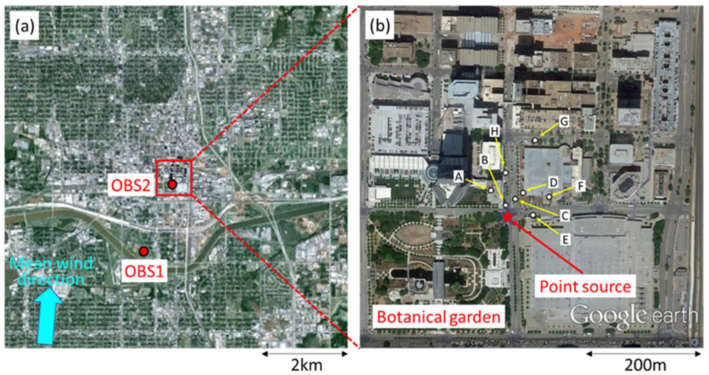
Figure 1. Locations of meteorological stations (a) and concentration measurement in the central business district of Oklahoma City (b). The star mark depicts a point source position which corresponds to the meteorological station OBS2. Time series of concentration fluctuations obtained at points A–H are used for the model evaluation. The photograph is reproduced by GoogleTM earth graphic.
Atmosphere 12 00889 g001
Figure 2. Computational areas of the MMS model. The MMS model is configured with three nested domains covering areas of (a) 2700 km × 2700 km at 4.5 km grid, (b) 600 km × 600 km at 1.5 km grid, and (c) 150 km × 150 km at 500 m grid [17].
Atmosphere 12 00889 g002
Figure 3. LES computational domains and mesh arrangement. The LES model is configured with two nested domains: (a) the outer domain of 8 km × 8 km at 20 m grid for generating atmospheric boundary layer flow and (b) the inner domain of 1.6 km × 1.6 km at 4 m grid for detailed simulations of plume dispersion in the central business district [17]. The dashed line in (a) the outer domain indicates (b) the inner domain.
Atmosphere 12 00889 g003
Figure 4. Schematic of (a) LES–MMS and (b) LES–OBS coupling cases.
Atmosphere 12 00889 g004
Figure 5. Vertical profiles of wind speed (a), wind direction (b), and potential temperature (c) of the OBS, MMS, LES–MMS, and LES–OBS cases at each plume release time at the position of the OBS1.
Atmosphere 12 00889 g005
Figure 6. Vertical profiles of the wind speed (a) and wind direction (b) of the OBS, MMS, LES–MMS, and LES–OBS cases at the plume release point.
Atmosphere 12 00889 g006
Figure 7. Time series of the wind speed (a) and wind direction (b) at 15-m height.
Atmosphere 12 00889 g007
Figure 8. Horizontal distributions of the 30-min averaged concentrations near the ground surface after each plume release time for cases of LES-MMS (a) and LES-OBS (b) cases. The circle mark depicts the plume source point.
Atmosphere 12 00889 g008
Figure 9. Time series of concentrations fluctuations of the OBS, the LES–MMS and LES–OBS cases.
Atmosphere 12 00889 g009
Figure 10. Scatter plot of the 30-min averaged and maximum concentrations in the LES–MMS (a) and LES–OBS (b) cases. The solid and dashed lines indicate the perfect and FAC2 lines, respectively.
Atmosphere 12 00889 g010
Table 1. Input conditions of the LES–MMS and LES–OBS coupling cases.
Input DataLES–MMS Coupling CaseLES–OBS Coupling Case
Wind
velocity
field
Inlet U M M S ( y , z , t ) + u ( y , z , t ) U O B S ( z , t ) + u ( y , z , t )
Ground
surface
τ i 3 = ( u w s _ g r d ( x , y , t ) κ l n ( z / z 0 ) ψ m ) 2 u i _ g r d ( x , y , t ) u w s _ g r d ( x , y , t )
Potential
temperature
field
Inlet θ M M S ( y , z , t ) θ O B S ( z , t )
Ground
surface
q 3 = u * κ ( θ M M S _ g r d ( x , y , t ) θ g r d ( x , y , t ) ) l n ( z / z 0 T ) ψ h q 3 = u * κ ( θ O B S _ g r d ( t ) θ g r d ( x , y , t ) ) l n ( z / z 0 T ) ψ h
Publisher’s Note: MDPI stays neutral with regard to jurisdictional claims in published maps and institutional affiliations.