Abstract
To evaluate the effectiveness of measures to reduce the levels of volatile organic compounds (VOCs), which are important precursors of ground-level ozone formation, the real-time monitoring data of VOCs at the urban Zhaohui supersite (ZH), the Dianshan Lake regional supersite (DSL) and the urban Yixing station (YX) in the Yangtze River Delta region were analyzed from 23 August to 15 September 2016 during the G20 Hangzhou Summit. The average mole ratios of VOCs at the three sites were 6.56, 21.33 and 19.62 ppb, respectively, which were lower than those (13.65, 27.72 and 21.38 ppb) after deregulation. The characteristics of the VOCs varied during the different control periods. Synoptic conditions and airmass transport played an important role in the transport and accumulation of VOCs and other pollutants, which affected the control effects. Using the positive matrix factorization (PMF) method in source apportionment, five factors were identified, namely, vehicle exhaust (19.66–31.47%), plants (5.59–17.07%), industrial emissions (13.14–33.82%), fuel vaporization (12.83–26.34%) and solvent usage (17.84–28.95%) for the ZH and YX sites. Factor 4 was identified as fuel vaporization + incomplete combustion (21.69–25.35%) at the DSL site. The Non-parametric Wind Regression (NWR) method showed that regional transport was the main factor influencing the VOC distribution.
1. Introduction
As the largest developing country in the world, China has suffered from serious air pollution throughout the processes of rapid urbanization and motorization [1]. The occurrence of air pollution caused by high levels of ozone and/or fine secondary aerosol particles in megacities is very severe and complex [2,3,4,5]. As one of the key precursors for secondary organic aerosols (SOA) and ground-level ozone formation, volatile organic compounds (VOCs) play significant roles in our understanding of the formation mechanism of SOA [2,6,7,8,9] and ozone [10,11,12].
Recent studies have mainly focused on the characteristics and sources of VOCs in China’s megacities and city clusters, such as the Beijing–Tianjin–Hebei (BTH) region [13], the Yangtze River Delta (YRD) region [14,15,16], the Pearl River Delta (PRD) region [17,18,19,20] and the megacities of Beijing [21,22,23], Shanghai [24,25] and Nanjing [26]. These studies found that vehicle emissions and solvent usage contributed most to the ambient VOCs in urban areas. Here, the mixing ratio and chemical composition of ambient VOCs in the YRD region was investigated. The biogenic and anthropogenic emissions were estimated. The Non-parametric Wind Regression (NWR) method was used to identify the regional transport.
To improve the air quality when large-scale games and events are held in China, a series of control measures are implemented [27] showed that the photochemical consumption of reactive hydrocarbons (HCs) and the photochemical initial concentrations (PICs) of seven key reactive species were reduced by 39% as a result of the control measures. The emission strength of VOCs was estimated during the 2010 Shanghai World Expo. According to the study, VOCs emission in Shanghai per hour resulted in the VOCs mole ratio increment of (5.98 ± 3.18) × 10−9, during the 2010 EXPO, which was decreased by about 1 × 10⁻⁹ compared to that in the same period of 2009 [28]. These studies mainly focused on the measurements of VOCs in only one city. A few studies [13,29] were conducted to evaluate the joint control of three provinces and one city. The “G20 Blue” program provided the opportunity to investigate changes in air pollutant emissions and ambient air concentrations at different sites. Furthermore, a regional perspective was used here to understand the effectiveness of control measures conducted in the YRD region.
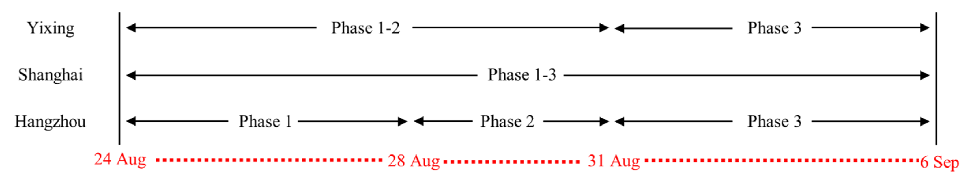
To achieve the “Environmental Quality Guarantee Scheme for Zhejiang Province during the G20 2016 Hangzhou Summit,” the Ministry of Environmental Protection enforced a temporary three-phase emission control scheme in Hangzhou and the surrounding regions within 100 km from Hangzhou [30]. The control regions were divided into three areas: Core area, strictly controlled area and controlled area [31]. Relying on the platform of “G20 Summit guaranteed air quality prediction and forecast system for the YRD region,” real-time monitoring data of VOCs from 12 stations in the YRD region were collected. To discuss the effects of different control measures in different control areas, the urban Zhaohui supersite (ZH) in Hangzhou City, the Dianshan Lake regional supersite (DSL) in Shanghai City and the urban Yixing station (YX) in Yixing City during the 2016 G20 Summit in Hangzhou were chosen, since Hangzhou City was located in the core area, and Shanghai and Yixing City were located in the controlled area. As shown in Figure 1, Table 1 and Table S1 of Supplementary Materials, during the control period (24 August–6 September 2016), different control schemes and different control phases have been implemented in the three cities. After 7 September, all control schemes were stopped, i.e., the deregulation period. According to the positive matrix factorization (PMF) model and NWR techniques, this paper compared the source apportionment and regional transport contribution during the control period and the deregulation period at the three sites. These results could provide potential information for the implementation of emission reduction policies for the establishment of VOC abatement measures in the YRD region.
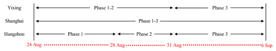
Figure 1.
Time periods corresponding to the different control phases in Hangzhou, Shanghai and Yixing.

Table 1.
Different control periods in Hangzhou.
2. Methods
2.1. Sampling Sites
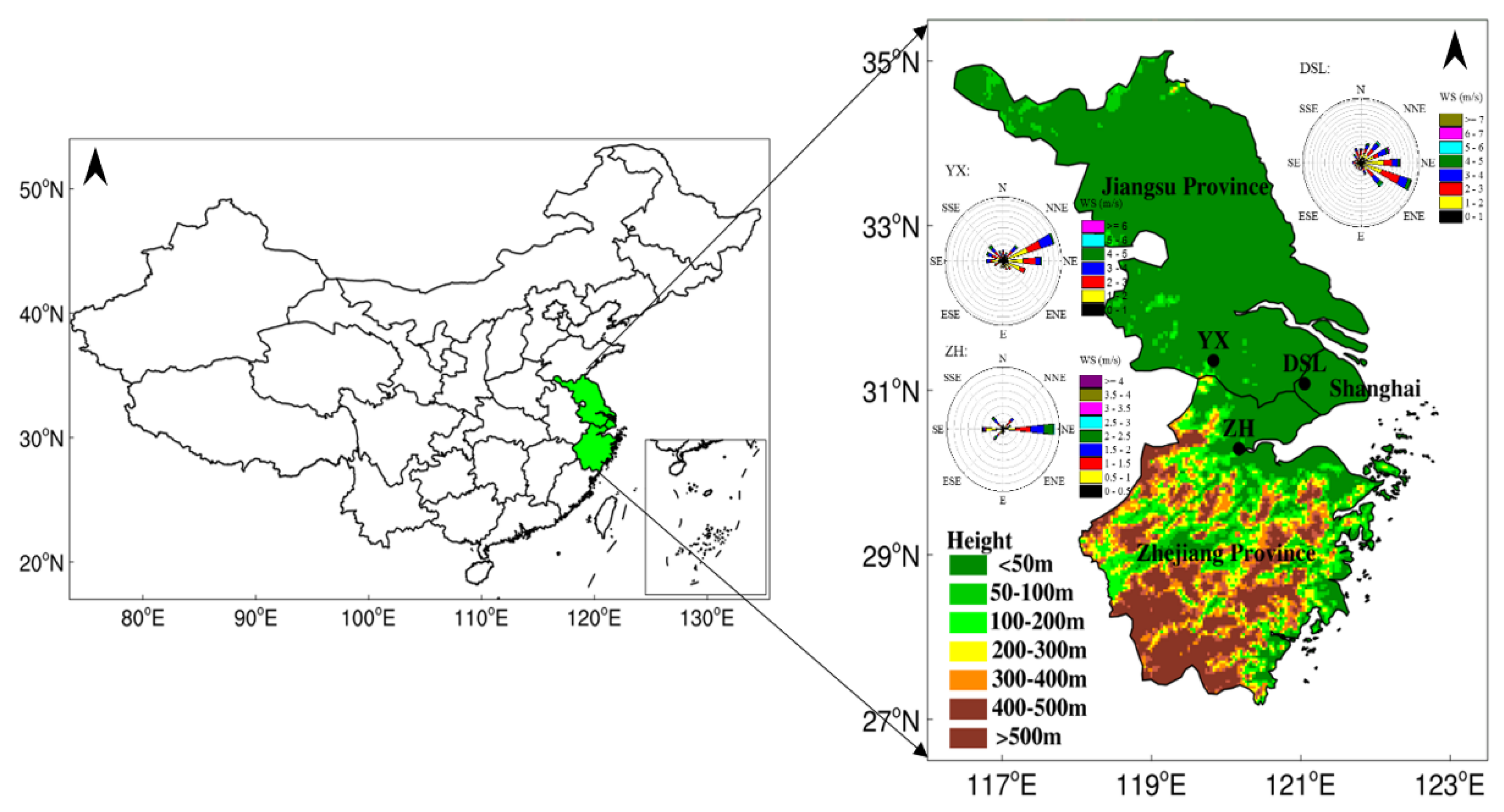
To determine the characteristics of ambient VOCs in the YRD region during the G20 Summit, VOC sampling was conducted at three sites: The urban Zhaohui supersite (ZH), the Dianshan Lake regional supersite (DSL) and the urban Yixing City Environmental Protection Bureau station (YX) (Figure 2). As the venue of the G20 Summit, Hangzhou is located on the southeast coast of China, north of Zhejiang Province, the lower reaches of the Qiantang River and the southern end of the Beijing-Hangzhou Grand Canal. It is a core city in the Hangzhou Bay Greater Bay Area, a central city in the Shanghai-Jiaxing-Hangzhou G60 Science and Technology Innovation Corridor and an important international e-commerce center. As a national central city, Shanghai is located at the estuary of the Yangtze River. It is a leading city in the Yangtze River Economic Belt, located to the northeast of Hangzhou. Yixing, located in the southwestern tip of Jiangsu Province, the center of the Shanghai-Nanjing-Hangzhou triangle and the northwest of Hangzhou, is a national ecological civilization construction model city and county. ZH (30.29° N, 120.17° E) is the central site, located in the city of Hangzhou. The surrounding areas are mainly residential areas, and the main sources of air pollution are traffic and residential. DSL (31.09° N, 120.98° E) is located in Qingpu District, Shanghai City. The site is surrounded by Dianshan Lake and is close to urban arterial roads (~2.5 km southeast of the Shanghai-Chongqing Expressway); moreover, Dianshan Lake is surrounded by villages. YX (31.35° N, 119.82° E) is located in Yixing City, and the surrounding area is mainly distributed by residents, businesses and schools. DSL and YX are located in the northeast and northwest of ZH, respectively. The three sites generally represent the air quality of the G20 in the host and surrounding cities in the YRD region.
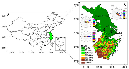
Figure 2.
Location of urban Zhaohui supersite, Dianshan Lake regional supersite and urban Yixing station.
2.2. Observational Instrumentation
The measurement of VOCs at the ZH site was conducted from 23 August to 10 September 2016, while the VOC samples at the DSL and YX sites were collected during the period of 24 August to 15 September 2016. Hydrocarbons (HCs), halocarbon and carbonyls were measured at the DSL and YX sites, but only HCs were measured at the ZH site; of these, the data for acetylene could not be used since the detection rate was lower than 10%. Fifty-seven ambient VOCs, including 30 alkanes, 9 alkenes, 1 alkyne (acetylene) and 17 aromatics, are designated as ozone precursors by the Photochemical Assessment Monitoring Station (PAMS). In this study, 56 VOC (PAMS) species were selected at the three sites since m/p xylene was measured as a single species. The missing values were due to instrument power failure or maintenance and were not included in the data analysis.
The ambient VOCs at the ZH site were collected and analyzed continuously and automatically using an online gas chromatography (GC) system with a temporal resolution of 0.5 h, i.e., a Syntech Spectras GC 955 analysis system (Hangzhou Focused Photonics Inc., Hangzhou, China). Two analyzers, GC 955-611 for high boiling point C6-C12 monitoring and GC 955-811 for low boiling point C2-C5 monitoring, constitute the system. The ambient air sample passes through the Nafion drying tube and then directly enters the analysis system at atmospheric pressure. A cooling preconcentration system, where the VOCs were preconcentrated through carbon molecular sieves (Carbosieve S-III) at 5 °C, was installed in the GC 955-811. Then, thermal desorption was conducted. The C2-C5 VOCs were separated by a two-dimensional chromatographic column with a capillary membrane column and a capillary porous-layer open-tabulator (PLOT) column. C6-C12 were separated on an ATTM-1 column to achieve an optimal separation and to prevent interference from other unrelated compounds. The use of a photoionization detector (PID) and flame ionization detector (FID) ensured high sensitivity and high selectivity.
The VOCs at the DSL site were quantified every 0.5 h by Chromatotec 655 (Shanghai Xiangde Environmental Protection Technology Co., Ltd., Beijing, China). Two different automated GCs equipped with flame ionization detector (GC-FID) systems (Chromatotec GC-866 airmoVOC C2-C6 #58850712 and airmoVOC C6-C12 #283607112) were used to continuously measure the VOCs in ambient air. An in-depth description of the sampling setup, analyzer and technical information (sampling flows, preconcentration, desorption–heating times, types of traps and columns, etc.) can be found in Gros et al. [32].
At the YX site, the VOCs were continuously sampled and measured using TH-300B (Wuhan Tianhong Instrument Co., Ltd., Wuhan, China), an online monitoring system with a temporal resolution of 1 h. The sampling and analysis procedures are described only briefly here since they are described in detail elsewhere [33]. To analyze the VOCs separately, two channels were installed. The system consists of three parts: A cryogenic refrigeration unit, a VOC sampling and preconcentration system and a GC system with a mass spectrometer detector (MSD, Agilent 5975) and FID (Agilent 7890). C2-C5 were separated by a PLOT column and were quantified with a GC-FID. C5-C12 were separated by a DB-624 column and were quantified with an MSD.
At the three sites, 56 PAMS species were calibrated by standard gas for Synspec, the mixture of PAMS and TO15 for Chromatotec and TH-300B (The standard gas concentration of the quality control samples is 2 ppb). The equipment calibrations and verifications through the five-point method were conducted every 2 weeks. The correlation coefficient usually varied from 0.991–0.999 for Synspec, 0.993 to 0.999 for Chromatotec and 0.991 to 0.998 for TH-300B. The detection limit of the instrument is 0.4 µg·m−3 (trans-2-butene) at the ZH site, 0.064 µg·m−3 (benzene) at the DSH site and <3pgC/s (tridecane) at the YX site. The value difference detected by standard samples every day were less than 20%. The relative error of sampling flow rate is 0.6% for the ZH site, <5% for the DSH site and <5% for the YX site. Moreover, the G20 Instrument Assurance Group compared the standard samples at different sites every week to ensure that the data from different instruments were comparable.
2.3. Data Sources
Other datasets including the hourly meteorological parameters (temperature, T; relative humidity, RH; wind speed, WS; and wind direction, WD) were collected from the provincial meteorological observatory, and trace gases (PM2.5, O3 and NO2) were collected from the automatic air quality monitoring station at the three sites. The boundary layer height (BLH) was computed every 3 h each day through NOAA’s READY Archived Meteorology website (http://www.ready.noaa.gov/READYamet.php (accessed on 2 February 2021)).
2.4. Modeling Methodology
2.4.1. Backward Trajectory Analysis
The 24 h backward trajectories with 2 h intervals (starting from 00:00 to 20:00 local time, LT) were run each day at the ZH site by the TrajStat-plug-in of MeteoInfo software, using the Hybrid Single-Particle Lagrangian Integrated Trajectory (HYSPLIT) model [34,35]. The start height was set as 500m above ground level [36]. The FNL global analysis data produced by the National Center for Environmental Prediction’s Global Data Assimilation System (GDAS) wind field reanalysis were introduced into the calculation.
2.4.2. Positive Matrix Factorization (PMF)
The PMF model [37], performed with the EPA PMF 5.0 toolkit, was used to investigate the sources of observed VOCs in the present study. The PMF approach can be explained by the following equations:
X = G × F + E
In Equation (1), let sample X be an i × j matrix. The symbols i and j denote the number of samples and components, respectively. The X matrix can be decomposed by the G and F matrixes, where G = i × p is the emission source contribution matrix and F = p × j is the component spectrum of the pollution source matrix. P denotes the number of pollution sources. The matrix E denotes the difference between X and G × F, i.e., residual matrix. Equations (2) and (3) denote the PMF receptor model method. The basic principle is to calculate the errors of each chemical component in the particulate matter by first using the weight. Then, the main pollution sources and their contribution rates are determined by the least-squares method. Q is a critical parameter for PMF and solved by an iterative minimization algorithm. The Q value is required to be as small as possible. Two versions of Q (Qtrue and Qrobust) are displayed for the model runs. Qtrue is the goodness-of-fit parameter calculated including all points. Qrobust is the goodness-of-fit parameter calculated excluding points not fit by the model, defined as samples for which the uncertainty-scaled residual is greater than 4 [38].
Missing data values were replaced by median concentrations and data values below the method detection limit (MDL) were replaced by MDL/2 [39]. If the concentration is equal to or less than the MDL provided, the uncertainty is calculated using Equation (4). If the concentration is greater than the MDL provided, the calculation follows Equation (5). Error Fraction is the average percent of uncertainty in the whole sampling and analysis process and was set as 0.1 in our study [40].
Not all 56 VOC species were used into the PMF model. The species whose signal-to-noise ratio (S/N) was less than 0.5 were set to bad, and those whose S/N ratios were between 0.5–1.0 were set to weak [38]. Species that include more than 60% of the null value were excluded. Meanwhile, the residual scale of species out of the range of ±3 and correlation between observed and predicted values less than 0.5 were characterized as weak.
In optimizing the Q value, it is also necessary to take into account that the number of sources chosen makes physical sense. In general, the selection range of the number of factors was 3–8 [36]. The Q values are shown in Figure S1. Qexcept is equal to (number of non-weak data values in X)-(number of elements in G and F, taken together) [38]. In theory, if the number of factors was properly estimated, the Qtrue value would be close to the Qexcept value. Instead, the Q value may deviate from the theoretical value [36]. The change between the Q value due to the number of factors at the three sites is shown in Figure S1. At the ZH and DSL sites, the Qtrue/Qexcept value decreased between 3 to 4 factors, indicating that a substantial amount of the variability in the dataset was accounted for each additional factor [36]; the Qtrue/Qexcept value increased when the factor number changed from 6 to 8. Therefore, the Qtrue/Qexcept value achieved the minimum value when the factor number was 7. However, the Qtrue/Qexcept value was close in fact when the factor number changed from 5 to 7. Considering the PMF results at the ZH and DSL sites and from other references at the YX site [9], a five-factor solution was chosen.
2.4.3. Nonparametric Wind Regression (NWR)
NWR techniques couple wind data (direction and speed) and pollutant concentration to alternatively highlight wind sectors that are associated with high measured concentrations. Originally developed by Henry et al. [41], NWR can be simplified as a weighted average of the data at each predictive (θ, u) couple (representing predictive wind direction and speed), where the weighing coefficients are determined through Gaussian-like functions; the overall idea is to give weight to concentration values associated with wind direction and speed relatively close to (θ, u). NWR analysis was performed to investigate the geographical origins of VOCs, associated with winds and VOC concentrations, and was conducted with an Igor-based toolkit, named ZeFir [42].
3. Results and Discussion
3.1. Synoptic Condition and Variation in Pollutant Concentration
The G20 Summit was held on 9 April–9 May 2016, in Hangzhou. As shown in Table 1, during the G20 Summit, the local government implemented a temporary series of three-phase control measures. These measures effectively controlled anthropogenic emissions. The deregulation phase was after 7 September. All control measures were cancelled. the factory resumed production, the traffic restrictions were cancelled and the construction sites resumed operations. They provided a unique opportunity to investigate the possible sources of VOCs in Hangzhou. VOCs mole ratios and the MDL at the three sites are shown in Table 2.
Table 2.
VOCs mole ratios (mean ± standard deviation) during the sampling period at the ZH, DSL and YX sites.
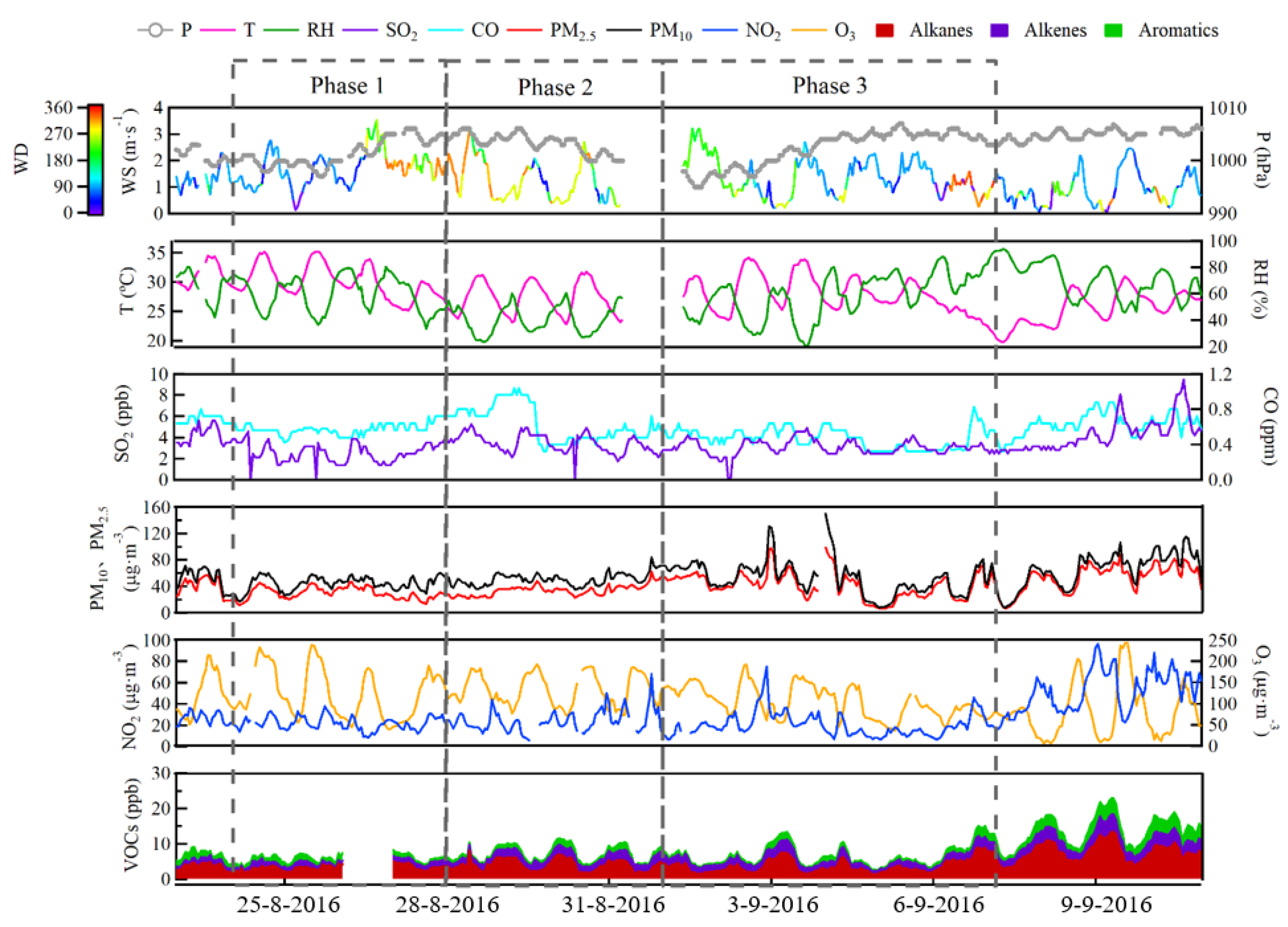
In addition to fluctuations in the intensity of anthropogenic activities, synoptic conditions play an important role in the transport and accumulation of ozone and its precursors. Figure 3 showed the time series of meteorological parameters (pressure, temperature, relative humidity, wind speed, wind direction and pressure) and pollutants (SO2, CO, PM2.5, PM10, NO2, O3 and VOCs) measured at the ZH site from 23 August to 10 September in 2016. During the control period, the variation in pollutants maintained relatively low concentration levels. During the three control phases, the hourly average mole ratios of VOCs were 5.78 ppb, 7.19 ppb and 6.54 ppb, respectively, which were 0.9–1.4 times lower than the average mole ratio after deregulation (13.65 ppb). The average concentrations of other pollutants (SO2, CO, PM2.5, PM10 and NO2) during the control period were 0.3–1.4 times lower than those after deregulation. However, as a product of the photochemical reaction, the concentrations of O3 during the three control phases were completely different, with average concentrations of 122.58 µg·m−3, 132.27 µg·m−3 and 104.73 µg·m−3. Compared with the concentration after deregulation (81.02 µg·m−3), the concentration of O3 during the control period was higher, especially during Phase 2. Combined with the meteorological parameters and the variation in other pollutants, this phenomenon was caused by synoptic conditions.
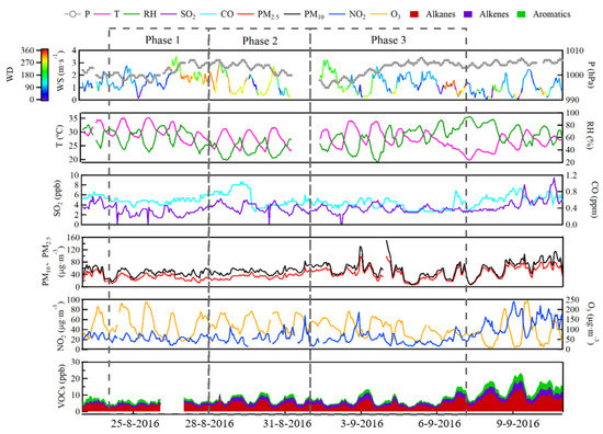
Figure 3.
Time series of meteorological parameters (pressure, wind speed, wind direction, temperature and relative humidity) and pollutants (SO2, CO, PM10, PM2.5, O3, NO2 and VOCs) measured at the ZH site.
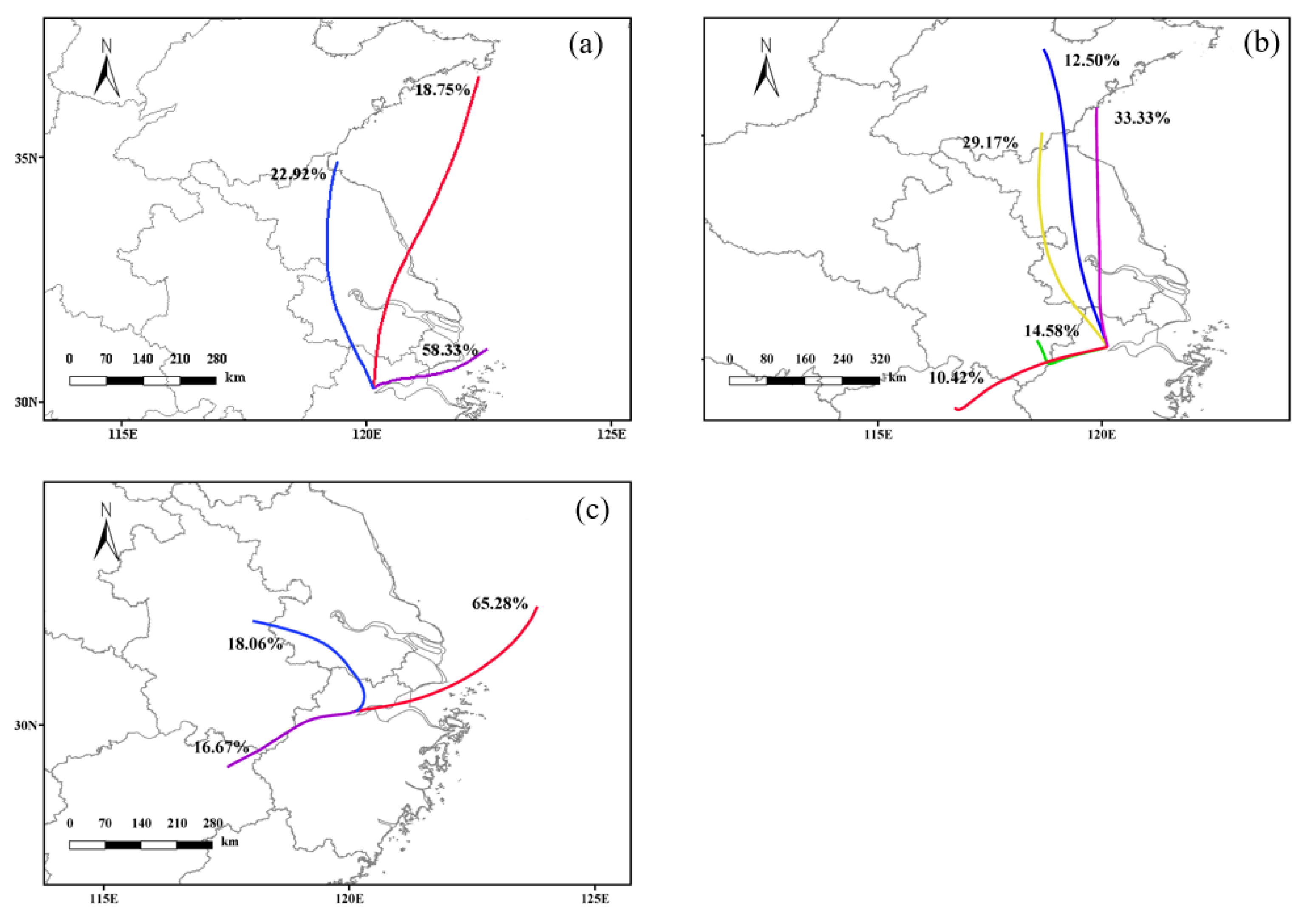
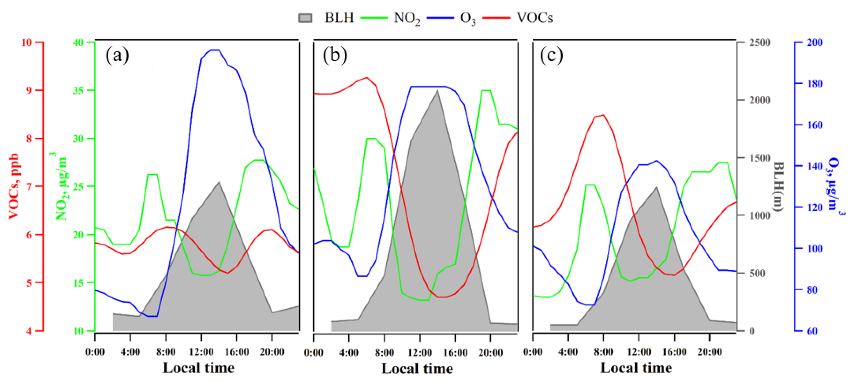
During Phase (a), the low wind speed (1.44 ± 0.61) and BLH (422.38 ± 461.40 m) on 24–25 August was not conducive to the diffusion of pollutants. In addition, the high temperature (the average maximum temperature was 34 °C) and the fine weather both were conducive to the generation of ozone. Therefore, the concentration of ozone and other pollutants during 24–25 August did not decrease obviously compared with before the control period. During 26–27 August, the wind speed increased (3.7 m·s−1), and the dominant wind direction changed to the northwest. Coupled with the decrease in temperature and the occurrence of precipitation at night on the 26th, the concentration of pollutants decreased to varying degrees. Clustered trajectories (Figure 4) showed that the airmass in Phase 1 mainly came from the Hangzhou Bay area, which was located in the core area and the strictly controlled area. Due to the control measures on primary pollutants, the concentration of ozone precursors, NO2 and VOCs, maintained low levels (Figure 5). Recent studies reported that during the G20 control period, the YRD region converted to the NOx-VOCs cooperative control region. Especially in the Hangzhou area, O3 generation was more sensitive to NOx. Therefore, the lower concentration of NO2 promoted higher O3 production. Further, the lower BLH and more photochemical activities resulted in a higher O3 increment in Phase (a).
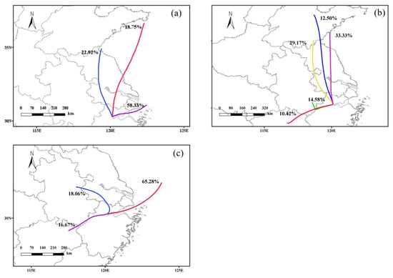
Figure 4.
Clustered trajectories (%) from different directions on different control phases (hase (a), phase (b) and phase (c)) at the ZH site.
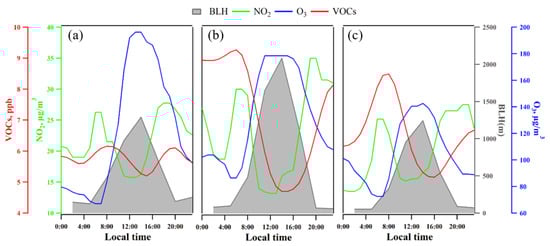
Figure 5.
Diurnal variation in boundary layer height (BLH), VOC, NO2 and O3 concentrations on different control phases: phase (a), phase (b) and phase (c).
In Phase (b), the dominant wind direction was from the northwest. The wind speed was lower than that during Phase (a). The Hangzhou area was controlled by high pressure, and the vertical diffusion capacity was weak. As can be seen in Figure 4, the northwest airflow transported the upstream pollutants to the Hangzhou area, resulting in higher concentrations of primary pollutants in Phase (b) than in Phase (a). However, the higher BLH and less photochemical activities resulted in lower O3 increment in Phase (a).
In Phase (c), the dominant wind direction on 1–3 Sep was southwest. The warm and humid airflow from the southwest was beneficial to the growth of particulate matter. Therefore, the peaks of PM2.5 and PM10 concentrations appeared on 3 Sep. During 4–6 Sep, weak precipitation appeared in the Hangzhou area, which showed an effect of wet removal of pollutants to some extent. Due to the strict joint control of the YRD regions and the clean airmass from the East Sea, the concentrations of all pollutants were lower than the first level of the air quality index (HJ633-2012). The mole ratio of VOCs reached its low point during the observation period.
As shown in Table 3, the pollutant concentrations, except for ozone, at the ZH site during the control period were lower than that after control. In addition, the pollutant concentrations at the ZH site were obviously lower than those at the DSL and YX sites during the control period. After deregulation, the concentrations of SO2, NO2, CO, PM2.5 and PM10 increased by 38.54%, 133.05%, 14.55%, 46.87% and 30.95%, respectively, compared with the control period. Due to strict measures of “coal-fired power plant capacity reduction and motor vehicle restriction etc.,” the emission of primary pollutants, such as SO2, NO2, CO, PM2.5 and PM10, was effectively controlled. This result indicated that severe control measures had favorable impacts on air quality in the Hangzhou area. In the DSL and YX areas, the concentrations of NO2 and CO increased after deregulation, by 24.77% and 1.79% in the DSL area and 17.17% and 22.95% in the YX area, respectively. Regarding the concentrations of SO2 and particulate matter, there was no significant increase after deregulation. However, the concentration of O3 decreased by 31.15%. Reduced titration by NO due to less emissions of NOx in the controlled period could be the main cause for the lower O3 in the controlled period. Ozone, as a product of photochemical reactions, was not only affected by the concentration of precursors; synoptic conditions also played an important role. Therefore, at the three sites, synoptic conditions were not conducive to the generation of ozone after deregulation. Therefore, the ozone concentration decreased after deregulation.
Table 3.
The concentrations of pollutants (SO2, NO2, CO, O3, PM2.5 and PM10) during different periods at the ZH, DSL and YX sites.
3.2. Changes in Chemical Compositions of VOCs
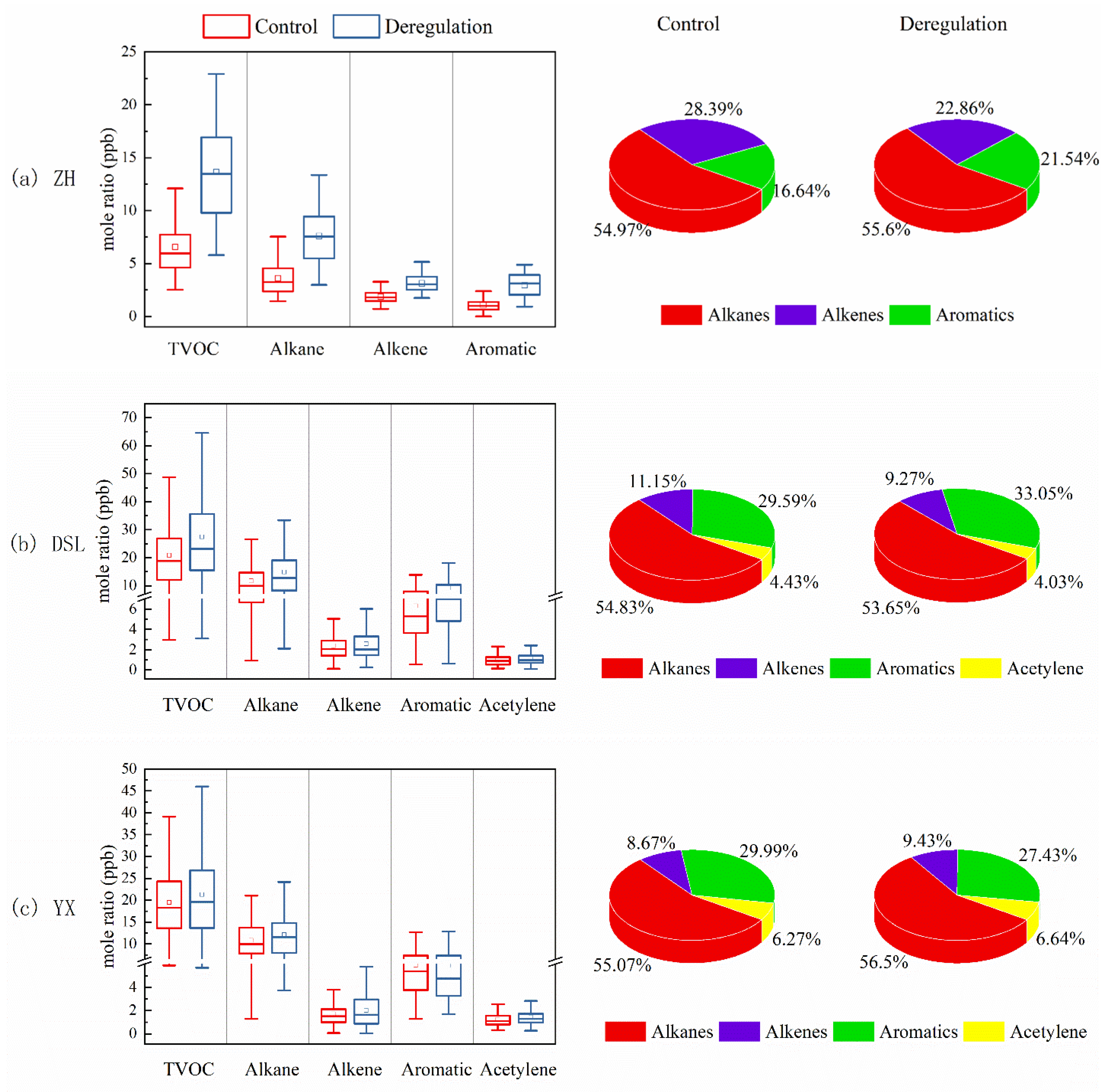
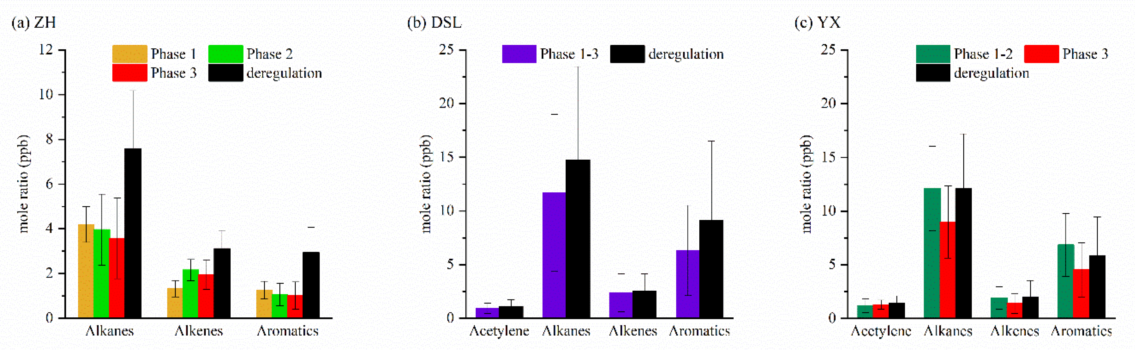
As shown on the left side of Figure 6, the mole ratios of different VOC components at the three sites all increased after deregulation. The mole ratios at the ZH site increased the most, by 108.23%, 110.62%, 67.67%, and 169.54%, respectively. The mole ratio of aromatics increased the most, followed by alkanes. As can be seen from the right side of Figure 6, the mole ratios of aromatics and alkanes also increased after deregulation, especially aromatics. The increased rate of mole ratios at the DSL site was greater than that at the YX site. After deregulation, mole ratios of TVOC, alkanes, alkenes, aromatics and acetylene increased by 31.75%, 27.15%, 8.01%, 45.13% and 18.17%, respectively, at the DSL site. The mole ratio of aromatics increased the most, followed by alkanes. Since the increase in the mole ratio of aromatics was higher than that of other components, it can be found in the proportion diagram, on the right side of Figure 6b, that the proportion of the other components reduced, except for aromatics, which increased, after deregulation. The mole ratios of the TVOC, alkanes, alkenes, aromatics and acetylene at the YX site increased to the lowest extent among the three sites, by 9.29%, 11.83%, 18.59%, −0.33% and 15.47%, respectively, compared with the control period. The mole ratios of components, except aromatics, increased after deregulation, whereas the mole ratio of aromatics decreased. Therefore, as can be seen from the right side of Figure 6c, the proportions of VOC components showed similar trends to their mole ratios. During the early control period (24–30 August) in the YX area, control measures were taken to reduce the emissions of SO2, NOx, smoke and VOCs by more than 25%. However, because the dominant wind direction in Yixing City was northwest, and the wind was relatively weak, accompanied by weak pressure, the diffusion conditions were poor [43], causing the mole ratio of VOCs to remain high in the early control period (Figure 6c).
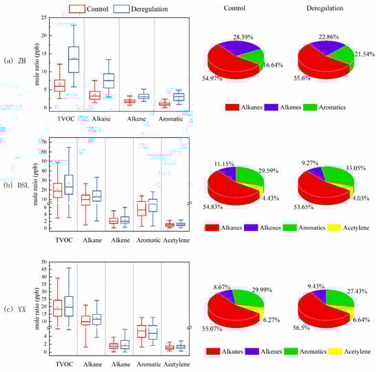
Figure 6.
The mole ratios and percentage of VOC chemical compositions during different periods at the ZH (a), DSL (b) and YX (c) sites.
3.3. Control Effect Analysis during Different Control Phases
As shown in Figure 7, to distinguish the effects of the different control periods on the mole ratios of VOCs at the three sites, we calculated the average mole ratio of VOCs in the different control periods. With the strengthening of the control measure intensity, the mole ratios of alkanes, alkenes, aromatics and acetylene decreased at the DSL and YX sites. Meanwhile, the VOC mole ratios during the control period were apparently lower than that during the deregulation period. This result confirms the effects of the stepwise control measures. The average mole ratios of VOCs in the control periods were 46.81%, 33.54% and 19.01% lower than those during deregulation at the ZH, DSL and YX sites, respectively, which was higher than the decrease in VOCs (16.4%) during the APEC meeting in Beijing [44] and that (9.83%) during the Shanghai World Expo [28]. This result indicated that the control measures in the YRD region had very obvious effects on reducing the emissions of VOCs, especially in Hangzhou.
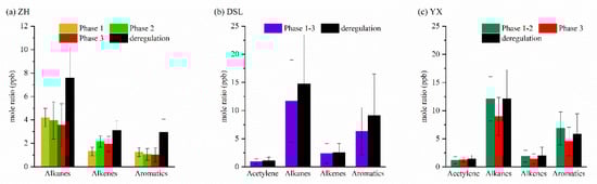
Figure 7.
The average mole ratio of VOCs in different control periods at the ZH (a), DSL (b) and YX (c) sites during the G20 summit.
As shown in Figure 7a, the mole ratio of alkenes observed at the ZH site was increased in Phase 2 compared with that in Phase 1. This was contrary to the strengthening of the control intensity. Figure 8 displayed the diurnal variation in alkenes, ethylene, propylene and isoprene. The three alkene species (ethylene, propylene and isoprene) contributed over 96% of the alkene mole ratios at the ZH site. The high mole ratios of ethylene and isoprene in Phase 2 resulted in the increasing mole ratio of alkenes. It was well acknowledged that ethylene is a product of incomplete combustion processes, especially vehicle fuel combustion [18,45]. A continuous decrease was observed from 08:00 to 16:00 LT, indicating increased photochemical removal processes. A higher concentration of NOx in Phase 2 (24.51 µg·m−3) than in Phase 1 (22.63 µg·m−3) and the morning peak of ethylene both indicated that more vehicle exhaust in Phase 2 led to the increased ethylene mole ratio. Additionally, the lower BLH at night in Phase 2 (63.57 m) compared with that in Phase 1 (176.02 m) caused the accumulation of pollutants. The diurnal variation in isoprene was controlled by plant emissions and showed one peak in the afternoon in Phase 1 and Phase 3. As shown in Figure 3, the dominant wind direction in Phase 2 was S-W. The airmass transported isoprene emitted by the forest located in the southwest of Zhejiang Province (Figure 4), which resulted in another peak in the afternoon and the increasing average mole ratio of isoprene in Phase 2.
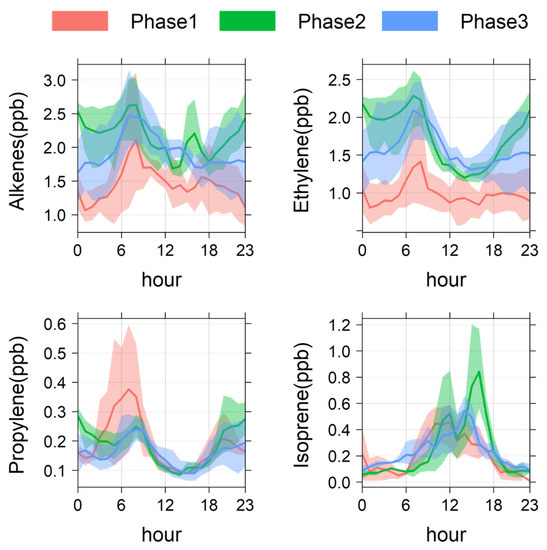
Figure 8.
Diurnal variation in alkenes, ethylene, propylene and isoprene at the ZH site. The solid line represents the mean value, and the filled area indicates the 95% confidence intervals in the mean.
3.4. Source Apportionment of VOCs
To further understand the VOC sources, five factors were resolved for VOC measurement during 23 August–15 September with PMF analysis. The number of effective samples were 336 and 96 at the ZH site, 307 and 195 at the DSL site and 299 and 188 at the YX site during the control and deregulation periods. These numbers met the condition that the span of effective samples used for PMF input data should be no less than 80 groups [46]. Because of the short data span, uncertainties regarding the PMF results were inevitable. The factor profiles of the three sites are shown in Figure S1. These factors were identified as factor 1, vehicle exhaust; factor 2, plants; factor 3, industry emissions; factor 4, fuel vaporization for the ZH and YX sites and fuel vaporization + incomplete combustion for the DSL site; factor 5, solvent usage.
The high factor loadings of long chain alkanes, ethylene, acetylene and benzene were found in factor 1. The C3-C6 alkanes usually were associated with emissions from imperfect combustion vehicular emissions [4,40]. Cai et al. [24] reported that ethylene and propylene were major species that were the product of internal combustion engines. Acetylene was an incomplete combustion tracer, while benzene was also emitted with vehicular emissions [18]. Therefore, factor 1 was attributed to vehicle exhaust.
Factor 2 exhibited a high composition of isoprene, which was mostly due to phytoncide released from plants [47]. Thus, factor 2 was as attributed to plants.
The composition for factor 3 was characterized by ethane, ethylene, propylene, acetylene and aromatics (toluene, m,p,o-xylene, m,o-ethyltoluene, trimethylbenzene, styrene). Ethylene and propylene were indicated as the raw materials or products of chemical manufacturing processes [18]. M,p,o-Xylene, trimethylbenzene and ethyltoluene were markers for solvent emission such as painting, printing and surface coating. A high proportion of styrene was detected from petroleum refining emissions. The results suggested that factor 3 is industry emissions.
At the ZH and YX sites, factor 4 was distinguished by high percentages of n-butane, isobutene, n-pentane and isopentane, with a certain amount of ethane and propane. Propane and butane are the main components of LPG/NG [4]. Ethane is associated with incomplete combustion and/or LPG/NG usage. According to a study by Sun et al. [48], isopentane and n-pentane were used as indicators for gasoline vaporization. Thus, factor 4 was attributed to fuel vaporization.
However, for the DSL site, the profile of factor 4 (see Figure S2c,d) exhibited high contributions from n-/iso-pentane, benzene and C2-C3 alkanes and alkenes. It is well acknowledged that C2-C3 are the product of incomplete combustion processes [18,45]. N-/iso-Pentane and benzene were considered as typical products of gasoline vaporization [48]. Thus, factor 4 at the DSL site was attributed to fuel vaporization + incomplete combustion.
Factor 5 was dominated by C9-C11 alkanes and aromatics (toluene, xylene, ethylbenzene). These compounds were commonly used as solvents or chemical intermediates in paints, coatings, adhesives, dyes and detergents, in addition to their use in chemical factories and fossil fuels [16,47]. Therefore, factor 5 was attributed to solvent usage.
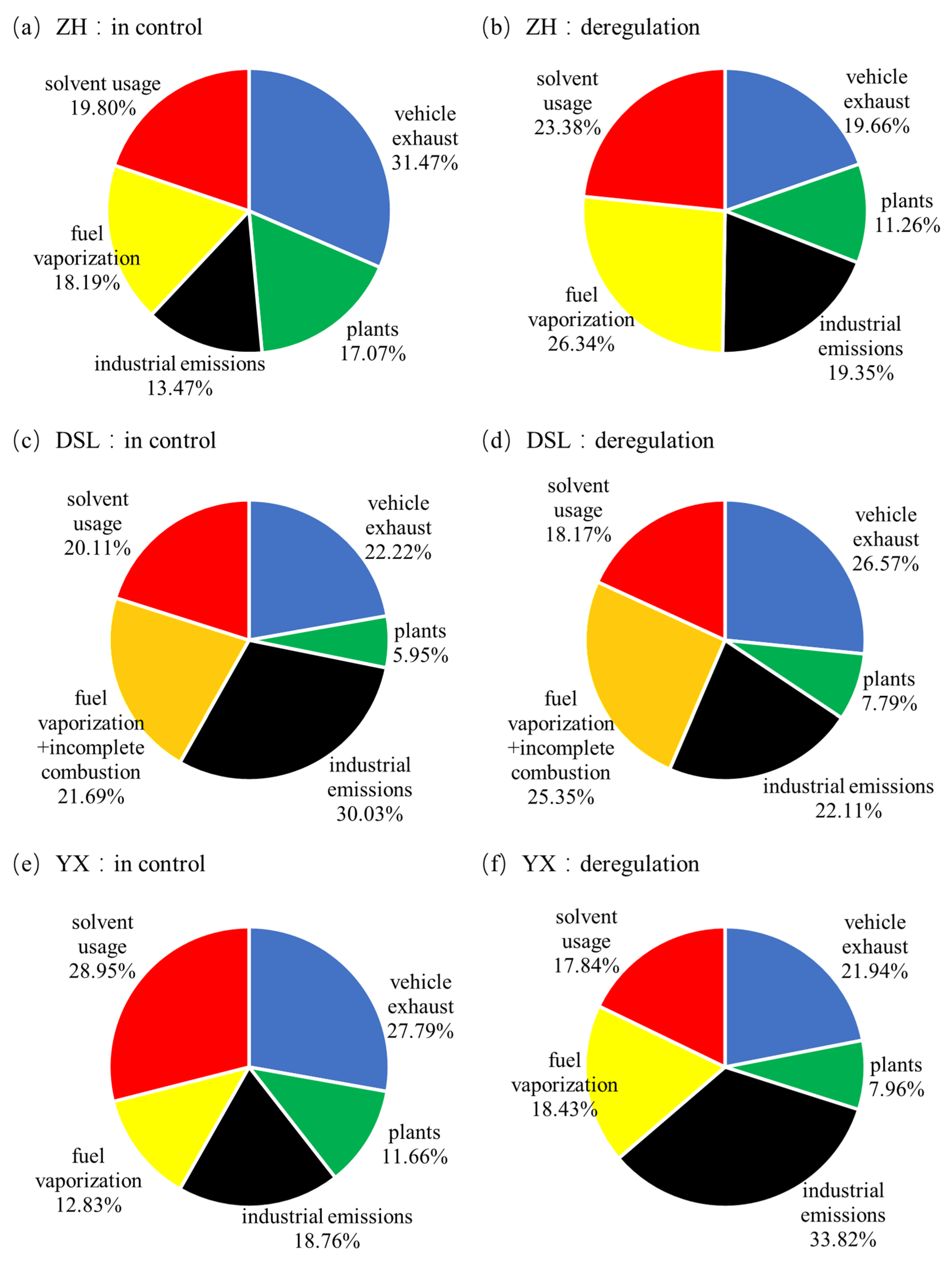
Figure 9 showed the contribution of each source of pollution to the volume fraction of VOCs as analyzed by the PMF models, in the two periods at the three sites. When ZH was deregulated, the proportion of industrial emissions sources (13.47~19.35%) and solvent usage sources (19.80~23.38%) clearly increased, which showed that the industrial emission reduction measures were effective. The proportions of vehicle exhaust (31.47~19.66%) and plant sources (17.07~11.26%) decreased because of the industrial resumption of production after deregulation. The temperature during the control period (28 ± 3 °C) was higher than that after deregulation (25 ± 3 °C), which was more conducive to for plants emissions of isoprene. In addition, in Phase 2, the ZH region may be affected by airmass transmission from forests in southwest Zhejiang (Figure 4). It may also be the reason for the higher proportion of plant sources during the control period. The source ratio of YX could also reflect the effect of the control. Industrial emissions sources (18.76~33.82%) and fuel vaporization sources (12.83~18.43%) exhibited obvious increases, while solvent usage (28.95~17.84%) and vehicle exhaust (27.79~21.94%) sources showed a decrease in the proportion due to the large increase in industrial sources. Solvent usage (28.95%) was the largest contributor during the control period, and industrial emissions (33.82%) were the largest source after deregulation. The difference in source apportionments at the DSL region during different periods cannot be adequately explained by the use of control measures. After deregulation, the proportions from industrial emissions decreased, while the proportions from plants increased.
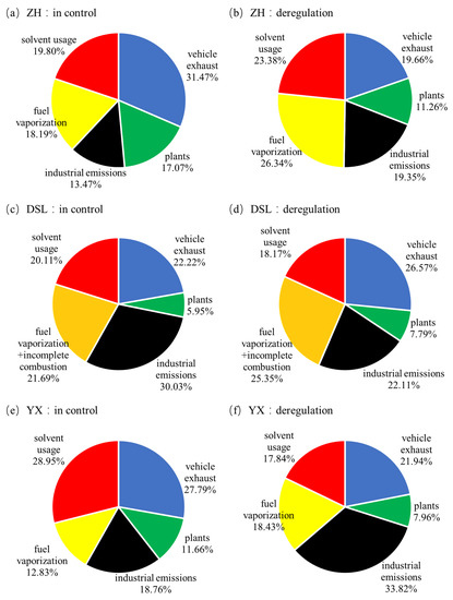
Figure 9.
Source apportionment of VOCs at the ZH ((a) in control, (b) deregulation), DSL ((c) in control, (d) deregulation) and YX ((e) in control, (f) deregulation) sites during different periods of G20 Summit.
3.5. Geographic Origin Analysis
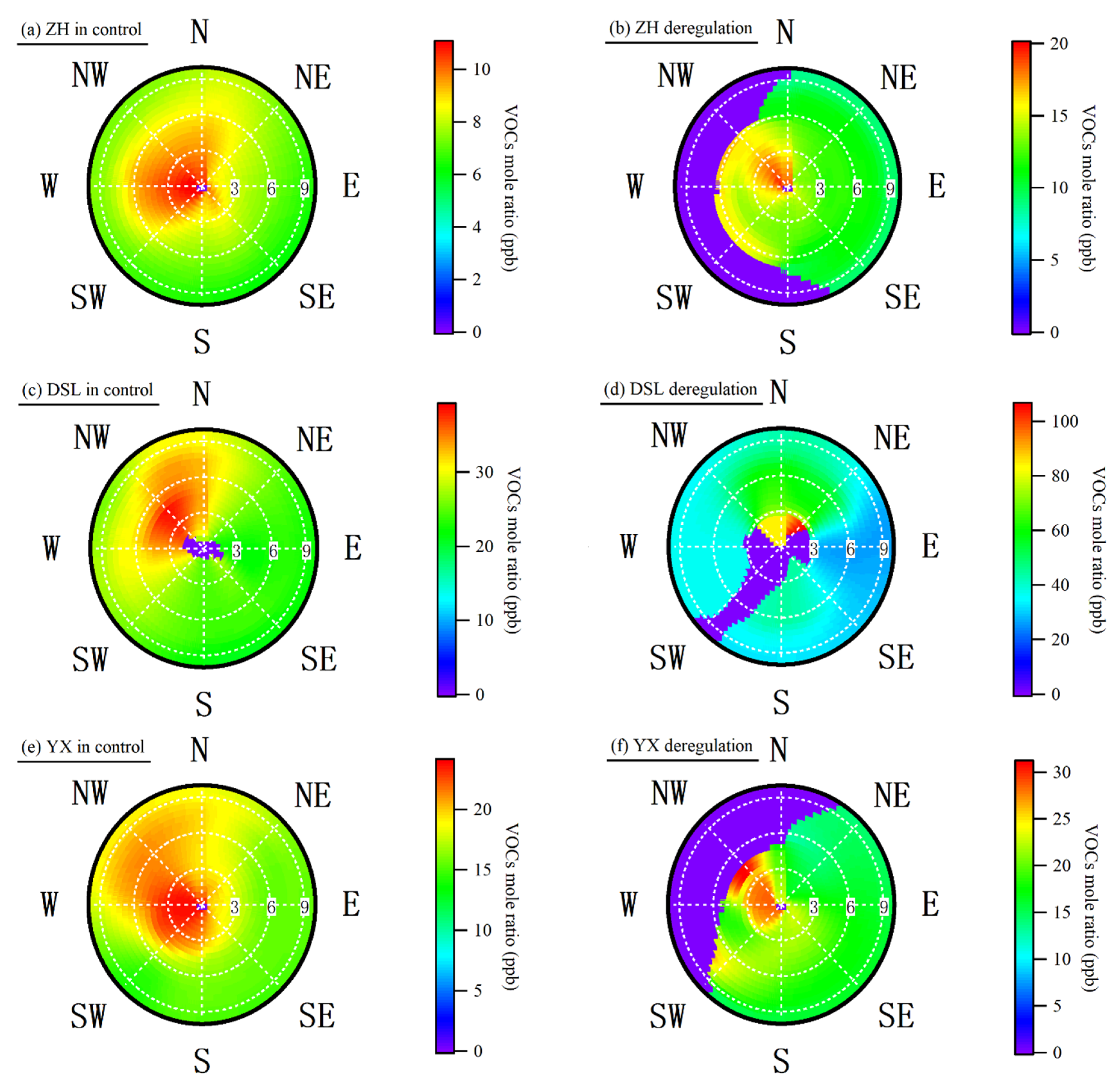
The possible local origins of VOCs were explored using the NWR method [42], as illustrated in Figure 10. As shown in Figure 10c,d, the VOC hotpots at the DSL supersite were apparently different during the control and deregulation periods. High mole ratios of VOCs were mainly associated with high wind speeds from the north-west region during the control period and from the northeast during the deregulation period (Figure 10c). The high wind speed (5~9 m·s−1) showed that VOCs measured at the DSL site during the control period were mainly from Jiangsu Province. Kunshan industrial parks were located at about 3 km to the west and about 10 km to the north of the DSL site, including electronics factories, clothing factories, paint factories, etc., which led to the increase in the proportion of solvent usage sources and industrial emission sources at the DSL site during the control period. After deregulation, the low wind speed (<3 m·s−1) illustrated that the VOCs were mainly influenced by downtown Shanghai, where vehicle exhaust and plant emissions were both abundant. Thus, the proportions from plants and vehicle exhaust increased after deregulation. Figure 10a,b shows that VOC hotpots at the ZH site were mainly in the SW-N. The corresponding wind speed (0~6 m·s−1) meant that the VOCs in the ZH region were mainly affected by local emissions and airmass transport from SW-N both during the control and deregulation period. Similar results were observed for the YX site (Figure 10e,f).
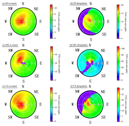
Figure 10.
Wind analysis results using non-parametric wind regression (NWR) on VOCs mole ratios measured at the ZH ((a) in control, (b) deregulation), DSL ((c) in control, (d) deregulation) and YX ((e) in control, (f) deregulation) sites during different periods of the G20 Summit.
4. Conclusions
During the G20 Summit, the average mole ratios of VOCs at the ZH, DSL and YX sites were 6.56, 21.33 and 19.62 ppb, respectively, which were lower than those (13.65, 27.72 and 21.38 ppb) after deregulation. Hangzhou implemented the most stringent control measures and obtained the lowest mole ratios of VOCs among the three cities. The total budgets of VOCs were determined by alkanes (53.65–56.5%) at the three sites, followed by alkenes (22.86–28.39%) at the ZH site and aromatics (27.43–33.05%) at the DSL and YX sites. Synoptic conditions and airmass transport played an important role in the transport and accumulation of VOCs and other pollutants, which affected the control effects.
Five factors of VOCs, namely, vehicle exhaust, plants, industrial emissions, fuel vaporization (+ incomplete combustion) and solvent usage, were identified using the PMF method for the ZH and YX sites. Factor 4 was identified as fuel vaporization + incomplete combustion at the DSL site. At the ZH site, vehicle exhaust (31.47%) and fuel vaporization (26.34%) contributed the largest proportions during the control and deregulation periods, respectively. At the YX site, solvent usage (28.95%) and industrial emission (33.82%) sources had the greatest contributions during the control and deregulation periods, respectively. The results of the source apportionment of VOCs in the control and deregulation periods from the ZH and YX regions showed the positive effects of the control measures implemented during the G20 Summit.
Additionally, NWR showed the possible geographic origins of VOCs. VOCs at the ZH and YX regions were mainly affected by local emissions and airmass transport from SW-N during both the control and deregulation periods. Regional transport decreased the proportions of industrial emissions and fuel vaporization at the DSL site. Airmasses from Jiangsu Province transported industrial emissions to the DSL region. After deregulation, a large number of VOCs that were released by vehicle exhaust and plants in downtown Shanghai were transferred to the DSL region, resulting in increased proportions from vehicle exhaust and plants.
Supplementary Materials
The following are available online at https://www.mdpi.com/article/10.3390/atmos12070928/s1, Figure S1: Qrobust, Qtrue and Qtrue/Qexcept plotted against the number of factors used in the positive matrix factorization (PMF) solution at the ZH(a), DSL(b) and YX(c) sites, Figure S2: Factor profile resolved by PMF at the ZH((a) in control,(b) deregulation), DSL((c) in control,(d) deregulation) and YX((e) in control,(f) deregulation) sites during different periods of the G20 summit, Table S1: Control measures during different control phases in Shanghai and Yixing.
Author Contributions
Conceptualization, C.C. and L.W.; methodology, Y.Z.; software, Y.Z.; validation, Y.Y., S.J. and X.Y.; formal analysis, S.Z.; investigation, Y.Q.; resources, C.C.; data curation, L.W.; writing—original draft preparation, C.C.; writing—review and editing, L.W.; visualization, Y.Z.; supervision, Y.Q.; project administration, C.C.; funding acquisition, C.C. All authors have read and agreed to the published version of the manuscript.
Funding
This research was funded by National Key Research and Development Program of China, grant number 2018YFC0209800.
Institutional Review Board Statement
Not applicable.
Informed Consent Statement
Not applicable.
Data Availability Statement
Boundary layer height (BLH) data is obtained through NOAA’s READY archived weather website (http://www.ready.noaa.gov/READYamet.php (accessed on 2 February 2021).
Acknowledgments
This work was funded by the National Key Research and Development Program of China (2018YFC0209800).
Conflicts of Interest
The authors declare no conflict of interest.
References
- Zhang, R.; Wang, G.; Guo, S.; Zamora, M.L.; Ying, Q.; Lin, Y.; Wang, W.; Hu, M.; Wang, Y. Formation of urban fine particulate matter. Chem. Rev. 2015, 115, 3803–3855. [Google Scholar] [CrossRef]
- Anand, S.S.; Philip, B.K.; Mehendale, H.M. Volatile organic compounds. In Encyclopedia of Toxicology, 3rd ed.; Wexler, P., Ed.; Academic Press: Oxford, UK, 2014; pp. 967–970. [Google Scholar]
- Durkee, J.B. Appendix b1—Chemistry of atmospheric reactions of VOCs leading to smog. In Cleaning with Solvents; Durkee, J.B., Ed.; William Andrew Publishing: Norwich, NY, USA, 2014; pp. 547–556. [Google Scholar]
- Guo, S.; Hu, M.; Zamora, M.L.; Peng, J.; Zhang, R. Elucidating severe urban haze formation in China. Proc. Natl. Acad. Sci. USA 2014, 111, 17373–17378. [Google Scholar] [CrossRef] [Green Version]
- Likun, X.; Tao, W.; Louie, P.K.K.; Luk, C.W.Y.; Blake, D.R.; Zheng, X. Increasing external effects negate local efforts to control ozone air pollution: A case study of Hong Kong and implications for other Chinese cities. Environ. Sci. Technol. 2014, 48, 10769–10775. [Google Scholar]
- Johnson, D.; Utembe, S.R.; Jenkin, M.E. Simulating the detailed chemical composition of secondary organic aerosol formed on a regional scale during the torch 2003 campaign in the southern UK. Atmos. Chem. Phys. 2006, 6, 7829–7874. [Google Scholar] [CrossRef] [Green Version]
- Huang, R.-J.; Zhang, Y.; Bozzetti, C.; Ho, K.-F.; Cao, J.-J.; Han, Y.; Daellenbach, K.R.; Slowik, J.G.; Platt, S.M.; Canonaco, F.; et al. High secondary aerosol contribution to particulate pollution during haze events in China. Nature 2014, 514, 218–222. [Google Scholar] [CrossRef] [Green Version]
- Shrivastava, M.; Cappa, C.; Fan, J.H.; Goldstein, A.; Guenther, A.L.; Jimenez, J.; Kuang, C.; Laskin, A.; Martin, S.; Lee Ng, N.; et al. Recent advances in understanding secondary organic aerosol: Implications for global climate forcing. Rev. Geophys. 2017, 55, 277–585. [Google Scholar] [CrossRef] [Green Version]
- Zhang, Y.; Tang, L.; Sun, Y.; Favez, O.; Canonaco, F.; Albinet, A.; Couvidat, F.; Liu, D.; Jayne, J.T.; Zhuang, W. Limited formation of isoprene epoxydiols-derived secondary organic aerosol under nox-rich environments in eastern China. Cell. Immunol. 2017, 44, 2035–2043. [Google Scholar] [CrossRef] [Green Version]
- Min, S.; Yuanhang, Z.; Limin, Z.; Xiaoyan, T.; Jing, Z.; Liuju, Z.; Boguang, W. Ground-level ozone in the pearl river delta and the roles of VOC and NOx in its production. J. Environ. Manag. 2009, 90, 512–518. [Google Scholar]
- Zhang, Q.; Yuan, B.; Shao, M.; Wang, X.; Lu, S.; Lu, K.; Wang, M.; Chen, L.; Chang, C.C.; Liu, S.C. Variations of ground-level O3 and its precursors in Beijing in summertime between 2005 and 2011. Atmos. Chem. Phys. 2014, 14, 6089–6101. [Google Scholar] [CrossRef] [Green Version]
- Ke, L.; Jacob, D.J.; Liao, H.; Shen, L.; Bates, K.H. Anthropogenic drivers of 2013–2017 trends in summer surface ozone in China. Proc. Natl. Acad. Sci. USA 2019, 116, 422–427. [Google Scholar]
- Li, L.; Xie, S.; Zeng, L.; Wu, R.; Li, J. Characteristics of volatile organic compounds and their role in ground-level ozone formation in the Beijing-Tianjin-Hebei region, China. Atmos. Environ. 2015, 113, 247–254. [Google Scholar] [CrossRef]
- An, J.; Zhu, B.; Wang, H.; Li, Y.; Lin, X.; Yang, H. Characteristics and source apportionment of VOCs measured in an industrial area of Nanjing, Yangtze River Delta, China. Atmos. Environ. 2014, 97, 206–214. [Google Scholar] [CrossRef]
- Li, L.; An, J.Y.; Shi, Y.Y.; Zhou, M.; Yan, R.S.; Huang, C.; Wang, H.L.; Lou, S.R.; Wang, Q.; Lu, Q.; et al. Source apportionment of surface ozone in the Yangtze River Delta, China in the summer of 2013. Atmos. Environ. 2016, 144, 194–207. [Google Scholar] [CrossRef]
- Shao, P.; An, J.; Xin, J.; Wu, F.; Wang, J.; Ji, D.; Wang, Y. Source apportionment of VOCs and the contribution to photochemical ozone formation during summer in the typical industrial area in the Yangtze River Delta, China. Atmos. Res. 2016, 176–177, 64–74. [Google Scholar] [CrossRef]
- Tang, J.H.; Chan, L.Y.; Chan, C.Y.; Li, Y.S.; Chang, C.C.; Liu, S.C.; Wu, D.; Li, Y.D. Characteristics and diurnal variations of NMHCs at urban, suburban, and rural sites in the Pearl River Delta and a remote site in south China. Atmos. Environ. 2007, 41, 8620–8632. [Google Scholar] [CrossRef]
- Liu, Y.; Shao, M.; Fu, L.; Lu, S.; Zeng, L.; Tang, D. Source profiles of volatile organic compounds (VOCs) measured in China: Part I. Atmos. Environ. 2008, 42, 6247–6260. [Google Scholar] [CrossRef]
- Cheng, H.R.; Guo, H.; Saunders, S.M.; Lam, S.H.M.; Jiang, F.; Wang, X.M.; Simpson, I.J.; Blake, D.R.; Louie, P.K.K.; Wang, T.J. Assessing photochemical ozone formation in the Pearl River Delta with a photochemical trajectory model. Atmos. Environ. 2010, 44, 4199–4208. [Google Scholar] [CrossRef] [Green Version]
- Ling, Z.H.; Guo, H.; Cheng, H.R.; Yu, Y.F. Sources of ambient volatile organic compounds and their contributions to photochemical ozone formation at a site in the Pearl River Delta, southern China. Environ. Pollut. 2011, 159, 2310–2319. [Google Scholar] [CrossRef]
- Song, Y.; Shao, M.; Liu, Y.; Lu, S.; Kuster, W.; Goldan, P.; Xie, S. Source apportionment of ambient volatile organic compounds in Beijing. Environ. Sci. Technol. 2007, 41, 4348–4353. [Google Scholar] [CrossRef] [PubMed]
- Wang, B.; Shao, M.; Lu, S.H.; Yuan, B.; Zhao, Y.; Wang, M.; Zhang, S.Q.; Wu, D. Variation of ambient non-methane hydrocarbons in Beijing city in summer 2008. Atmos. Chem. Phys. Discuss. 2010, 10, 5911–5923. [Google Scholar] [CrossRef] [Green Version]
- Yuan, B.; Shao, M.; Lu, S.; Wang, B. Source profiles of volatile organic compounds associated with solvent use in Beijing, China. Atmos. Environ. 2010, 44, 1919–1926. [Google Scholar] [CrossRef]
- Cai, C.; Geng, F.; Tie, X.; Yu, Q.; An, J. Characteristics and source apportionment of VOCs measured in Shanghai, China. Atmos. Environ. 2010, 44, 5005–5014. [Google Scholar] [CrossRef]
- Wang, H.; Qiao, Y.; Chen, C.; Lu, J.; Dai, H.; Qiao, L.; Lou, S.; Huang, C.; Li, L.; Jing, S.; et al. Source profiles and chemical reactivity of volatile organic compounds from solvent use in Shanghai, China. Aerosol Air Qual. Res. 2014, 14, 301–310. [Google Scholar] [CrossRef] [Green Version]
- Yang, X.X.; Tang, L.L.; Hu, B.X.; Zhou, H.C.; Hua, Y.; Qin, W.; Chen, W.T.; Cui, Y.H.; Jiang, L. Sources apportionment of volatile organic compounds vocs in summertime Nanjing and their potential contribution to secondary organic aerosols (SOA). China Environ. Sci. 2016, 36, 2896–2902. [Google Scholar]
- Shao, M.; Lu, S.; Liu, Y.; Xie, X.; Chang, C.; Huang, S.; Chen, Z. Volatile organic compounds measured in summer in beijing and their role in ground-level ozone formation. J. Geophys. Res. Atmos. 2009, 114. [Google Scholar] [CrossRef]
- Wang, H.L.; Chen, C.H.; Huang, H.Y.; Wang, Q.; Chen, Y.R.; Huang, C.; Li, L.I.; Zhang, G.F.; Chen, M.H.; Lou, S.R. Emission strength and source apportionment of volatile organic compounds in shanghai during 2010 EXPO. Huanjing Kexue 2012, 33, 4151–4158. [Google Scholar]
- Geng, C.; Wang, J.; Yin, B.; Zhao, R.; Bai, Z. Vertical distribution of volatile organic compounds conducted by tethered balloon in the Beijing-Tianjin-Hebei region of China. J. Environ. Sci. 2020, 95, 121–129. [Google Scholar] [CrossRef] [PubMed]
- Yu, H.; Dai, W.; Ren, L.L.; Liu, D.; Yan, X.T.; Xiao, H.; He, J.; Xu, H.H. The effect of emission control on the submicron particulate matter size distribution in Hangzhou during the 2016 G20 summit. Aerosol Air Qual. Res. 2018, 18, 2038–2046. [Google Scholar] [CrossRef] [Green Version]
- Zhou, D.R.; Tian, X.D.; Cai, Z.; Wang, X.Y.; Li, Y.; Liu, Y.; Jiang, F. Evaluation of ozone change and control effects in Yangtze River Delta region during G20 summit. Environ. Monit. China 2020, 36, 41–49. [Google Scholar]
- Gros, V.; Gaimoz, C.; Herrmann, F.; Custer, T.; Williams, J.; Bonsang, B.; Sauvage, S.; Locoge, N.; D’Argouges, O.; Sarda-esteve, R.; et al. Volatile organic compounds source apportionment in Paris in spring 2007. EGU General Assembly. 2009, 11, 12418. [Google Scholar]
- Lyu, X.P.; Chen, N.; Guo, H.; Zhang, W.H.; Wang, N.; Wang, Y.; Liu, M. Ambient volatile organic compounds and their effect on ozone production in Wuhan, central China. Sci. Total Environ. 2016, 541, 200–209. [Google Scholar] [CrossRef]
- Wang, Y.; Zhang, X.; Draxler, R.R. TrajStat: GIS-based software that uses various trajectory statistical analysis methods to identify potential sources from long-term air pollution measurement data. Environ. Model. Softw. 2009, 24, 938–939. [Google Scholar] [CrossRef]
- Squizzato, S.; Masiol, M. Application of meteorology based methods to determine local and external contributions to particulate matter pollution: A case study in Venice (Italy). Atmos. Environ. 2015, 119, 69–81. [Google Scholar] [CrossRef]
- Zheng, H.; Kong, S.F.; Xing, X.L.; Mao, Y.; Hu, T.P.; Ding, Y.; Li, G.; Liu, D.T.; Li, S.L.; Qi, S.H. Monitoring of volatile organic compounds (VOCs) from an oil and gas station in northwest China for 1 year. Atmos. Chem. Phys. 2018, 18, 4567–4595. [Google Scholar] [CrossRef] [Green Version]
- Paatero, P.; Tapper, U. Positive matrix factorization: A non-negative factor model with optimal utilization of error estimates of data values. Environmetrics 2010, 5, 111–126. [Google Scholar] [CrossRef]
- Norris, G.; Duvall, R.; Brown, S.; Bai, S. EPA Positive Matrix Factorization (PMF) 5.0 Fundamentals and User Guide. Available online: https://www.epa.gov/sites/production/files/2015-02/documents/pmf_5.0_user_guide.pdf (accessed on 12 July 2021).
- Brown, S.G.; Frankel, A.; Hafner, H.R. Source apportionment of VOCs in the Los Angeles area using positive matrix factorization. Atmos. Environ. 2007, 41, 227–237. [Google Scholar] [CrossRef]
- Zhang, Y.; Li, R.; Fu, H.; Zhou, D.; Chen, J. Observation and analysis of atmospheric volatile organic compounds in a typical petrochemical area in Yangtze River Delta, China. J. Environ. Sci. 2018, 71, 233–248. [Google Scholar] [CrossRef]
- Henry, R.; Norris, G.A.; Vedantham, R.; Turner, J.R. Source region identification using kernel smoothing. Environ. Sci. Technol. 2009, 43, 4090–4097. [Google Scholar] [CrossRef]
- Petit, J.E.; Favez, O.; Albinet, A.; Canonaco, F. A user-friendly tool for comprehensive evaluation of the geographical origins of atmospheric pollution: Wind and trajectory analyses. Environ. Model. Softw. 2017, 88, 183–187. [Google Scholar] [CrossRef] [Green Version]
- Shi, W.K.; Qian, Y.H.; Bian, Z.M.; Pan, X.; Li, X.Z.; Xie, W.P. Ozone and VOCs characteristics and control effect in Yixing during the G20 Summit. Sichuan Environ. 2019, 38, 92–97. [Google Scholar]
- Gan, Y.; Wei, W.; Zhao-Feng, L.V.; Cheng, S.Y.; Yue, L.I. Characteristics of VOCs in Beijing urban area during APEC period and its verification for VOCs emission inventory. China Environ. Sci. 2016, 36, 1297–1304. [Google Scholar]
- Goldan, P.D.; Parrish, D.D.; Kuster, W.C.; Mckeen, S.A.; Fehsenfeld, F.C. Airborne measurements of isoprene, CO, and anthropogenic hydrocarbons and their implications. J. Geophys. Res. Atmos. 2000, 105, 9091–9106. [Google Scholar] [CrossRef]
- Gao, S.; Cui, H.X.; Fu, Q.Y.; Tian, X.Y.; Fang, F.; Yi, X.W.; Gao, S.; Cui, H.X.; Fu, Q.Y.; Tian, X.Y. Characteristics and source apportionment of VOCs of high pollution process at chemical industrial area in winter of China. Environ. Sci. 2016, 37, 4094–4102. [Google Scholar]
- Wu, F.; Yu, Y.; Sun, J.; Zhang, J.; Wang, J.; Tang, G.; Wang, Y. Characteristics, source apportionment and reactivity of ambient volatile organic compounds at Dinghu Mountain in Guangdong Province, China. Sci. Total Environ. 2016, 548–549, 347–359. [Google Scholar] [CrossRef]
- Sun, J.; Wu, F.; Hu, B.; Tang, G.; Wang, Y. VOC characteristics, emissions and contributions to SOA formation during hazy episodes. Atmos. Environ. 2016, 141, 560–570. [Google Scholar] [CrossRef]

Publisher’s Note: MDPI stays neutral with regard to jurisdictional claims in published maps and institutional affiliations. |
© 2021 by the authors. Licensee MDPI, Basel, Switzerland. This article is an open access article distributed under the terms and conditions of the Creative Commons Attribution (CC BY) license (https://creativecommons.org/licenses/by/4.0/).