
Chinese Sunspot Drawings and Their Digitizations-(VI) Extreme Value Theory Applied to the Sunspot Number Series from the Purple Mountain Observatory

 ,
, 
Abstract
:1. Introduction
2. Data and Methods
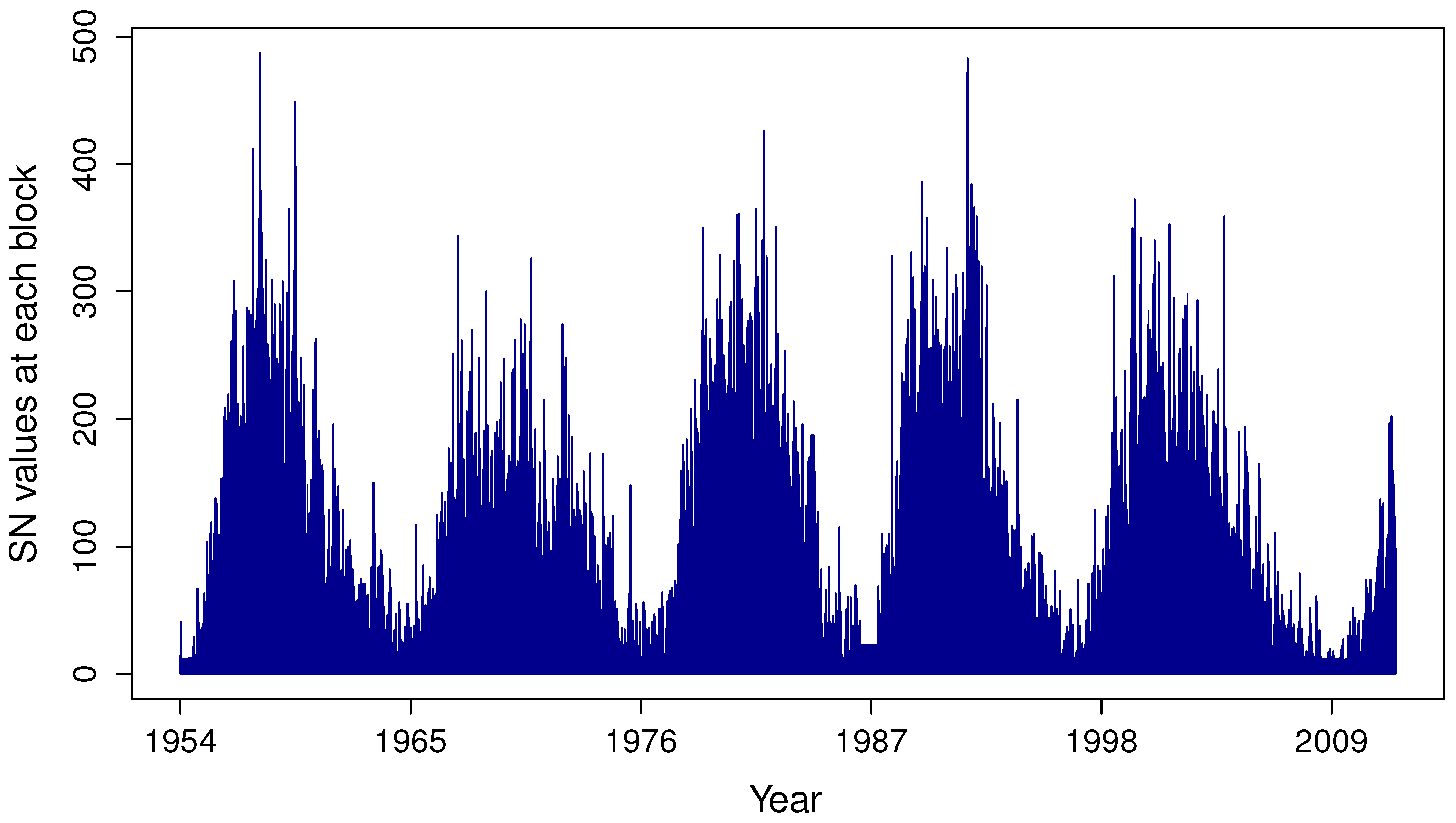
2.1. Data
2.2. Methods
3. Results
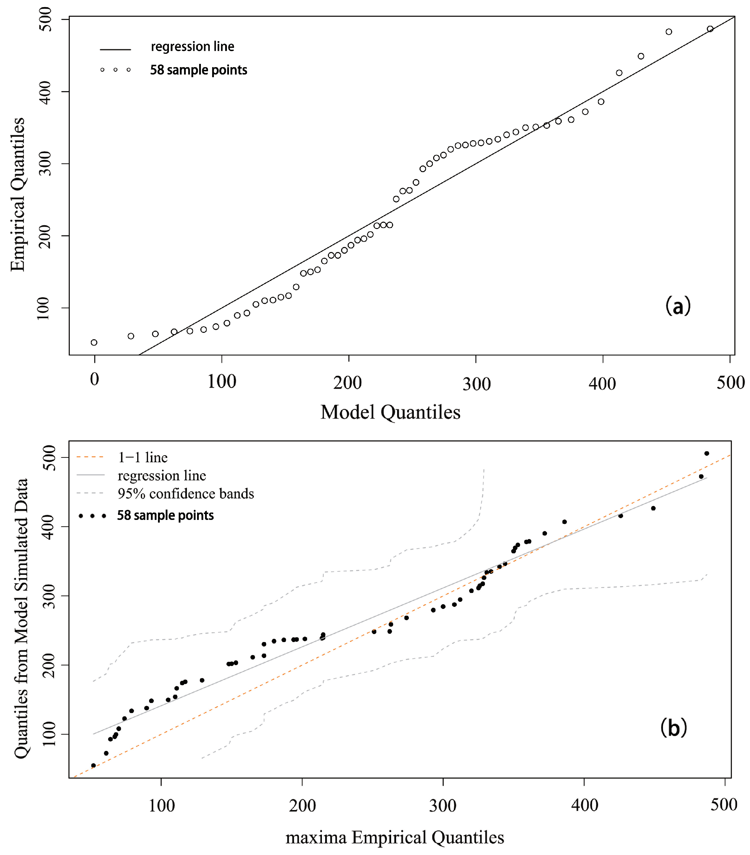
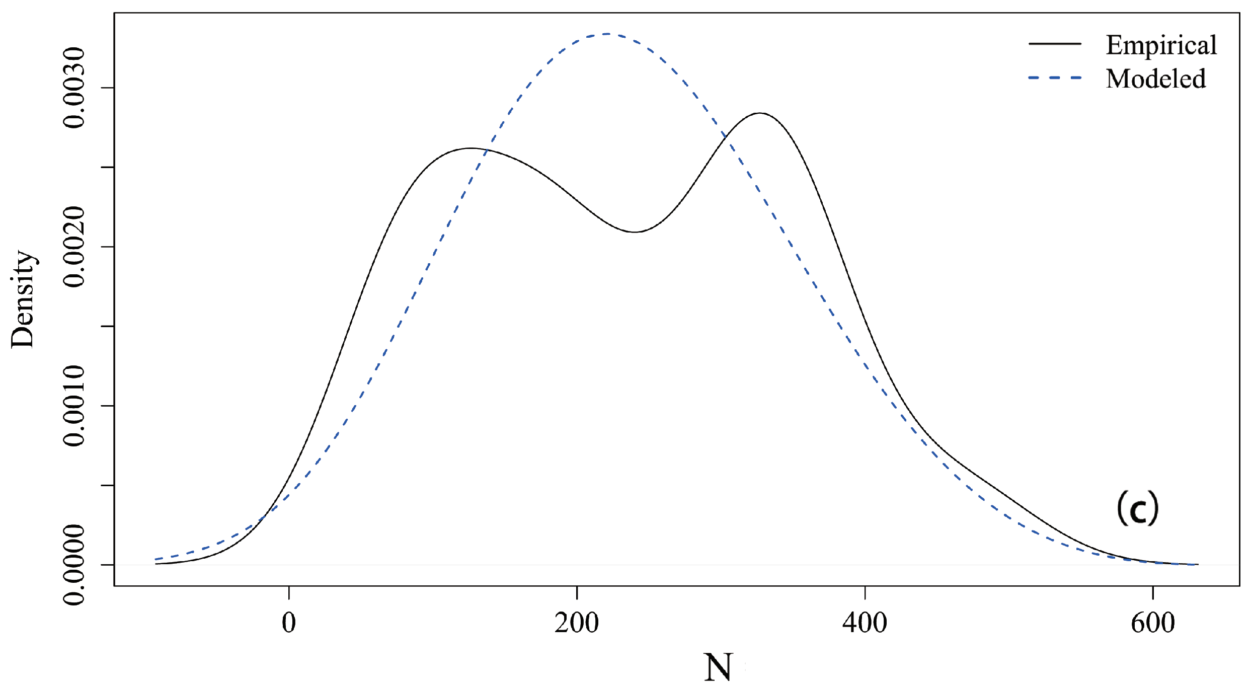
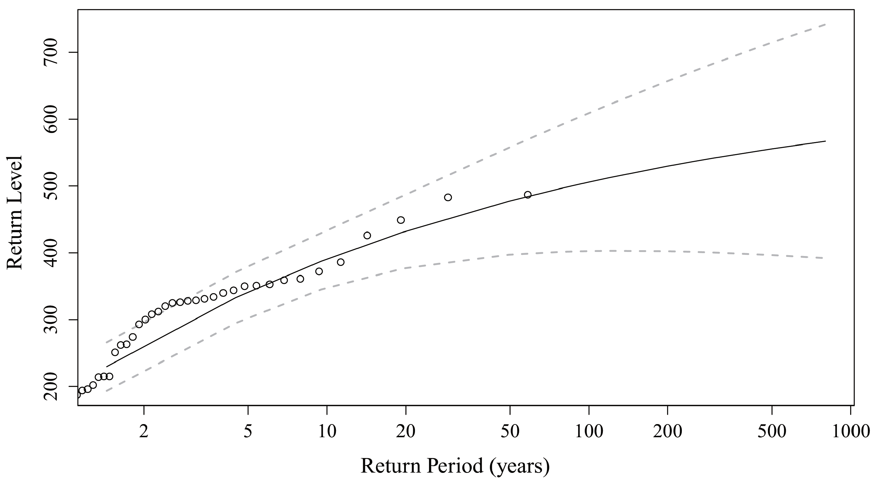
3.1. Block Maxima Approach
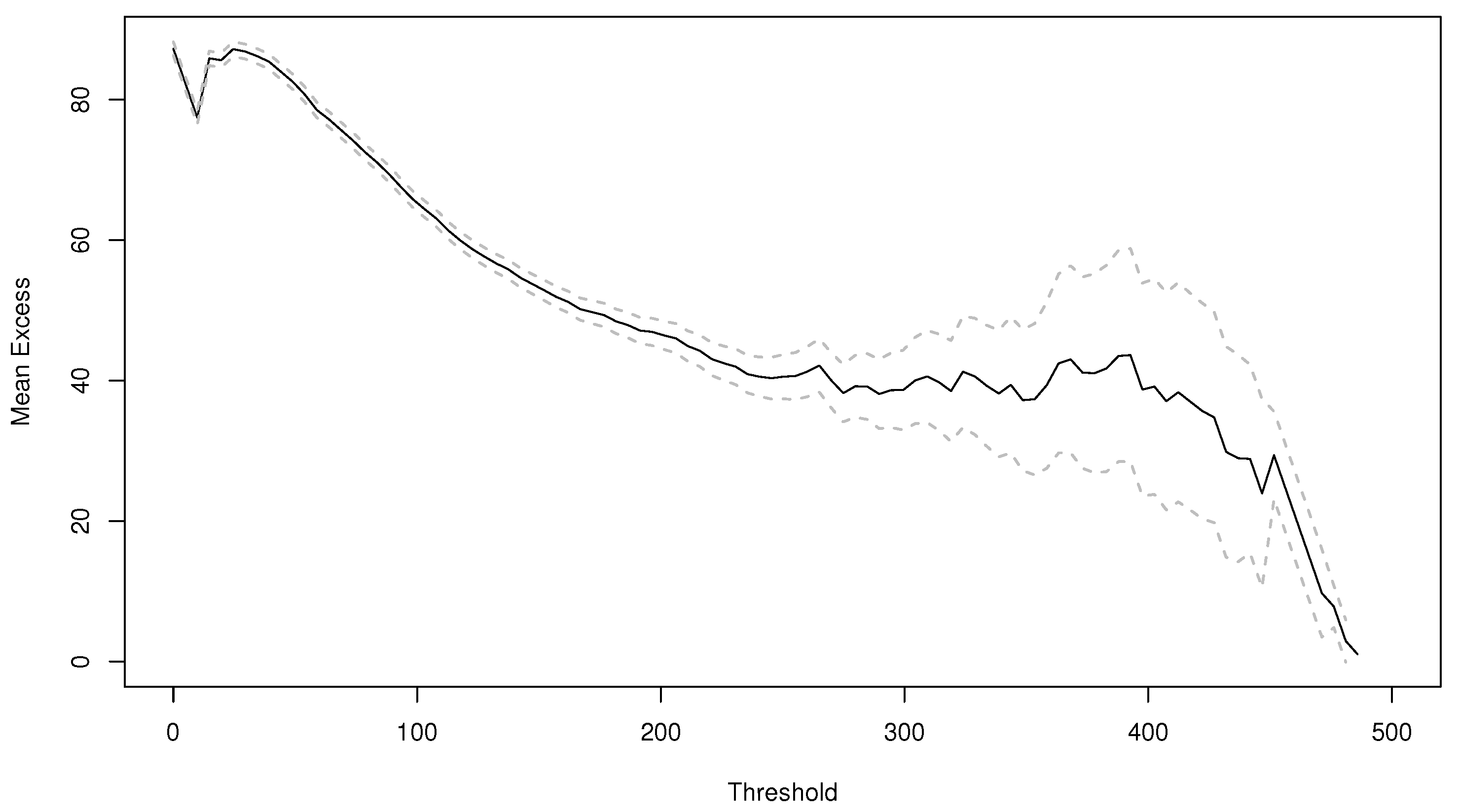
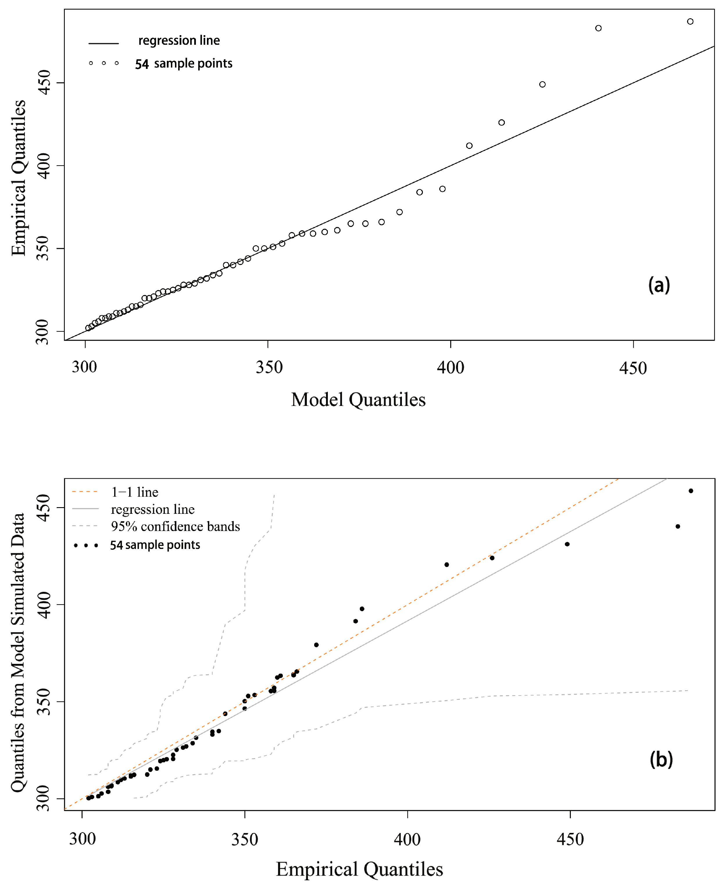
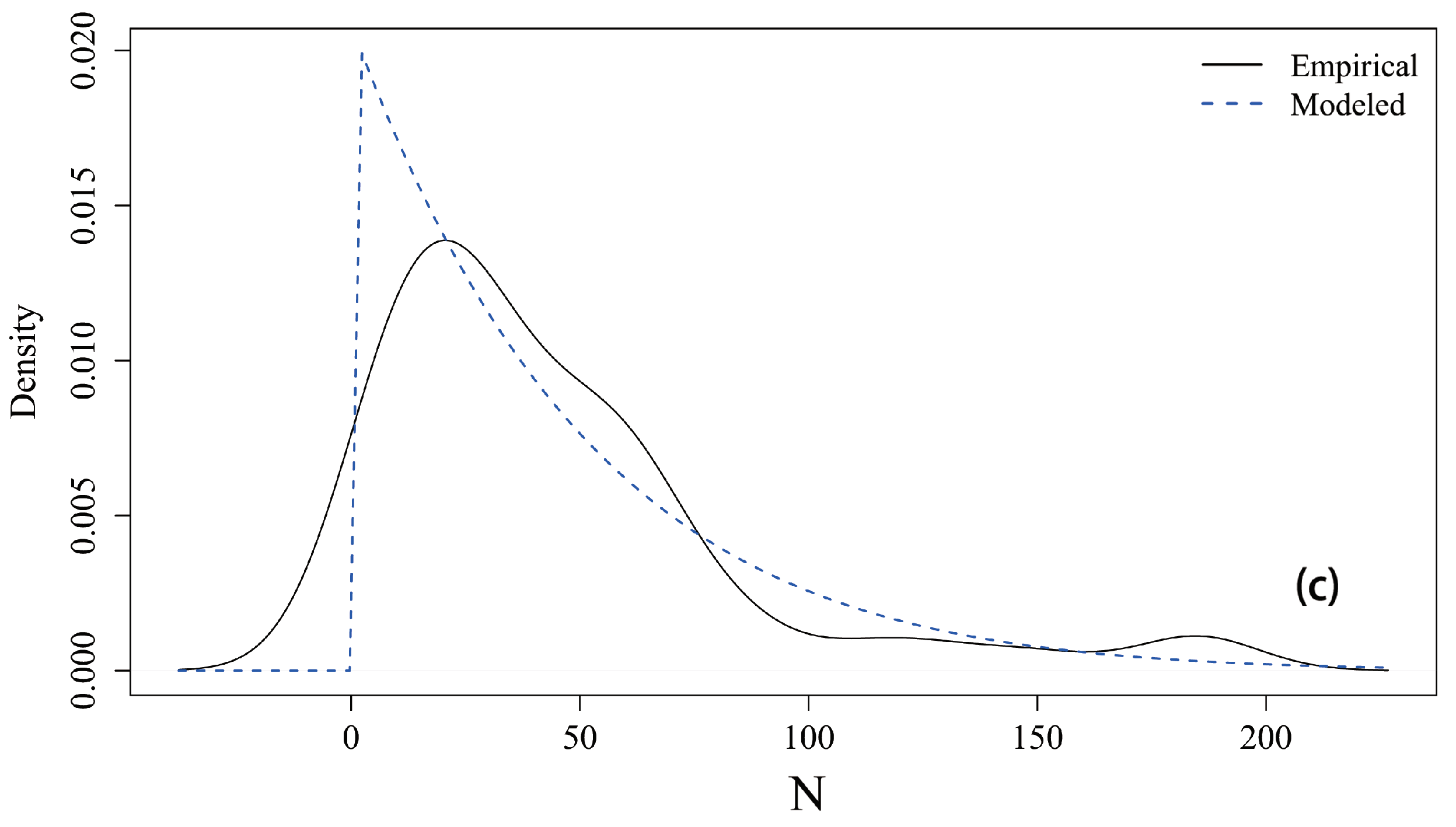
3.2. Peaks-Over-Threshold Approach
4. Discussion and Conclusions
Author Contributions
Funding
Institutional Review Board Statement
Informed Consent Statement
Data Availability Statement
Acknowledgments
Conflicts of Interest
References
- Deng, L.H.; Li, B.; Zheng, Y.F.; Cheng, X.M. Relative phase analyses of 10.7 cm solar radio flux with sunspot numbers. New Astron. 2013, 23, 1–5. [Google Scholar] [CrossRef]
- Pala, Z.; Atici, R. Forecasting Sunspot Time Series Using Deep Learning Methods. Sol. Phys. 2019, 294, 50. [Google Scholar] [CrossRef]
- Deng, L.H.; Li, B.; Xiang, Y.Y.; Dun, G.T. Multi-scale analysis of coronal Fe XIV emission: The role of mid-range periodicities in the Sun-heliosphere connection. J. Atmos. Sol.-Terr. Phys. 2015, 122, 18–25. [Google Scholar] [CrossRef]
- Deng, L.H.; Fei, Y.; Deng, H.; Mei, Y.; Wang, F. Spatial distribution of quasi-biennial oscillations in high-latitude solar activity. Mon. Not. R. Astron. Soc. 2020, 494, 4930–4938. [Google Scholar] [CrossRef]
- Charbonneau, P. Dynamo models of the solar cycle. Living Rev. Sol. Phys. 2020, 17, 4. [Google Scholar] [CrossRef]
- Vaquero, J.M.; Vázquez, M. Scientific Data Extracted from Historical Documents. In The Sun Recorded through History; Springer: New York, NY, USA, 2009; p. 361. [Google Scholar]
- Deng, L.-H.; Qu, Z.-Q.; Yan, X.-L.; Wang, K.R. Phase analysis of sunspot group numbers on both solar hemispheres. Res. Astron. Astrophys. 2013, 13, 104–114. [Google Scholar] [CrossRef]
- Lefèvre, L. Detailed Analysis of Solar Data Related to Historical Extreme Geomagnetic Storms: 1868–2010. Sol. Phys. 2016, 291, 1483–1531. [Google Scholar] [CrossRef] [Green Version]
- Coles, S. An Introduction to Statistical Modeling of Extreme Values; Springer: London, UK, 2001. [Google Scholar]
- Nogaj, M.; Yiou, P.; Parey, S.; Malek, F. Amplitude and frequency of temperature extremes over the North Atlantic region. Geophys. Res. Lett. 2006, 33, L10801. [Google Scholar] [CrossRef]
- Coelho, C.A.S.; Ferro, C.A.T.; Stephenson, D.B.; Steinskog, D.J. Methods for Exploring Spatial and Temporal Variability of Extreme Events in Climate Data. J. Clim. 2008, 21, 2072. [Google Scholar] [CrossRef] [Green Version]
- Acero, F.J.; García, J.A.; Gallego, M.C. Peaks-over-Threshold Study of Trends in Extreme Rainfall over the Iberian Peninsula. J. Clim. 2011, 24, 1089–1105. [Google Scholar] [CrossRef]
- Acero, F.J.; García, J.A.; Gallego, M.C.; Parey, S.; Dacunha-Castelle, D. Trends in summer extreme temperatures over the Iberian Peninsula using nonurban station data. J. Geophys. Res. (Atmos.) 2014, 119, 39–53. [Google Scholar] [CrossRef]
- Gilli, M.; Këllezi, E. An Application of Extreme Value Theory for Measuring Financial Risk. Comput. Econ. 2006, 27, 207–228. [Google Scholar] [CrossRef] [Green Version]
- Castillo, E.; Hadi, A.S.; Balakrishnan, N.; Sarabia, J.M. Extreme Value and Related Models with Applications in Engineering and Science; Wiley-Interscience: New York, NY, USA, 2004. [Google Scholar]
- Bhavsar, S.P.; Barrow, J.D. First ranked galaxies in groups and clusters. Mon. Not. R. Astron. Soc. 1985, 213, 857–869. [Google Scholar] [CrossRef]
- Bernstein, J.P.; Bhavsar, S.P. Models for the magnitude-distribution of brightest cluster galaxies. Mon. Not. R. Astron. Soc. 2001, 322, 625–630. [Google Scholar] [CrossRef] [Green Version]
- Deng, L.H.; Zhang, X.J.; Deng, H.; Mei, Y.; Wang, F. Systematic regularity of solar coronal rotation during the time interval 1939–2019. Mon. Not. R. Astron. Soc. 2020, 491, 848–857. [Google Scholar] [CrossRef]
- Siscoe, G.L. On the statistics of the largest geomagnetic storms per solar cycle. J. Geophys. Res. 1976, 81, 4782. [Google Scholar] [CrossRef]
- Asensio Ramos, A. Extreme value theory and the solar cycle. Astron. Astrophys. 2007, 472, 293–298. [Google Scholar] [CrossRef] [Green Version]
- Acero, F.J.; Carrasco, V.M.S.; Gallego, M.C.; García, J.A.; Vaquero, J.M. Extreme Value Theory and the New Sunspot Number Series. Astrophys. J. 2017, 839, 98. [Google Scholar] [CrossRef]
- Elvidge, S.; Angling, M.J. Using Extreme Value Theory for Determining the Probability of Carrington-Like Solar Flares. Space Weather 2018, 16, 417–421. [Google Scholar] [CrossRef]
- Acero, F.J.; Gallego, M.C.; García, J.A.; Usoskin, I.G.; Vaquero, J.M. Extreme Value Theory Applied to the Millennial Sunspot Number Series. Astrophys. J. 2018, 853, 80. [Google Scholar] [CrossRef] [Green Version]
- Acero, F.J.; Vaquero, J.M.; Gallego, M.C.; García, J.A. Extreme Value Theory Applied to the Daily Solar Radio Flux at 10.7 cm. Sol. Phys. 2019, 294, 67. [Google Scholar] [CrossRef]
- Love, J.J. Some Experiments in Extreme-Value Statistical Modeling of Magnetic Superstorm Intensities. Space Weather 2020, 18, e02255. [Google Scholar] [CrossRef] [Green Version]
- Lin, G.H. Chinese Sunspot Drawings and Their Digitization— (I) Parameter Archives. Sol. Phys. 2019, 294, 79. [Google Scholar] [CrossRef] [Green Version]
- Sun, X.B.; Zheng, S.; He, H.L.; Zeng, S.G. System Difference Analysis for the 55 Years’ Hand-drawing Sunspot Data of Purple Mountain Observatory. Acta Astron. Sin. 2019, 60, 55–63. [Google Scholar]
- Wan, M.; Zeng, S.-G.; Zheng, S.; Lin, G.-H. Chinese sunspot drawings and their digitization—(III) quasi-biennial oscillation of the hand-drawn sunspot records. Res. Astron. Astrophys. 2020, 20, 190. [Google Scholar] [CrossRef]
- Clette, F.; Svalgaard, L.; Vaquero, J.M.; Cliver, E.W. Revisiting the Sunspot Number. A 400-Year Perspective on the Solar Cycle. Space Sci. Rev. 2014, 186, 35–103. [Google Scholar] [CrossRef] [Green Version]
- Kharin, V.V.; Zwiers, F.W. Changes in the Extremes in an Ensemble of Transient Climate Simulations with a Coupled Atmosphere-Ocean GCM. J. Clim. 2000, 13, 3760–3788. [Google Scholar] [CrossRef]
- García, J.A.; Gallego, M.C.; Serrano, A.; Vaquero, J.M. Trends in Block-Seasonal Extreme Rainfall over the Iberian Peninsula in the Second Half of the Twentieth Century. J. Clim. 2007, 20, 113–130. [Google Scholar] [CrossRef]
- Ferreira, A.; Haan, L.D. On the block maxima method in extreme value theory: PWM estimators. Ann. Stat. 2013, 43, 276–298. [Google Scholar] [CrossRef] [Green Version]
- Heristchi, D.; Mouradian, Z. The global rotation of solar activity structures. Astron. Astrophys. 2009, 497, 835–841. [Google Scholar] [CrossRef]
- Lee, J.N.; Shindell, D.T.; Hameed, S. The Influence of Solar Forcing on Tropical Circulation. J. Clim. 2009, 22, 5870. [Google Scholar] [CrossRef]
- Kukoleva, A.A.; Kononova, N.K.; Krivolutskii, A.A. Manifestation of the Solar Cycle in the Circulation Characteristics of the Lower Atmosphere in the Northern Hemisphere. Geomagn. Aeron. 2018, 58, 775–783. [Google Scholar] [CrossRef]
- Guttu, S. Impacts of UV Irradiance and Medium-Energy Electron Precipitation on the North Atlantic Oscillation during the 11-Year Solar Cycle. Atmosphere 2021, 12, 1029. [Google Scholar] [CrossRef]
- Deng, L.H.; Li, B.; Xiang, Y.Y.; Dun, G.T. Comparison of Chaotic and Fractal Properties of Polar Faculae with Sunspot Activity. Astron. J. 2016, 151, 2. [Google Scholar] [CrossRef]
- Wu, S.-S.; Qin, G. Predicting Sunspot Numbers for Solar Cycles 25 and 26. arXiv 2021, arXiv:2102.06001. [Google Scholar]
- Kakad, B.; Kumar, R.; Kakad, A. Randomness in Sunspot Number: A Clue to Predict Solar Cycle 25. Sol. Phys. 2020, 295, 88. [Google Scholar] [CrossRef]
- Sarp, V.; Kilcik, A.; Yurchyshyn, V.; Rozelot, J.P.; Ozguc, A. Prediction of solar cycle 25: A non-linear approach. Mon. Not. R. Astron. Soc. 2018, 481, 2981–2985. [Google Scholar] [CrossRef] [Green Version]
- Li, F.Y.; Kong, D.F.; Xie, J.L.; Xiang, N.B.; Xu, J.C. Solar cycle characteristics and their application in the prediction of cycle 25. J. Atmos. Sol.-Terr. Phys. 2018, 181, 110–115. [Google Scholar] [CrossRef]


| Location () [95% CI] | Scale () [95% CI] | Shape () [95% CI] |
|---|---|---|
| 189.74 [155.49, 224.01] | 113.78 [87.64, 139.92] | −0.24 [−0.49, 0.01] |
| 19 Year-RL |
|---|
| 420.84 (371.82, 463.88) |
| Scale () [95% CI] | Shape () [95% CI] |
|---|---|
| 47.98 [30.39, 65.57] | −0.08 [−0.33, 0.18] |
| 19 Year-RL |
|---|
| 420.99 (393.49, 461.14) |
| Method/Model | Time of Predicting | Trend of Solar Activity | Reference |
|---|---|---|---|
| BMA, POT | SC 25 | stronger | Our works |
| TMLP-E models | SC 25 and 26 | Similar | [38] |
| A model based on Shannon entropy | SC 25 | stronger | [39] |
| Non-linear prediction algorithm | SC 25 | stronger | [40] |
| The bimodal distribution | SC 25 | stronger | [41] |
Publisher’s Note: MDPI stays neutral with regard to jurisdictional claims in published maps and institutional affiliations. |
© 2021 by the authors. Licensee MDPI, Basel, Switzerland. This article is an open access article distributed under the terms and conditions of the Creative Commons Attribution (CC BY) license (https://creativecommons.org/licenses/by/4.0/).
Share and Cite
Chen, Y.-Q.; Zheng, S.; Xiao, Y.-S.; Zeng, S.-G.; Zhou, T.-H.; Lin, G.-H. Chinese Sunspot Drawings and Their Digitizations-(VI) Extreme Value Theory Applied to the Sunspot Number Series from the Purple Mountain Observatory. Atmosphere 2021, 12, 1176. https://doi.org/10.3390/atmos12091176
Chen Y-Q, Zheng S, Xiao Y-S, Zeng S-G, Zhou T-H, Lin G-H. Chinese Sunspot Drawings and Their Digitizations-(VI) Extreme Value Theory Applied to the Sunspot Number Series from the Purple Mountain Observatory. Atmosphere. 2021; 12(9):1176. https://doi.org/10.3390/atmos12091176
Chicago/Turabian StyleChen, Yan-Qing, Sheng Zheng, Yan-Shan Xiao, Shu-Guang Zeng, Tuan-Hui Zhou, and Gang-Hua Lin. 2021. "Chinese Sunspot Drawings and Their Digitizations-(VI) Extreme Value Theory Applied to the Sunspot Number Series from the Purple Mountain Observatory" Atmosphere 12, no. 9: 1176. https://doi.org/10.3390/atmos12091176
APA StyleChen, Y.-Q., Zheng, S., Xiao, Y.-S., Zeng, S.-G., Zhou, T.-H., & Lin, G.-H. (2021). Chinese Sunspot Drawings and Their Digitizations-(VI) Extreme Value Theory Applied to the Sunspot Number Series from the Purple Mountain Observatory. Atmosphere, 12(9), 1176. https://doi.org/10.3390/atmos12091176