Identification of SUHI in Urban Areas by Remote Sensing Data and Mitigation Hypothesis through Solar Reflective Materials

Abstract

The urban heat island (UHI) is an increasingly widespread phenomenon of concern to the wellbeing and the health of populations living in urban environments. The SUHI (Surface UHI) is directly related to UHI and influences its extension and intensity. Satellite images in the thermal infrared spectral region can be used to identify and study the SUHI. In this work, Landsat 8 TIR images were acquired to study the SUHI of a medium-sized municipality of the Po valley in the northern part of Italy. An additional Worldview 3 satellite image was used to classify the study area and retrieve the surface albedo of building roofs. Using the Local Climate Zone approach, existing roof materials were virtually replaced by solar reflective materials, and the mitigation potential of the SUHI and the UHI was quantified. This virtual scenario shows a decrease in the overheating of building roofs with respect to the ambient temperature of up to 33% compared to the current situation in the industrial areas. Focusing on UHI intensity, the air temperature decrease could be up to 0.5 °C.

1. Introduction

The global population is increasingly moving from small rural areas to cities. In 2018, 55.3% of the world’s population lived in cities, and the threshold of 60% should be reached by 2030. There were 548 cities with at least one million inhabitants in 2018, but that could rise to 706 in 2030 [1,2]. Over-urbanization, combined with the growing problems related to climate change and global warming, will lead in the near future to the worsening of many of the social, health, and environmental negative effects in urban areas [3,4].

A main problem of cities is the Urban Heat Island (UHI), a phenomenon which is well-known and widely reported in the literature by the scientific community [5,6,7,8]. The UHI is a microclimatic phenomenon occurring in metropolitan areas and consists of a significant temperature increase in urban areas compared to the neighboring peripheral and rural areas [9]. The UHI is mainly due to manmade surfaces, such as concrete and asphalt, which adsorb more solar radiation than natural surfaces such as vegetation and bare soils. Furthermore, urban impervious surfaces, such as asphalt and concrete, show very low evapotranspiration, resulting in a low dissipation of energy as latent heat [10,11]. This effect is more pronounced in summer and results in a significant difference in mean temperature between the city and the suburbs [12]. Heat stored during the day is slowly dissipated by radiation, starting in the late afternoon and during the night, while in rural areas, bare soils and vegetation dissipate heat faster [13].

In the scientific literature, a distinction is made between the Surface Urban Heat Island (SUHI) and the (atmospheric) Urban Heat Island (UHI). The latter represents the difference in air temperature between the urban and rural areas while the former refers to ground temperatures. The SUHI is usually at a maximum during the day, when the sun heats the surfaces, and decreases at night; the UHI, on the other hand, reaches its maximum during the night when the air above the city warms up due to the dissipation of heat from the urban surfaces [14,15,16,17]. Thus, surface overheating (SUHI) leads to an increase in the UHI phenomenon caused by the heat transfer between the surface and the atmosphere above. The effects due to the SUHI and the UHI have direct repercussions on air pollution, on the demand for energy and water, and on a population’s health (especially the weakest part of the population) [18,19]. For these reasons, it is increasingly necessary and urgent to design cities following strategies aimed at limiting the heat accumulation [20]. As anthropogenic heat release and urban morphology are driving factors for the UHI [21], mitigation actions need to be performed locally, taking into account the land use (the presence of impervious surfaces in residential, commercial, and industrial areas) and also architectural constraints due to the cultural heritage of the city. In this framework, the Local Climate Zone (LCZ) approach developed by Stewart and Oke [22,23] could be useful in helping to identify areas of intervention. Mitigation actions include the use of solar reflective materials (the so-called “cool materials”) [24,25]. They have a surface albedo value higher than that of the traditional materials and thus represent a countermeasure to urban warming by increasing the solar reflectance of urban surfaces and, therefore, urban solar heat gain [26,27,28].

Remote sensing data can provide valuable support for both the identification of SUHIs and the urban surface classification and analysis [18,19,20,29,30,31,32,33,34]. Images acquired in the thermal infrared spectral region (TIR), at wavelengths from 8 to 14 μm, allow one to obtain maps of Land Surface Temperature (LST) and therefore to study and analyze the SUHI [30,31,32,33]. The LST retrieved from the Landsat 8 TIR images is certainly suitable for the assessment of SUHIs at an urban scale; nevertheless, due to the low spatial resolution, it is not useful for the estimation of the single roof temperature [26].

However, images acquired in the visible (VIS)–near infrared (NIR) (0.4 to 1.4 µm) and with high spatial resolution (less than a few meters) allow one to classify urban surfaces and retrieve the surface albedo [35], which is an important parameter that influences SUHIs and UHIs. The albedo, or solar reflectance, of a surface is the hemispherical reflection of solar radiation integrated over the solar spectrum from 0.3 to 2.5 µm [36]. The short-wave infrared region (SWIR) also contributes to the albedo calculation, but the satellite sensors currently available do not have spatial resolutions suitable to distinguish between objects such as roofs and roads at an urban scale. Nevertheless, several models have been proposed in the literature to compute the albedo using only VIS–NIR data [37,38,39]. Several methods reported in the literature [40,41] allow the calculation of the maximum temperature of each building roof using the albedo, the surface cover type (classification), and the meteorological data of the area.

In this work, remote sensing is used for the characterization of urban surfaces and the detection of hot areas (i.e., areas showing high mean surface temperature) in order to analyze the SUHI and the UHI. The TIR images acquired by TIRS/Landsat 8 satellite sensor [42] have been used to identify the SUHI of the municipality of Reggio Emilia, a medium-sized city of the Po Valley in the northern part of Italy. The analysis focuses on some particular industrial areas, identified using the LCZ approach and used in support of the identification of local actions to mitigate the SUHI and the UHI phenomenon.

Impervious surface areas with high surface temperatures were selected as target areas for this study. Moreover, some rural areas, with low surface temperatures, were used for comparison. A Worldview 3 satellite image was used for the classification of the surface type and for the calculation of the surface albedo.

After the SUHI analysis, the urban surface characterization and the building roof surface temperature calculation, some mitigation actions based on solar reflective materials are suggested. Two scenarios are built in the LCZ considered: the first one assumes the complete replacement of the current building roofs with solar reflective materials immediately after their installation; the second is the same scenario but after a few years, with solar reflective materials that have undergone an aging process [43,44,45]. The benefits achieved by these scenarios are assessed in terms of the increase in the surface albedo, the decrease in the building roof surface temperature (mitigation action for the SUHI) and the air temperature decrease for the UHI.

2. Materials and Methods

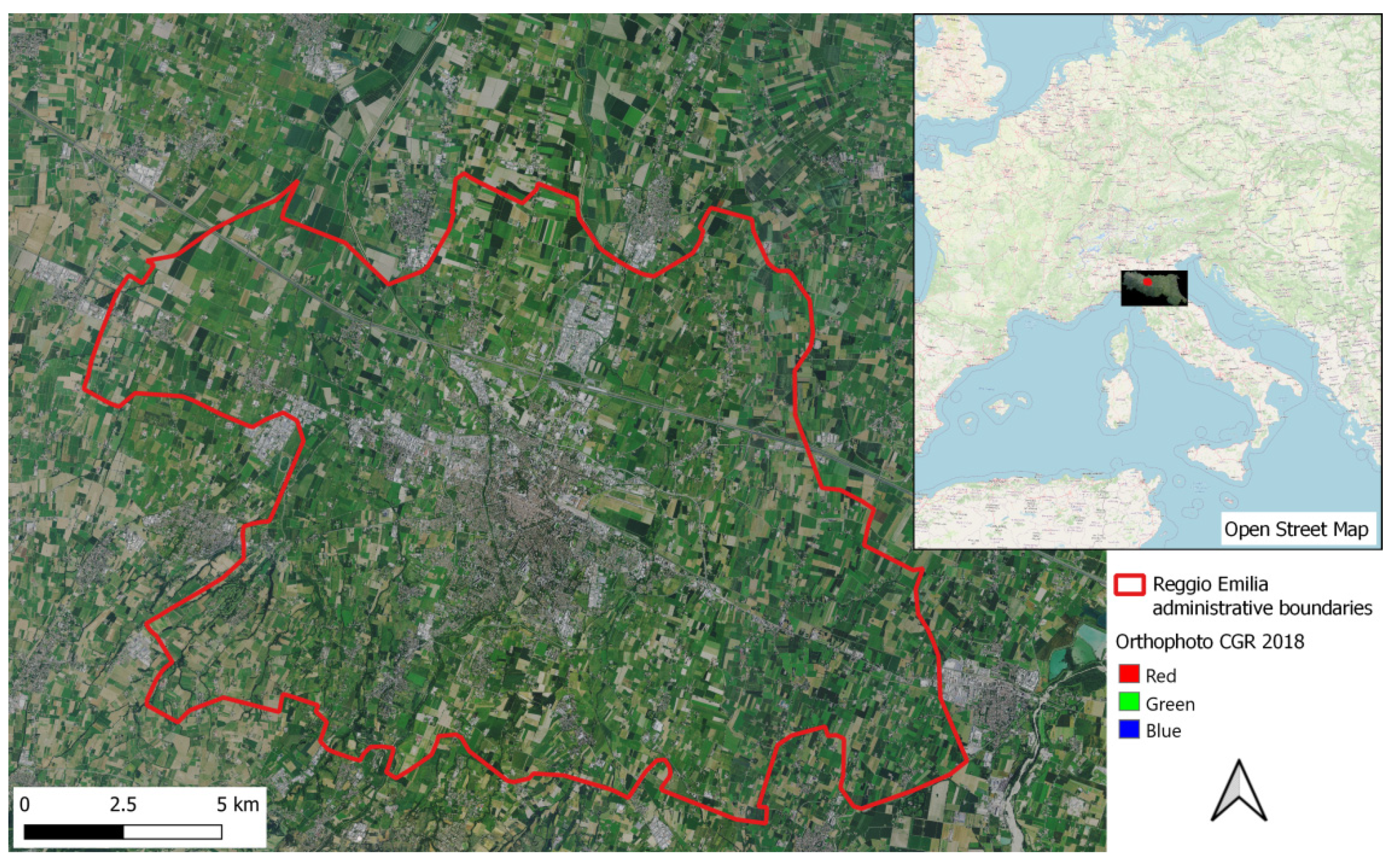
2.1. Study Area

The study area of this work is the municipality of Reggio Emilia (Figure 1). Reggio Emilia has 160,000 inhabitants and covers an area of 231 km². The city is located in the Po Valley, halfway between the Po river and the Apennine mountains [46]. High population density, industrialization processes, and intensive agriculture are characteristics of the Po Valley of which Reggio Emilia is a part [47]. This is an area characterized by temperate continental climatic conditions. The summers are hot and muggy, and the winters are cold and humid. The rainfall is distributed throughout the year, but the rainiest seasons are autumn and spring, while the driest ones are winter and summer [48,49,50]. The winters are typically characterized by the thermal inversion phenomenon, with an accumulation of pollutants near to the soil surface; the autumns and winters are frequently foggy, mainly in the plains [50].

The meteorological data of the area were measured by the “Reggio Emilia San Lazzaro” meteorological station (Lat. 44.69, Lon. 10.67), located inside the San Lazzaro university campus and part of the network of measurement stations of the Geophysical Observatory of the University of Modena and Reggio Emilia [51].

Reggio Emilia has been divided into 63 municipal districts by the local administration. These areas have very different sizes: there are many districts in the historic center with small dimensions, while in the rural areas they cover large portions of the territory.

2.2. Local Climate Zones (LCZs) Approach

The LCZs were defined by Stewart and Oke as “Regions of uniform surfaces cover, structure, material, and human activity that span hundreds of meters to several kilometers in horizontal scale” [22]. The LCZs were introduced here to assess the potentiality of mitigation actions for SUHIs and, consequently, for UHIs at a local scale. In Italian historical cities such as Reggio Emilia, the urbanization process throughout the years caused an irregular growth of the city that has resulted in commercial/industrial areas close to the city center or generally mixed with residential areas. Mitigation strategies must consider the replacement of roofs with different solar reflective materials depending on the area of the city. City center roofs are almost exclusively made of clay tiles because they are part of the cultural heritage and therefore it is very difficult to consider a change in the color of the materials. On the other hand, flat roofs on residential or commercial/industrial buildings are suitable for replacement with cool roofs. As these zones are often contiguous to the city center, mitigation effects provided by new roofs can lend benefits to the surrounding areas. For these reasons, it is preferable to act considering single areas rather than the entire urban area. Thus, after the SUHI identification by the Landsat 8 TIR images, some LCZs in which it is possible and advantageous to consider the replacement of roofs will be considered. Some rural areas will also be considered for comparison.

2.3. Data Set

For this study, both satellite images and vector files were used. In particular, the satellite data from Landsat 8 were used to retrieve the LST maps, while an image from the Worldview3 satellite allowed us to classify urban surfaces and to calculate the surface albedo. The municipality of Reggio Emilia and the topographic geodatabase of the cartographic archive of Emilia Romagna Region (Geoportale-Emilia Romagna) provided vector shapefiles and high resolution orthoimages, which were used as a support for the image processing and classification.

2.3.1. Landsat 8 Images

Landsat 8 is an American satellite for Earth observation, in operation since 2013 and developed and managed by NASA and USGS (United States Geological Survey) [42]. The spacecraft voyages at an altitude of 705 km, completing one orbit every 99 min and repeating the cycle every 16 days. It moves along a near polar orbit, flying over every point of the Earth at 10:00 a.m. +/− 15 min (helio synchronous orbit).

The satellite is equipped with two sensors: the OLI (Operational Land Imager) collects image data from bands in the VIS–NIR spectral region; the TIRS (Thermal Infrared Sensor) operates with two bands in the TIR spectral region. The OLI bands have a spatial resolution of 30 m; the TIRS bands have a spatial resolution of 100 m (but the images are resampled at 30 m). Bands features are shown in

Table 1. Landsat 8 bands technical features.

Bands	Wavelength (Micrometers)	Resolution (Meters)
Band 1—Coastal	0.43–0.45	30
Band 2—Blue	0.45–0.51	30
Band 3—Green	0.53–0.59	30
Band 4—Red	0.64–0.67	30
Band 5—Near infrared (NIR)	0.85–0.88	30
Band 6—SWIR 1	1.57–1.65	30
Band 7—SWIR 2	2.11–2.29	30
Band 8—Panchromatic	0.50–0.68	15
Band 9—Cirrus	1.36–1.38	30
Band 10—Thermal Infrared (TIR)	10.60–11.19	100
Band 11—Thermal Infrared (TIR)	11.50–12.51	100

. Both the OLI and the TIRS bands were used to calculate the LST and the vegetation information of the study area.

A time series of TIR satellite images is required to achieve a full assessment of the time and space variability of the SUHI because the latter is driven by climate and meteorological conditions. The years from 2016 to 2021 were considered for this study and, because the UHI shows its effects particularly during spring and summer, only the months from May to September of every year were analyzed. During the cold months, the UHI has a lower intensity and it results in a free heat source [46,52,53]. First of all, the Landsat 8 images available in the period of interest were considered. The first selection rejected all the cloudy images and the ones collected after a storm; in fact, clouds obstruct satellite visibility, and wet surfaces show lower values of LST due to rainfall. Then, for the remaining images, the daily weather conditions were compared to the mean weather conditions of the respective months in order to identify the most suitable image for every investigated month. The daily and monthly weather data were retrieved from the meteorological station at the San Lazzaro university campus of Reggio Emilia.

Table 2. Daily and monthly meteorological data measured at San Lazzaro university campus, Reggio Emilia.

	Daily Weather Conditions					Monthly Averaged Weather Conditions
Year	Day	Tmina (°C)	Tmaxb (°C)	Tmc (°C)	Rhmd (%)	Month	Tmin,m (°C)	Tmax,m (°C)	Tm (°C)	RHm (%)
2016	07/05/2016	9.1	24.9	17.0	64.7	May	11.7	23.9	17.8	73.8
	24/06/2016	20.3	36.1	28.2	67.5	June	16.4	29.1	22.8	70.2
	01/07/2016	19.1	33.4	26.3	62.1	July	19.7	33.4	26.6	63.1
	27/08/2016	15.3	33.7	24.5	64.5	August	17.5	31.6	24.6	66.7
	19/09/2016	13.6	27.8	20.7	71.3	September	15	28.5	21.8	71.6
2017	26/05/2017	13.5	27.7	20.6	60.4	May	12.4	25.7	19	69.8
	02/06/2017	17.4	32.4	24.9	50.8	June	18.5	32.3	25.4	60.8
	04/07/2017	17.3	32.9	25.1	62.5	July	18.7	33.9	26.3	55.2
	14/08/2017	16.4	34.2	25.3	51.2	August	19.4	34.7	27.1	54.6
	22/09/2017	9.9	24.1	17.0	67.9	September	13.1	24.3	18.7	75.5
2018	20/05/2018	11.6	25.8	18.7	69.6	May	14.1	24.9	19.5	78
	21/06/2018	18.3	33.9	26.1	60.4	June	16.4	29.8	23.1	67.4
	23/07/2018	18.1	33.3	25.7	62.1	July	19.3	32.5	25.9	69.1
	17/08/2018	16.4	33.1	24.8	60.8	August	19.2	32.4	25.8	67.2
	09/09/2018	15.4	30.6	23.0	70.7	September	15	27.8	21.4	72.6
2019	23/05/2019	12.6	26.1	19.4	72.4	May	10.3	20.4	15.3	77.1
	24/06/2019	18	33.2	25.6	66.0	June	17.6	32.1	24.9	63.1
	19/07/2019	17.8	32.1	25.0	69.5	July	19	32.4	25.7	68.6
	27/08/2019	19.3	32.7	26.0	72.9	August	19.2	32.2	25.7	71.5
	28/09/2019	15.1	27.2	21.2	75.2	September	14.3	26.1	20.2	78.2
2020	25/05/2020	11.1	29.2	20.2	50.3	May	12.7	25.6	19.1	65.9
	03/06/2020	13.7	30.1	21.9	58.4	June	15.9	29.4	22.7	67.5
	05/07/2020	18.3	32.6	25.5	67.1	July	19.1	31.9	25.5	66
	06/08/2020	17.4	30.7	24.1	68.5	August	19.8	32	25.9	70.1
	14/09/2020	17.7	30.3	24.0	74.3	September	15.1	27.2	21.2	75.6
2021	28/05/2021	12.8	26.6	19.6	56	May	11.3	23.7	17.4	54.7
	13/06/2021	34.9	18.6	26.9	43	June	17.4	31.9	24.8	45
	31/07/2021	20.6	34.9	27.9	43	July	19.6	32.6	25.9	50.9
	09/08/2021	16.8	34.6	25.8	33	August	18.4	31.6	25.1	45.8
	01/09/2021	13.8	29.6	21.3	52	September	14.6	27.4	20.6	55

^a Minimum Daily Temperature/Mean of the minimum daily temperatures for all days of the considered month. ^b Maximum Daily Temperature/Mean of the maximum daily temperatures for all days of the considered month. ^c Mean Daily Temperature/Mean monthly temperature. ^d Mean daily relative humidity/Mean monthly relative humidity.

lists all the processed images, with the relative daily weather conditions, and the monthly average meteorological data.

2.3.2. Worldview Image

A Worldview3 (WV3) image was acquired to classify the urban surfaces (especially building roofs) and to compute the surface albedo. This commercial satellite has eight bands in the visible and near infrared, with a spatial resolution of 1.6 m, allowing the assessment of many physical properties of the surfaces [54,55,56]; contrariwise, aerial photos return only “color” information. Figure 2 and

Table 3. Worldview 3 spectral bands.

Bands	Wavelength (Micrometers)	Center Wavelength (Micrometers)	Resolution (Meters)
Band 1—Coastal	0.400–0.450	0.427	1.6
Band 2—Blue	0.450–0.510	0.482	1.6
Band 3—Green	0.510–0.580	0.547	1.6
Band 4—Yellow	0.585–0.625	0.604	1.6
Band 5—Red	0.630–0.690	0.660	1.6
Band 6—Red Edge	0.705–0.745	0.723	1.6
Band 7—Near-IR1	0.770–0.895	0.824	1.6
Band 8—Near-IR2	0.860–1.040	0.914	1.6

show the image used and the sensor characteristics. The image was acquired by the satellite on 2 June 2017 at 10:58:08 CET.

Although the surface albedo depends on the seasons for vegetation, it is practically constant for the artificial surfaces, with some slight changes over the years due to surface deterioration (weathering, soiling, biological growth, etc.), especially in the first month after construction [57]. The impact of ageing, solar elevation, rain, and cloud cover on the albedo for conventional and non-conventional materials has been deeply assessed in the scientific literature. The impervious surfaces showed no significative variations in the surface albedo over time, if measured across midday (with a delta of ± 2 h), and thus no significant seasonal variation [57,58,59].

As this study is focused on building roofs, the surface albedo could be calculated with only one WV3 image. Several works are available in the scientific literature to prove this behavior of impervious surfaces [57,58,59]; for example, [58] found that the measured albedo of impervious surfaces is constant over time and has no significant seasonal variation. The WV3 image was acquired in 2017; thus, the surface albedo could be slightly different in 2021 due to the aging of the roofs.

However, one of the purposes of this work is the assessment of the benefits (in terms of the albedo and the subsequent decrease in surface temperature) that could be achieved if the roofs were replaced with solar reflective materials. In this framework, an overestimation of the albedo of the current situation (that does not take into account the aging) could be associated with a conservative hypothesis.

2.3.3. Support Information

Aerial images were acquired at a spatial resolution of 30 cm by CGR S.p.a. in 2018. Very high resolution has been used in support of the surface classification, for the choice of algorithm training area, and also for validation. These images are not useful for the surface classification as they do not provide any information about the spectral signature of the surfaces (simple RGB photographs). On the contrary, the WV3 image provides 8 spectral bands in the visible–near infrared spectra, expressed in surface reflectance with a spatial resolution of 1.6 m, which is suitable for the study of building roofs.

The data set used also includes some urban information in vector format provided by the municipality of Reggio Emilia and Geoportale-Emilia Romagna:

(1) Buildings: shapefile containing geometries and information on building roofs;

(2) Streets: layer containing street names, used for localizing buildings;

(3) Municipal districts: shapefile of the municipal districts, used to identify LCZs.

Meteorological data have been retrieved from the meteorological station at the San Lazzaro university campus, Reggio Emilia. This station belongs to the network of meteorological stations of the Geophysical Observatory of Modena [60].

2.4. Methodology

Figure 3 shows the flowchart of the methodology used in this work. The description of the steps is given in the next sections.

2.4.1. Land Surface Temperature

The Landsat 8 images were obtained from the Earth Explorer portal as level 1 images; this means that the bands are in digital numbers (DN). The Semi-Automatic Classification Plugin (SCP) [61] was used to convert the OLI bands from DN data to surface reflectance and the TIRS bands from DN data to brightness temperature. The SCP uses the DOS1 atmospheric corrections to do that (based on the Dark Object Method) [61].

Surface temperature depends on surface emissivity (considering Planck’s equation for the emittance of a real body). This parameter has been calculated using the Normalized Difference Vegetation Index (NDVI). In turn, the NDVI has been corrected from the mixed pixel (vegetated/not vegetated) effect using the Fractional Vegetation Cover (FVC) [46,62,63].

The NDVI index provides an estimation of the vegetation presence on the pixel and is defined as:

$$\mathrm{NDVI}=\frac{{\rho }_{NIR}-{\rho }_{RED}}{{\rho }_{NIR}+{\rho }_{RED}}$$

(1)

where ρ_RED represents the red band reflectance (band 4), and ρ_NIR is the near-infrared band reflectance (band 5).

The FVC index estimates the portion of an area covered by vegetation and can be calculated as:

$$\mathrm{FVC}=\frac{\mathrm{NDVI}-NDVIs}{NDVIv-NDVIs}$$

(2)

where NDVIs is the NDVI value for bare soil, set as 0.1, and NDVIv is the NDVI value for fully vegetated soil, set as 0.65.

Surface emissivity is computed using the equation [61]:

$$\epsilon =\left({\epsilon }_s · \left(1-FVC\right)\right)+\left({\epsilon }_v ·\mathrm{FVC}\right)$$

(3)

where ε_s is the typical soil emissivity, set as 0.93, and ε_v is the typical vegetation emissivity, set as 0.98.

Finally, the LST is computed by [61]:

$$\mathrm{LST}=\frac{T_b}{\left(1+\left(\frac{\lambda T_b}{c_2}\right)·In\left(\epsilon \right)\right)} \left[K\right]$$

(4)

where T_b is the brightness temperature referred to band 10 (K), and λ is the wavelength (for band 10, λ = 10.8 µm). c₂ = 1.4388 × 10⁻² m ·K is the second radiative constant.

The LST was first computed in degrees Kelvin and then converted to Celsius. Here, it is important to point out the limits of the Landsat 8 data: the spatial resolution of the TIRS sensor and the acquisition time of the images.

TIR bands have a spatial resolution of 30 m (resampled from a starting resolution of 100 m), and this leads to the mixed pixel problem: several kind of surfaces can be melted in the same pixel (such as the roof of an industrial building and the adjacent tree-lined road) [64,65,66]. The TIR images were acquired at 10:00 a.m. CET (± 15 min); thus, it is not possible to detect the highest daily surface temperature values. Furthermore, some sheet metal roofs presenting a lower thermal inertia than tile roofs can result in being hotter at 10:00 am than the other roofs. This factor needs to be reported because materials with medium–high thermal inertia have a stronger influence on UHIs given that they can release heat more slowly over time. However, the Landsat 8 is the satellite currently operating with the highest resolution in the TIR region; thus, it represents the better option for a multitemporal image acquisition. These limits highlight that the LST maps from Landsat 8 are not suitable for a surface temperature analysis at a detailed level, i.e., they cannot be used for the single-building roof temperature, but they can provide useful information for larger areas, such as an LCZ or a whole municipality [40,67,68,69]. Therefore, in this study, the Landsat 8 images were used to create a time series of LSTs in order to assess the SUHI extension and intensity and identify critical areas for surface temperature. These areas were assimilated to the respective Local Climate Zones and will be deeply analyzed in the following sections.

2.4.2. Classification of Building Roofs

The Worldview3 image was used to identify the kinds of building roof. The high spatial resolution of the image (1.6 m) permits an accurate classification of these surfaces.

First of all, radiometric and atmospheric corrections were applied in order to convert the Digital Number raw data into TOA radiance (Top of the Atmosphere) and then into BOA reflectance (Bottom of the Atmosphere) or surface reflectance. Useful information for image pre-processing was obtained from Kuester et al. [35]. An object-based approach was used for the classification process. At first, the image was divided into significant objects with a multiresolution segmentation, using the shapefiles as support information. Then, the Nearest Neighbor algorithm [70] was trained with ground truth areas (retrieved from the RGB high-resolution images) and applied to the whole image. The building roofs were divided into three classes:

-

“Clay Tile Roofs”, representing the typical coverages of the residential buildings;

-

“Bright Grey Roofs”, as aluminum roofs, metal roofs, etc.;

-

“Medium/Dark Grey Roofs”, as dark bituminous roofs, etc.

One more class was identified as “Shadows”. The image was acquired at 10:58 and some tree/building shades are present on the roofs. These shadows could influence the albedo; thus, it is very important to identify and mask these areas.

2.4.3. Surface Albedo

The surface albedo (ALB_current) was computed using the WV3 image and the method suggested by Kuester et al. and Kaplan et al. [35,71]. The surface spectral reflectance of every band (ρ_λ) was multiplied for a weight coefficient (w_λ), calculated from the ratio between the spectral solar irradiance in each measurement band and the sum of the irradiances of all bands [38,55]:

$$AL{B}_{current}={{\displaystyle \sum }}^{ }{\omega }_{\lambda }{\rho }_{\lambda }$$

The w_λ weights coefficients are the same used by Thuilier and suggested in Kuester et al. [35] for WV3.

As already mentioned, the shadows were excluded from the calculation in order to not underestimate the albedo values. A final map of the albedo values for each pixel has been retrieved.

2.4.4. Surface Temperature of Building Roofs

As mentioned above, Landsat 8 temperature maps cannot be used to study building roof surface temperature because of the low spatial resolution [40]. Thus, this surface temperature was computed using the albedo value, the surface’s classification, and the meteorological data of the area. From Baldinelli et al. and UNI EN ISO 13,790 [40,41], in steady state conditions, the building’s external surface temperature, T_e,s, is computed as:

$$T_{e,s}=T_{e,a}+\frac{\left(1-ALB\right)·I}{h_e}-\frac{U}{h_e} \left[\frac{\left(1-ALB\right)·I}{h_e}+\left(T_{e,a}-T_{i,a}\right)\right] \left[K\right]$$

(5)

where I is the solar irradiance [W/m²], ALB is the surface albedo, T_e,a is the external air temperature [K], T_i,a is the temperature maintained in the inner environment [K], h_e [W/m²·K] is the external heat transfer surface coefficient, and U [W/m²·K] is the thermal transmittance. The third term of the equation accounts for no more than 1 °C in the most common condition [40]; thus, it has been ruled out. The T_e,a value and the I value were retrieved from the meteorological station of Reggio Emilia San Lazzaro [51]. The external heat transfer surface coefficient was computed using the model by McAdams [72] and following [73]. In particular, for a rough surface,

$$h_e=3.8V_{loc}+7.4$$

(6)

while for smooth surfaces

$$h_e=3.6V_{loc}+6.5$$

(7)

where V_loc is the local wind speed. For horizontal surfaces and surfaces with slope angle (Φ) in the range 0° ≤ Φ ≤ 45° or 135° ≤ Φ ≤ 180°, V_loc is equal to the wind velocity measured at 10 m (V₁₀). The surface external temperature equation was used to compute the surface temperature of building roofs in the five LCZs analyzed [73]. The hourly averaged values of the 10:00 am CET of 2 June 2017 were T_e,a 300.95 K, W 814 W/m², and V₁₀ 4.4 m/s.

After the building roof surface temperature calculations for current materials, this study hypothesizes a virtual substitution of all building surfaces with solar reflective materials applied on field. Subsequently, the same Equation (5) was applied to building roofs using the new value of albedo (ALB_improved). This new value depends on the solar reflective material used: cool colored materials were used for clay tile roofs, while white cool materials were used for bright/medium and dark grey roofs. The surface temperature was estimated using Equation (5) for building roofs, with the new albedo value (ALB_improved) and with the aged albedo value (ALB_aged). The latter is included in the study to understand the mitigation effect of solar reflective materials even after a few years from their application. Its value was estimated using the formula in [74]:

$$AL{B}_{aged}=0.2+\beta \left(AL{B}_{improved}-0.2\right)$$

(8)

where ALB_improved is the albedo of the new material and β is an index of the durability of the material. It can range between 0.65 and 0.7, depending on whether the coating has been applied on site or with an industrial process. In this study, we consider coatings applied on site.

In the end, two building surface temperature values (T_improved and T_aged) were obtained for every roof and compared to the current temperature value (T_current) in order to study the SUHI mitigation effect.

2.4.5. Estimation of UHI Mitigation for LCZs

The new albedo values were used to study the UHI mitigation action in the chosen LCZ. The mean albedo value for each LCZ was computed for the improved scenario and the aged scenario. Applying the equation from Santamouris [75], it was possible to estimate the air temperature decrease for each LCZ related to the albedo difference between the current conditions and the suggested scenarios. The UHI intensity variation is expressed (ATD − Air Temperature Decrease) as:

$$ATD=a\ast ALBIN$$

(9)

where a is an empirical coefficient of correlation equal to 3.11, and ALBIN is the albedo increase after applying solar reflective materials (ALB_improved − ALB_current or ALB_aged − ALB_current).

3. Results and Discussion

3.1. SUHI Analysis

The Landsat 8 data were processed, as explained in Section 2.1, to retrieve LST maps for all the images acquired from 2016 to 2021. These maps were analyzed firstly by photointerpretation and by using GIS spatial analysis algorithms. In this way, it was possible to identify several “critical” areas, i.e., areas characterized by high surface temperature values in all the considered images. Figure 4 shows an example of the daily LST maps obtained for the Reggio Emilia municipality.

Figure 4 shows that higher temperature values are generally detected in the city center and in the nearby commercial/industrial areas; in contrast, lower values are measured in the surrounding rural areas. This is especially true for the LST maps computed in June, but less noticeable for the LST maps in August. This different behavior can be attributed mainly to the state of the vegetation: in June, the vegetation is lush and the arable crops in the fields are close to ripening. In August, however, the fields and parks appear as bare soil dried by the high summer temperatures and the minimum rainfall that occurs at these latitudes between mid- to late July and the first weeks of August. As the purpose of the work is to develop mitigation actions on artificial surfaces, it is more efficient to focus on the images of June (for example considering Figure 4) where the vegetation gives its contribution in terms of temperature decrease. Here, it is simple to find that the temperature hotspots are mainly located in the proximity of the city center and the surrounding industrial district (especially in the northern part of the city). The SUHI intensity obviously decreases going from the urban center to the peripheral areas, where the building density is lower.

3.2. Local Climate Zones Identification

By adopting the concept of the Local Climate Zone (LCZ), five areas were chosen from the LST maps for the application of surface temperature Equation (5) and for the investigation of SUHI and UHI mitigation actions. Critical areas with high surface temperatures were selected together with the rural areas for comparison. In particular, the five chosen areas (corresponding to the five municipal districts of Reggio Emilia) were: 1. Carrozzone; 2. Tondo; 3. Tribunale; 4. Cavazzoli; and 5. Coviolo (Figure 5).

The first three areas (Carrozzone, Tondo, and Tribunale) are industrial areas, with a strong presence of warehouses, impervious surfaces, streets, parking, etc. These three areas were chosen because they are particularly close to the historic city center and because they are representative of the typical industrial areas of medium-sized municipalities in Italy. Here, many flat bituminous sheath roofs represent hotspots of temperature that can be easily improved by cool roofs. While the temperature decrease affects only the considered roofs, the lower heat exchanged with the nearby atmosphere will provide benefits for the whole local city climate. The UHI mitigation actions in these areas could therefore positively affect the residential part of the city. The other two areas (Cavazzoli and Coviolo) are mainly rural areas, with few settlements, numerous crops, and few impervious surfaces.

The LCZs are described in [22,23] through a range of values for several parameters. These values have been computed for the five chosen areas in order to correctly classify them. The first three areas can be attributed to the LCZ 5 “Open midrise”, while the last two can be attributed to the LCZ D “Low Plants”. The LCZ 5 “Open midrise” is characterized by a building surface fraction between 20 and 40%, an impervious surface fraction between 30 and 50%, and a surface albedo between 0.12 and 0.25 [22]. The LCZ D “Low Plants” is characterized by a building surface fraction lower than 10%, an impervious surface fraction lower than 10%, and a surface albedo between 0.15 and 0.25 [23]. The choice of these areas made it possible to compare industrialized areas with rural areas and to show how the intervention on urban surfaces brings greater advantage in densely built areas.

Table 4. Chosen areas and LCZ parameters calculation.

Municipal Districts	LCZ	Sky View Factor a	Building Surface Fraction b	Impervious Surface Fraction c	Pervious Surface Fraction d	Terrain Roughness Class e
Carrozzone	5	0.55	26%	35%	65%	5
Tondo	5	0.60	23%	31%	69%	5
Tribunale	5	0.62	18%	32%	68%	5
Cavazzoli	D	0.97	3%	5%	95%	3
Coviolo	D	0.98	3%	5%	95%	3

^a Ratio of the amount of sky hemisphere visible from ground level to that of an unobstructed hemisphere. ^b Ratio of building plan area to total plan area (%). ^c Ratio of impervious plan area (paved, rock) to total plan area (%). ^d Ratio of pervious plan area (bare soil, vegetation, water) to total plan area (%). ^e Davenport et al.’s [46] classification of effective terrain roughness (z0) for city and country landscapes [22].

shows the main parameters calculated for the five areas.

LCZ 5 and LCZ D are the most common LCZs in the medium-sized municipalities, such as Reggio Emilia and a lot of Italian cities. Moreover, another LCZ is really common in the Italian cities and is called “LCZ3—Compact Low Rise”. This LCZ could be identified as the typical Italian historical city center. This LCZ was not considered in this work because it is really difficult to replace current materials with solar reflective materials in this kind of area due to city cultural heritage.

Figure 5 shows the five chosen LCZs. This LST map was obtained as a mean of all the LST maps from 2016 to 2021. The industrial areas are clearly visible as hotspots of the SUHI; this is true for the municipal districts of Carrozzone, Tondo, and Tribunale, but other hotspots, due to the commercial/industrial areas, are also present in other parts of the city. For example, Figure 4 shows a hotspot in the proximity of the industrial park of Mancasale, north of the city. However, this zone was not selected as a critical area because its municipal district contains several rural areas, and it leads to an average LST lower than the already-considered districts of Carrozzone, Tondo, and Tribunale.

Subsequently, a quantitative assessment was made by computing the average temperatures for each of the 5 LCZs in the LST maps from 2016 to 2021 and reported in Figure 6.

Figure 6 confirms the evaluations made by photointerpretation: the industrial areas have higher LST values than the surrounding rural areas. Higher temperatures are retrieved in the summer months, i.e., in June, July, and August, while in May and September the average temperatures are lower. In August 2016, 2017, and 2021, the average temperature of the Coviolo area is close to that of the industrial areas, probably due to the uncultivated agricultural fields full of dry scrub. The acquisition time of the Landsat 8 images, which was in the first half of the morning (10.00 am), must be recalled. This allows the users to have an idea of the temperature trend but not to monitor the peak temperature values of the day.

3.3. WV3 Image Classification

The WV3 image, after pre-processing elaboration and conversion into BOA reflectance, was classified using the Nearest Neighbor algorithm to identify three different building roof classes: “Clay Tile Roofs”, “Bright Grey Roofs” and “Medium/Dark Grey Roofs”. The classification was validated through a dataset of ground truth areas retrieved by the high-resolution RGB images. The overall accuracy of the classification was 90%.

Focusing on the LCZ analysis, 2626 buildings were classified.

Table 5. Different kinds of building roofs retrieved by WV3 classification.

LCZ	Building Number	Surface’s Building Area (m2)	Clay Tile Roofs	Bright Grey Roofs	Medium/Dark Grey Roofs
Carrozzone	579	329,175	272	76	231
Tondo	439	205,884	305	20	114
Tribunale	511	168,401	366	13	132
Cavazzoli	399	97,572	299	23	77
Coviolo	698	148,451	522	31	145

shows the number of buildings of each class for each LCZ.

Obviously the three industrial LCZs analyzed include several flat roofs, such as metal roofs and dark bituminous roofs, while the two rural LCZs include a greater number of tile roofs.

3.4. Surface Albedo Values and Building Roof Surface Temperature Calculation

Starting from the WV3 image, the surface albedo was then computed. The surface albedo was calculated for each pixel of the BOA reflectance image. The shaded areas were masked in order to avoid underestimations/overestimations of surface albedo. Zonal statistics and support vector files allowed the retrieval of the albedo average value on the surfaces of interest. In particular, the albedo statistics (mean, median, standard deviation, and percentiles) were extracted for each building within the five LCZs analyzed. The average albedo of the entire LCZ was also calculated.

Table 6. Surface albedo statistics for the 5 LCZs.

LCZ	Albedo Mean	Albedo Median	Albedo Standard Deviation	Building’s Albedo (Mean)
Carrozzone	0.141	0.125	0.074	0.216
Tondo	0.128	0.119	0.059	0.187
Tribunale	0.126	0.120	0.052	0.185
Cavazzoli	0.134	0.132	0.032	0.176
Coviolo	0.130	0.128	0.031	0.171

shows the albedo statistics calculated for the five LCZs and the average albedo only of the buildings in each area.

The albedo mean value of Carrozzone was rather higher than the ones in the other LCZs, but it also showed a higher variance. This fluctuation is mainly due to the sun elevation at the acquisition time of the WV3 image, which causes light reflections for some types of roof materials, i.e., metals. Therefore, the median value was considered more significant for representing the albedo of each LCZ. Consequently, observing the median albedo values for each LCZ, it can be seen that the rural areas have slightly higher values than the industrial areas. This low difference is due to the bare fields that maintain low albedo values. The albedo of the building roofs is higher in industrial areas due to the presence of numerous light roofs, such as bright aluminum roofs.

Then, the building roof surface temperature was computed using Equation (5), which requires as inputs the surface albedo and the meteorological data. This equation provides the peak surface temperature, i.e., the maximum surface temperature of the building roofs. In this study, the WV3 acquisition occurred on 2 June 2017 at 10:58 am; thus, a slight underestimation of the daily maximum temperature of the roof may be possible. This does not represent a problem because in the next sections Equation (5) has been used to retrieve the temperature of the roofs replaced with solar reflective materials. In this framework, the calculated temperature difference between the current scenario and the improved one was obtained by setting the same conditions (i.e., air temperature, solar irradiance, and wind conditions at the time of the acquisition). The albedo values of the considered LCZs and their roofs are plotted together with the temperature values in Figure 7.

Figure 7 shows the average surface temperature values (hashed red) of each LCZ calculated from the Landsat 8 image acquired on 2 June 2017 (the same acquisition day as the WV3 image), the average albedo values of the area (hashed yellow), and those of the building roofs only (red), calculated with Equation (5). From Figure 7, it is noticeable that the building surface temperature has comparable values for all the studied areas; slightly higher values were measured in rural areas because of the type of the roof materials (and the lack of bright roofs), but given the low number of buildings, they do not affect the average temperature of the area. In industrial LCZs, the overall temperature is high everywhere due to large impervious surfaces, such as parking lots, roads, etc. The albedo value is not particularly high in both rural and industrial areas. The cause of this value is the presence of numerous fields that do not have active crops and are similar to bare soil and therefore do not contribute to the increase in albedo. However, in rural areas the overall temperature is lower than the industrial areas because of other important phenomena implemented by vegetation, such as evapotranspiration [11].

The analysis then moved to the single building scale and the surface temperature of each roof was retrieved for each of the five LCZs. It is interesting to evaluate the surface albedo for individual buildings and analyze the albedo statistics for the different classes identified on the image. Figure 8 shows the temperature and surface albedo values for the different building classes.

The roofs classified as “Medium/Dark Grey Roofs” show, as is obvious, lower albedo values compared to other kinds of surfaces. On the other hand, the “Bright Grey Roofs” present the highest value of albedo and, as a consequence, the lowest value of temperature. Clay tile roofs and medium/dark grey roofs show similar values of albedo and surface temperature, but the last category can be significantly improved using solar reflective materials.

3.5. Solar Reflective Materials and SUHI Mitigation Actions

The last step of the analysis concerns the hypothesis of virtually replacing the current roof materials with solar reflective materials. The typical albedo values of these materials were found in the scientific literature. The values used for the different kinds of surfaces are presented in

Table 7. Improved and aged albedo value of solar reflective materials retrieved from scientific literature.

Classes	New albedo Value (ALBimproved)	Aged Albedo Value (ALBaged)	Description	Reference
Clay Tile Roofs	0.55	0.428	Colored solar reflective materials	[76,77,78,79,80]
Bright Grey Roofs	0.90	0.655	White solar reflective materials	[26,81,82,83]
Medium/Dark Grey Roofs	0.90	0.655	White solar reflective materials	[26,81,82,83]

. Here, the aged albedo calculated by Equation (8) is also shown, considering the application of the coating on field.

The surface albedo can be greatly increased only for some types of roofing (e.g., flat roofs or industrial roofs). For pitched tile roofs, the application of colored solar reflective material allows one to obtain albedo values lower than the white solar reflective material [77,79]. The current roof albedo values (ALB_current) were then replaced by the new and aged albedo values (ALB_improved and ALB_aged), depending on the building’s classification. Two new surface temperature maps were therefore obtained for the building roofs: one represents the scenario that immediately follows the application of solar reflective materials (T_improved) and the other one represents the aged scenario (T_aged). The new temperature maps were computed using Equation (5). Thus, two new values of the albedo were obtained for every LCZ: the first one referred to the improved scenario, and the second one referred to the aged one. Even if it is not possible to analyze the LST variation of the entire LCZ, it is possible to make assessments on the building roof temperature changes in the different scenarios.

Table 8. Comparison of albedo values in the three scenarios: current, improved, and aged for each LCZ. Comparison of building roof temperatures in the same scenarios.

LCZ	Mean LCZ Albedo ALBcurrent	Mean LCZ Albedo ALBimproved	Mean LCZ Albedo ALBaged	Mean Building Temperatures Tcurrent (°C)	Mean Building Temperatures Timproved (°C)	Mean Building Temperatures Taged (°C)
Carrozzone	0.125	0.271	0.214	54.2	36.7	43.0
Tondo	0.119	0.241	0.195	55.2	39.4	44.7
Tribunale	0.120	0.220	0.185	55.3	39.6	44.9
Cavazzoli	0.132	0.145	0.140	55.6	40.0	45.2
Coviolo	0.128	0.142	0.138	55.8	40.0	45.2

shows the albedo values for the current, improved, and aged scenario of the whole LCZ. Table 8 also presents the mean of the building roof temperatures for the current, improved, and aged scenarios.

Compared to the current state, the albedo value grows more in the LCZs with more buildings and therefore in the industrial ones. In these areas the “improved” scenario allows an increase in the albedo from 0.125 up to 0.271, while the aged scenario is around 0.214. The rural areas Cavazzoli and Coviolo, which have a 3% percentage of buildings, have smaller albedo increases than the industrial LCZs as the influence of the buildings is minimal.

Figure 9 shows the surface temperature of the building roofs for a portion of the Carrozzone area as an example. These maps were obtained using Equation (5) with the albedo and meteorological parameters of the current scenario (b), with the solar reflective materials improved values (c), and in the aged scenario (d).

Observing Figure 9, the decrease in roof surface temperatures is clear both in the “improved” scenario and the “aged” scenario. Industrial buildings roofs take full advantage of the application of white solar reflective materials, showing noticeable drops in surface temperatures.

Figure 10 reports for each LCZ:

• the current values of albedo and surface temperature of building roofs;
• the values of albedo and surface temperature of building roofs after the application on field of solar reflective materials (“improved” scenario);
• the values of albedo and surface temperature of building roofs after a few years from the application of solar reflective materials (“aged” scenario).

The application of solar reflective materials improves the albedo of the LCZ by 0.146 for Carrozzone, 0.122 for Tondo, 0.1 for Tribunale, 0.013 for Cavazzoli, and 0.014 for Coviolo. Consequently, roof surface temperature decreases by 33.3% for Carrozzone, 28.6% for Tondo, 28.4% for Tribunale, 28.1% for Cavazzoli, and 28.3% for Coviolo. Aged performances compared to the current situation show limited benefits in terms of albedo (improvement of 0.09 for Carrozzone, 0.08 for Tondo, 0.07 for Tribunale, 0.008 for Cavazzoli, and 0.01 for Carrozzone) and cooling effects (temperature decrease of 20.7% for Carrozzone, 19% for Tondo, 18.8% for Tribunale, 28.1% for Cavazzoli, and 28.3% for Coviolo).

The industrial areas present the highest gains of albedo value because of the massive presence of buildings and because of the kind of roofs that are flat and suitable for the application of white solar reflective materials. Rural areas include mainly clay tile roofs, on which only the application of colored solar reflective material is possible. Here, the albedo increase is limited. For all LCZs, the aging of the surface solar reflective materials leads to a loss of albedo capacity, but anyway, the “aged” scenario is still better than the current one.

3.6. UHI Mitigation

The Surface Urban Heat Island is surely related to the Urban Heat Island and actions to mitigate the first one also influence the second one [15,17]. Equation (9) was used to estimate the temperature decrease for the two scenarios considered (improved and aged), as compared to the current situation. This formula only provides an indicative temperature variation that has to be applied to current air temperature values. Thus, it provides a measure of the UHI loss of intensity. However, the equation has some limitations because it is not site specific [84,85].

Table 9. Increase in the albedo value (ALBIN) for the improved and aged scenarios and subsequent air temperature decrease (ATD).

LCZ	ALBINimproved	ALBINaged	ATDimproved (°C)	ATDaged (°C)
Carrozzone	0.146	0.089	0.45	0.28
Tondo	0.122	0.076	0.38	0.24
Tribunale	0.100	0.065	0.31	0.20
Cavazzoli	0.013	0.008	0.04	0.02
Coviolo	0.014	0.010	0.04	0.03

shows the albedo increase (ALBIN) obtained for the improved and aged scenario and the consequent air temperature decrease (ATD) that has to be applied to the UHI. The ALBIN is retrieved by subtracting the current value of albedo for each LCZ from the albedo value in the improved or aged scenario.

The use of solar reflective materials on building roofs brings a temperature decrease of up to 0.5 °C for the Carrozzone area, i.e., the area with the largest number of buildings. Slightly lower results are obtained for the other industrial areas. For the “aged” scenario, on the other hand, it is possible to obtain a reduction in the intensity of the UHI of up to 0.3 °C. For rural areas, the air temperature decrease is practically irrelevant given the low number of buildings. Solar reflective materials are therefore confirmed as suitable for UHI mitigation in the most densely built areas with dark, flat roofs [75,86,87].

This analysis has been focused only on building roofs, but in the future, it will also be extended to the other impervious surfaces present within the LCZs which can be replaced with solar reflective materials (for example cool pavements applied to streets, parking, etc. [81,88,89,90]. Furthermore, new LCZs will be considered to evaluate the impacts of a wide application of solar reflective materials in urban areas.

4. Conclusions

This study considered the use of satellite images for the identification of SUHIs, the classification of building surfaces, and the calculation of surface albedo.

Landsat 8 images from 2016 to 2021 were processed to obtain Land Surface Temperature maps. These maps show the extension of the SUHI that usually decreases going from the urban center to the peripheral areas where building density is lower. The SUHI phenomenon is surely more noticeable when the vegetation is lush, and the presence of bare soil is limited.

Critical areas for the SUHI were first identified and categorized with the Local Climate Zones approach to studying local mitigation action on the SUHI. A Worldview 3 image allowed us to classify building roofs and to compute surface albedo values. Subsequently, empirical formulas were used to calculate the surface temperature of the building roofs, starting from the albedo value and the meteorological data of the study area.

Eventually, two mitigation scenarios of the SUHI, and consequently of the UHI, were constructed, assuming the replacement of building roofs with solar reflective materials that have a higher albedo value. Depending on the kind of roof, different materials were chosen: white solar reflective materials with an albedo value of up to 0.9 are suitable for industrial roofs, while colored solar reflective materials with an albedo of up to 0.55 could be used for clay tile roofs. The first scenario, called “improved”, is the one immediately after the application of the solar reflective materials on field. After a few years from application, however, the albedo of these materials decreases due to atmospheric agents, dust deposition, or even biological growth; therefore, the “aged” scenario is also considered in this study. The industrial areas present the highest gains of albedo value (with an increase of up to 0.146 in the first scenario and 0.09 after aging for the LCZ of Carrozzone) because of the massive presence of buildings and because of the kind of roofs that are flat and suitable for the application of white solar reflective materials. Here, the benefits in terms of roof temperature decrease can reach 33.3% compared to the current situation. Rural areas include mainly clay tile roofs on which only the application of colored solar reflective material is possible.

Regarding the UHI mitigation effect, the “improved” scenario shows a significant increase in the albedo in densely built industrial areas and an air temperature decrease in the entire LCZ considered to be up to 0.5 °C. This value drops to 0.3 °C in the “aged” scenario. However, these values are meaningful because they are directly related to summer cooling requirements and therefore to electricity consumption. This study will be expanded in the future by considering other impervious surfaces, such as pavements, parking lots, etc., (together with building roofs) and will consider other LCZs. In this way, it will be possible to understand the effect of solar reflective materials even on larger scales and evaluate their benefits. In the framework of actions aimed at contrasting the UHI phenomena, and consequently global warming, this study could be helpful for local public administrations.

References

1. United Nations. World urbanization prospects. World Urban Prospect Highlights 2014, 28. Available online: http://www.indiaenvironmentportal.org.in/content/396157/world-urbanization-prospects-2014-revision-highlights/ (accessed on 17 May 2021).
2. Coopers, P.W. Five Megatrends and Their Implications for Global Defence & Security. Ausgabe November, S, 2016, 1. 2016. Available online: https://www.readkong.com/page/five-megatrends-and-their-implications-for-global-defense-3664387 (accessed on 17 May 2021).
3. Nsemo, A.D. Health Problems Associated With Urbanization And Industrialization. Int. J. Innov. Res. Adv. Stud. 2019, 6, 149–157. [Google Scholar]
4. Wang, L.; Kanehl, P. Influences of watershed urbanization and instream habitat on macroinvertebrates in cold water streams. J. Am. Water Resour. Assoc. 2003, 39, 1181–1196. [Google Scholar] [CrossRef] [Green Version]
5. Manoli, G.; Fatichi, S.; Schläpfer, M.; Yu, K.; Crowther, T.W.; Meili, N.; Burlando, P.; Katul, G.G.; Bou-Zeid, E. Magnitude of urban heat islands largely explained by climate and population. Nature 2019, 573, 55–60. [Google Scholar] [CrossRef]
6. Silva, R.; Carvalho, A.C.; Carvalho, D.; Rocha, A. Study of Urban Heat Islands Using Different Urban Canopy Models and Identification Methods. Atmosphere 2021, 12, 521. [Google Scholar] [CrossRef]
7. Kubilay, A.; Allegrini, J.; Strebel, D.; Zhao, Y.; Derome, D.; Carmeliet, J. Advancement in urban climate modelling at local scale: Urban heat island mitigation and building cooling demand. Atmosphere 2020, 11, 1313. [Google Scholar] [CrossRef]
8. Heaviside, C.; Macintyre, H.; Vardoulakis, S. The urban heat island: Implications for health in a changing environment. Curr. Environ. Health Rep. 2017, 4, 296–305. [Google Scholar] [CrossRef]
9. Oke, T.R. The energetic basis of the urban heat island. Q. J. R. Meteorol. Soc. 1982, 108, 1–24. [Google Scholar] [CrossRef]
10. Shahmohamadi, P.; Che-Ani, A.I.; Maulud, K.N.A.; Tawil, N.M.; Abdullah, N.A.G. The impact of anthropogenic heat on formation of urban heat island and energy consumption balance. Urban Stud. Res. 2011, 2011, 497524. [Google Scholar] [CrossRef] [Green Version]
11. Taha, H. Urban climates and heat islands: Albedo, evapotranspiration, and anthropogenic heat. Energy Build. 1997, 25, 99–103. [Google Scholar] [CrossRef] [Green Version]
12. Zinzi, M. Cool Materials. In Energy Performance of Buildings; Springer: Berlin/Heidelberg, Germany, 2016; pp. 415–436. [Google Scholar]
13. Gunawardena, K.R.; Wells, M.J.; Kershaw, T. Utilising green and bluespace to mitigate urban heat island intensity. Sci. Total Environ. 2017, 584, 1040–1055. [Google Scholar] [CrossRef]
14. Li, X.; Zhou, Y.; Asrar, G.R.; Imhoff, M.; Li, X. The surface urban heat island response to urban expansion: A panel analysis for the conterminous United States. Sci. Total Environ. 2017, 605, 426–435. [Google Scholar] [CrossRef]
15. Yang, C.; Yan, F.; Zhang, S. Comparison of land surface and air temperatures for quantifying summer and winter urban heat island in a snow climate city. J. Environ. Manag. 2020, 265, 110563. [Google Scholar] [CrossRef]
16. Schwarz, N.; Schlink, U.; Franck, U.; Großmann, K. Relationship of land surface and air temperatures and its implications for quantifying urban heat island indicators—An application for the city of Leipzig (Germany). Ecol. Indic. 2012, 18, 693–704. [Google Scholar] [CrossRef]
17. Hu, Y.; Hou, M.; Jia, G.; Zhao, C.; Zhen, X.; Xu, Y. Comparison of surface and canopy urban heat islands within megacities of eastern China. ISPRS J. Photogramm. Remote Sens. 2019, 156, 160–168. [Google Scholar] [CrossRef]
18. Analitis, A.; Michelozzi, P.; D’Ippoliti, D.; De’Donato, F.; Menne, B.; Matthies, F.; Atkinson, R.W.; Iñiguez, C.; Basagaña, X.; Schneider, A.; et al. Effects of heat waves on mortality: Effect modification and confounding by air pollutants. Epidemiology 2014, 25, 15–22. [Google Scholar] [CrossRef]
19. Zuo, J.; Pullen, S.; Palmer, J.; Bennetts, H.; Chileshe, N.; Ma, T. Impacts of heat waves and corresponding measures: A review. J. Clean. Prod. 2015, 92, 1–12. [Google Scholar] [CrossRef]
20. Bhargava, A.; Lakmini, S.; Bhargava, S. Urban Heat Island Effect: It’s relevance in urban planning. J. Biodivers. Endanger. Species 2017, 5, 2. [Google Scholar]
21. Du, H.; Wang, D.; Wang, Y.; Zhao, X.; Qin, F.; Jiang, H.; Cai, Y. Influences of land cover types, meteorological conditions, anthropogenic heat and urban area on surface urban heat island in the Yangtze River Delta Urban Agglomeration. Sci. Total Environ. 2016, 571, 461–470. [Google Scholar] [CrossRef]
22. Stewart, I.D.; Oke, T.R. Local climate zones for urban temperature studies. Bull. Am. Meteorol. Soc. 2012, 93, 1879–1900. [Google Scholar] [CrossRef]
23. Stewart, I.D.; Oke, T.R.; Krayenhoff, E.S. Evaluation of the ‘local climate zone’scheme using temperature observations and model simulations. Int. J. Climatol. 2014, 34, 1062–1080. [Google Scholar] [CrossRef]
24. Pomerantz, M.; Akbari, H.; Berdahl, P.; Konopacki, S.J.; Taha, H.; Rosenfeld, A.H. Reflective surfaces for cooler buildings and cities. Philos. Mag. B 1999, 79, 1457–1476. [Google Scholar] [CrossRef]
25. Bretz, S.; Akbari, H.; Rosenfeld, A.; Konopacki, S.; Flux, E.; Hegemann, D.; Akbari, H.; Konopacki, S. Petty. FluxIntensity.pdf. Lawrence Berkeley Natl. Lab. 1998, 32, 201–216. [Google Scholar]
26. Pisello, A.L. State of the art on the development of cool coatings for buildings and cities. Sol. Energy 2017, 144, 660–680. [Google Scholar] [CrossRef]
27. Akbari, H.; Matthews, H.D.; Seto, D. The long-term effect of increasing the albedo of urban areas. Environ. Res. Lett. 2012, 7, 24004. [Google Scholar] [CrossRef]
28. Xu, T.; Sathaye, J.; Akbari, H.; Garg, V.; Tetali, S. Quantifying the direct benefits of cool roofs in an urban setting: Reduced cooling energy use and lowered greenhouse gas emissions. Build. Environ. 2012, 48, 1–6. [Google Scholar] [CrossRef]
29. Price, J.C. Assessment of the urban heat island effect through the use of satellite data. Mon. Weather Rev. 1979, 107, 1554–1557. [Google Scholar] [CrossRef] [Green Version]
30. Varentsov, M.I.; Grishchenko, M.Y.; Wouters, H. Simultaneous assessment of the summer urban heat island in Moscow megacity based on in situ observations, thermal satellite images and mesoscale modeling. Geogr. Environ. Sustain. 2019, 12, 74–95. [Google Scholar] [CrossRef] [Green Version]
31. Zhou, D.; Xiao, J.; Bonafoni, S.; Berger, C.; Deilami, K.; Zhou, Y.; Frolking, S.; Yao, R.; Qiao, Z.; Sobrino, J.A. Satellite remote sensing of surface urban heat islands: Progress, challenges, and perspectives. Remote Sens. 2019, 11, 48. [Google Scholar] [CrossRef] [Green Version]
32. Sobrino, J.A.; Oltra-Carrió, R.; Sòria, G.; Jiménez-Muñoz, J.C.; Franch, B.; Hidalgo, V.; Mattar, C.; Julien, Y.; Cuenca, J.; Romaguera, M.; et al. Evaluation of the surface urban heat island effect in the city of Madrid by thermal remote sensing. Int. J. Remote Sens. 2013, 34, 3177–3192. [Google Scholar] [CrossRef]
33. Ye, C.; Wang, M.; Li, J. Derivation of the characteristics of the Surface Urban Heat Island in the Greater Toronto area using thermal infrared remote sensing. Remote Sens. Lett. 2017, 8, 637–646. [Google Scholar] [CrossRef]
34. Herold, M.; Roberts, D.A.; Gardner, M.E.; Dennison, P.E. Spectrometry for urban area remote sensing—Development and analysis of a spectral library from 350 to 2400 nm. Remote Sens. Environ. 2004, 91, 304–319. [Google Scholar] [CrossRef]
35. Kuester, M. Radiometric Use of Worldview-3 Imagery; Digital Globe: Longmont, CO, USA, 2016. [Google Scholar]
36. Taha, H.; Akbari, H.; Rosenfeld, A.; Huang, J. Residential cooling loads and the urban heat island—The effects of albedo. Build. Environ. 1988, 23, 271–283. [Google Scholar] [CrossRef]
37. Tasumi, M.; Allen, R.G.; Trezza, R. At-surface reflectance and albedo from satellite for operational calculation of land surface energy balance. J. Hydrol. Eng. 2008, 13, 51–63. [Google Scholar] [CrossRef]
38. Costanzini, S.; Ferrari, C.; Despini, F.; Muscio, A. Standard test methods for rating of solar reflectance of built-up surfaces and potential use of satellite remote sensors. Energies 2021, 14, 6626. [Google Scholar] [CrossRef]
39. Brest, C.L.; Goward, S.N. Deriving surface albedo measurements from narrow band satellite data. Int. J. Remote Sens. 1987, 8, 351–367. [Google Scholar] [CrossRef]
40. Baldinelli, G.; Bonafoni, S.; Anniballe, R.; Presciutti, A.; Gioli, B.; Magliulo, V. Spaceborne detection of roof and impervious surface albedo: Potentialities and comparison with airborne thermography measurements. Sol. Energy 2015, 113, 281–294. [Google Scholar] [CrossRef]
41. Standard ISO 13790; Energy Performance of Buildings—Calculationof Energy Use for Space Heating and Cooling. ISO: Geneva, Switzerland, 2008.
42. Roy, D.P.; Wulder, M.A.; Loveland, T.R.; Woodcock, C.E.; Allen, R.G.; Anderson, M.C.; Helder, D.; Irons, J.R.; Johnson, D.M.; Kennedy, R.; et al. Landsat-8: Science and product vision for terrestrial global change research. Remote Sens. Environ. 2014, 145, 154–172. [Google Scholar] [CrossRef] [Green Version]
43. Sleiman, M.; Kirchstetter, T.; Berdahl, P.; Gilbert, H.; Chen, S.; Levinson, R.; Destaillats, H.; Akbari, H. Aging of Cool Roof Materials: New Accelerated Laboratory Test Method for Mimicking the Change in Solar Reflectance. In Proceedings of the Third International Conference on Countermeasures to Urban Heat Island, Venice, Italy, 13–15 October 2014; pp. 1571–1582. [Google Scholar]
44. Paolini, R.; Sleiman, M.; Terraneo, G.; Poli, T.; Zinzi, M.; Levinson, R.; Destaillats, H. Solar spectral reflectance of building envelope materials after natural exposure in Rome and Milano, and after accelerated aging. In Proceedings of the Third International Conference on Countermeasures to Urban Heat Island, Venice, Italy, 13–15 October 2014; pp. 498–509. [Google Scholar]
45. Ferrari, C.; Gholizadeh Touchaei, A.; Sleiman, M.; Libbra, A.; Muscio, A.; Siligardi, C.; Akbari, H. Effect of aging processes on solar reflectivity of clay roof tiles. Adv. Build. Energy Res. 2014, 8, 28–40. [Google Scholar] [CrossRef]
46. Barbieri, T.; Despini, F.; Teggi, S. A multi-temporal analyses of Land Surface Temperature using Landsat-8 data and open source software: The case study of Modena, Italy. Sustainability 2018, 10, 1678. [Google Scholar] [CrossRef] [Green Version]
47. Costanzini, S.; Teggi, S.; Bigi, A.; Ghermandi, G.; Filippini, T.; Malagoli, C.; Nannini, R.; Vinceti, M. Atmospheric dispersion modelling and spatial analysis to evaluate population exposure to pesticides from farming processes. Atmosphere 2018, 9, 38. [Google Scholar] [CrossRef] [Green Version]
48. Caserini, S.; Giani, P.; Cacciamani, C.; Ozgen, S.; Lonati, G. Influence of climate change on the frequency of daytime temperature inversions and stagnation events in the Po Valley: Historical trend and future projections. Atmos. Res. 2017, 184, 15–23. [Google Scholar] [CrossRef] [Green Version]
49. Bigi, A.; Ghermandi, G. Long-term trend and variability of atmospheric PM 10 concentration in the Po Valley. Atmos. Chem. Phys. 2014, 14, 4895–4907. [Google Scholar] [CrossRef] [Green Version]
50. Lombroso, L.; Quattrocchi, S. L’osservatorio di Modena: 180 Anni di Misure Meteoclimatiche; Societa Meteorologica Subalpina: Moncalieri, Italy, 2008; p. 512. [Google Scholar]
51. Lombroso, L.; Costanzini, S.; Despini, F.; Teggi, S. Il clima della città di Modena: Analisi delle serie storiche dell’Osservatorio Geofisico. In Proceedings of the AISAM Conference, Naples, Italy, 24–27 September 2019. [Google Scholar]
52. Renc, A.; Łupikasza, E.; Błaszczyk, M. Spatial structure of the Surface Urban Heat Island in summer based on Landsat 8 imagery in the Górnośląsko–Zagłębiowska Metropolis, Southern Poland. No. EMS2021-100. Copernicus Meetings. 2021. Available online: https://doi.org/10.5194/ems2021-100 (accessed on 17 May 2021).
53. Keeratikasikorn, C.; Bonafoni, S. Urban heat island analysis over the land use zoning plan of Bangkok by means of Landsat 8 imagery. Remote Sens. 2018, 10, 440. [Google Scholar] [CrossRef]
54. Iabchoon, S.; Wongsai, S.; Chankon, K. Mapping urban impervious surface using object-based image analysis with WorldView-3 satellite imagery. J. Appl. Remote Sens. 2017, 11, 46015. [Google Scholar] [CrossRef]
55. Despini, F.; Ferrari, C.; Santunione, G.; Tommasone, S.; Muscio, A.; Teggi, S. Urban surfaces analysis with remote sensing data for the evaluation of UHI mitigation scenarios. Urban Clim. 2021, 35, 100761. [Google Scholar] [CrossRef]
56. Samsudin, S.H.; Shafri, H.Z.M.; Hamedianfar, A. Development of spectral indices for roofing material condition status detection using field spectroscopy and WorldView-3 data. J. Appl. Remote Sens. 2016, 10, 25021. [Google Scholar] [CrossRef]
57. Gul, M.; Kotak, Y.; Muneer, T.; Ivanova, S. Enhancement of albedo for solar energy gain with particular emphasis on overcast skies. Energies 2018, 11, 2881. [Google Scholar] [CrossRef] [Green Version]
58. Jo, J.H.; Carlson, J.D.; Golden, J.S.; Bryan, H. An integrated empirical and modeling methodology for analyzing solar reflective roof technologies on commercial buildings. Build. Environ. 2010, 45, 453–460. [Google Scholar] [CrossRef]
59. Li, H.; Harvey, J.; Kendall, A. Field measurement of albedo for different land cover materials and effects on thermal performance. Build. Environ. 2013, 59, 536–546. [Google Scholar] [CrossRef]
60. Soc, A.; Mat, N.; Lombroso, L.; Costanzini, S.; Despini, F.; Teggi, S. Annuario 2020 dell’ Osservatorio Geofisico di Modena: Le osservazioni continuano e l’Osservatorio è nominato Centennial Observing Station WMO. Atti Soc. Nat. Mat. Modena 2021, 152. Available online: https://www.socnatmatmo.unimore.it/download/Atti2021.pdf#page=5 (accessed on 17 May 2021).
61. Congedo, L. Semi-Automatic Classification Plugin: A Python tool for the download and processing of remote sensing images in QGIS. J. Open Source Softw. 2021, 6, 3172. [Google Scholar] [CrossRef]
62. Weng, Q.H.; Lu, D.S.; Schubring, J. Estimation of land surface temperature-vegetation abundance relationship for urban heat island studies. Remote Sens. Environ. 2004, 89, 467–483. [Google Scholar] [CrossRef]
63. Rajeshwari, A.; Mani, N.D. Estimation of land surface temperature of Dindigul district using Landsat 8 data. Int. J. Res. Eng. Technol. 2014, 3, 122–126. [Google Scholar]
64. Teggi, S.; Despini, F. Estimation of subpixel MODIS water temperature near coastlines using the SWTI algorithm. Remote Sens. Environ. 2014, 142, 122–130. [Google Scholar] [CrossRef]
65. Xie, H.; Luo, X.; Xu, X.; Pan, H.; Tong, X. Automated subpixel surface water mapping from heterogeneous urban environments using Landsat 8 OLI imagery. Remote Sens. 2016, 8, 584. [Google Scholar] [CrossRef] [Green Version]
66. Loghmari, M.A.; Naceur, M.S.; Boussema, M.R. Mixed pixel decomposition of satellite images based on source separation method. In Proceedings of the IEEE International Geoscience and Remote Sensing Symposium; IEEE: Piscataway, NJ, USA, 2002; Volume 2, pp. 914–916. [Google Scholar]
67. Xian, G.; Crane, M. An analysis of urban thermal characteristics and associated land cover in Tampa Bay and Las Vegas using Landsat satellite data. Remote Sens. Environ. 2006, 104, 147–156. [Google Scholar] [CrossRef]
68. Rajasekar, U.; Weng, Q. Spatio-temporal modelling and analysis of urban heat islands by using Landsat TM and ETM+ imagery. Int. J. Remote Sens. 2009, 30, 3531–3548. [Google Scholar] [CrossRef]
69. Li, Y.; Zhang, H.; Kainz, W. Monitoring patterns of urban heat islands of the fast-growing Shanghai metropolis, China: Using time-series of Landsat TM/ETM+ data. Int. J. Appl. Earth Obs. Geoinf. 2012, 19, 127–138. [Google Scholar] [CrossRef]
70. Wei, W.; Chen, X.; Ma, A. Object-oriented information extraction and application in high-resolution remote sensing image. In Proceedings of the 2005 IEEE International Geoscience and Remote Sensing Symposium, IGARSS’05; IEEE: Piscataway, NJ, USA, 2005; Volume 6, pp. 3803–3806. [Google Scholar]
71. Kaplan, S.; Galletti, C.S.; Chow, W.T.L.; Myint, S.W. First order approximation of Broadband Directional Albedo with High Resolution Quickbird Imagery: A case study for arid urban areas. GISci. Remote Sens. 2016, 53, 303–319. [Google Scholar] [CrossRef]
72. McAdams, W.H. Heat Transmission; McGraw-Hill: New York, NY, USA, 1942. [Google Scholar]
73. Mirsadeghi, M.; Costola, D.; Blocken, B.; Hensen, J.L.M. Review of external convective heat transfer coefficient models in building energy simulation programs: Implementation and uncertainty. Appl. Therm. Eng. 2013, 56, 134–151. [Google Scholar] [CrossRef]
74. California Energy Commission. 2016 Building Energy Efficiency Standards for Residential and Nonresidential Buildings. 2015. Available online: http://www.calpipes.org/ULWSiteResources/calpipes/Resources/file/title-24/2016-compliance-manuals/2016_Building_Energy_Efficiency_Standards_CEC-400-2015-037-CMF.pdf (accessed on 14 November 2021).
75. Santamouris, M. Cooling the cities—A review of reflective and green roof mitigation technologies to fight heat island and improve comfort in urban environments. Sol. Energy 2014, 103, 682–703. [Google Scholar] [CrossRef]
76. Pisello, A.L.; Santamouris, M.; Cotana, F. Active cool roof effect: Impact of cool roofs on cooling system efficiency. Adv. Build. Energy Res. 2013, 7, 209–221. [Google Scholar] [CrossRef]
77. Ferrari, C.; Muscio, A.; Siligardi, C.; Manfredini, T. Design of a cool color glaze for solar reflective tile application. Ceram. Int. 2015, 41, 11106–11116. [Google Scholar] [CrossRef]
78. Akbari, H.; Kolokotsa, D. Three decades of urban heat islands and mitigation technologies research. Energy Build. 2016, 133, 834–842. [Google Scholar] [CrossRef]
79. Levinson, R.; Akbari, H.; Berdahl, P.; Wood, K.; Skilton, W.; Petersheim, J. A novel technique for the production of cool colored concrete tile and asphalt shingle roofing products. Sol. Energy Mater. Sol. Cells 2010, 94, 946–954. [Google Scholar] [CrossRef] [Green Version]
80. Levinson, R.; Berdahl, P.; Akbari, H.; Miller, W.; Joedicke, I.; Reilly, J.; Suzuki, Y.; Vondran, M. Methods of creating solar-reflective nonwhite surfaces and their application to residential roofing materials. Sol. Energy Mater. Sol. Cells 2007, 91, 304–314. [Google Scholar] [CrossRef]
81. Santamouris, M.; Synnefa, A.; Karlessi, T. Using advanced cool materials in the urban built environment to mitigate heat islands and improve thermal comfort conditions. Sol. Energy 2011, 85, 3085–3102. [Google Scholar] [CrossRef]
82. Synnefa, A.; Santamouris, M. White or light colored cool roofing materials. Adv. Dev. Cool Mater. Built Environ. 2013, 2, 33–71. [Google Scholar]
83. Hooshangi, H.R.; Akbari, H.; Touchaei, A.G. Measuring solar reflectance of variegated flat roofing materials using quasi-Monte Carlo method. Energy Build. 2016, 114, 234–240. [Google Scholar] [CrossRef]
84. Santamouris, M.; Paolini, R.; Haddad, S.; Synnefa, A.; Garshasbi, S.; Hatvani-Kovacs, G.; Gobakis, K.; Yenneti, K.; Vasilakopoulou, K.; Feng, J.; et al. Heat mitigation technologies can improve sustainability in cities. An holistic experimental and numerical impact assessment of urban overheating and related heat mitigation strategies on energy consumption, indoor comfort, vulnerability and heat-related m. Energy Build. 2020, 217, 110002. [Google Scholar] [CrossRef]
85. Santamouris, M.; Cartalis, C.; Synnefa, A.; Kolokotsa, D. On the impact of urban heat island and global warming on the power demand and electricity consumption of buildings—A review. Energy Build. 2015, 98, 119–124. [Google Scholar] [CrossRef]
86. Gago, E.J.; Roldan, J.; Pacheco-Torres, R.; Ordóñez, J. The city and urban heat islands: A review of strategies to mitigate adverse effects. Renew. Sustain. Energy Rev. 2013, 25, 749–758. [Google Scholar] [CrossRef]
87. Rosenfeld, A.H.; Akbari, H.; Bretz, S.; Fishman, B.L.; Kurn, D.M.; Sailor, D.; Taha, H. Mitigation of urban heat islands: Materials, utility programs, updates. Energy Build. 1995, 22, 255–265. [Google Scholar] [CrossRef]
88. Carnielo, E.; Zinzi, M. Optical and thermal characterisation of cool asphalts to mitigate urban temperatures and building cooling demand. Build. Environ. 2013, 60, 56–65. [Google Scholar] [CrossRef]
89. Kyriakodis, G.E.; Santamouris, M. Using reflective pavements to mitigate urban heat island in warm climates—Results from a large scale urban mitigation project. Urban Clim. 2018, 24, 326–339. [Google Scholar] [CrossRef]
90. Santamouris, M. Using cool pavements as a mitigation strategy to fight urban heat island—A review of the actual developments. Renew. Sustain. Energy Rev. 2013, 26, 224–240. [Google Scholar] [CrossRef]
Figure 1. Study area: municipality of Reggio Emilia.
Atmosphere 13 00070 g001
Figure 2. WV3 image acquired on the study area.
Atmosphere 13 00070 g002
Figure 3. Flowchart of the methodology used in this work.
Atmosphere 13 00070 g003
Figure 4. LST maps obtained from Landsat 8 imagery acquired on 27 August 2016 (upper left), 2 June 2017 (upper right), 13 June 2021 (lower left), and 9 August 2021 (lower right), framed on the municipal districts of Reggio Emilia.
Atmosphere 13 00070 g004
Figure 5. LST map of the 5 chosen LCZs, computed as the mean of all the LST maps from 2016 to 2021.
Atmosphere 13 00070 g005
Figure 6. Mean temperature of the five LCZs retrieved for each LST map (2016–2021).
Atmosphere 13 00070 g006
Figure 7. Albedo values for each LCZ and its buildings; LST values for each LCZ and its buildings.
Atmosphere 13 00070 g007
Figure 8. Box plot of albedo and temperature values for the three building classes identified on the WV3 image.
Atmosphere 13 00070 g008
Figure 9. An example of building roof temperatures in the Carrozzone LCZ: (a) high resolution RGB image; (b) current surface temperature; (c) improved surface temperature after the application of solar reflective material; (d) aged scenario surface temperature.
Atmosphere 13 00070 g009
Figure 10. Mean albedo and temperature values for building roofs in the three scenarios: current, improved, and aged.
Atmosphere 13 00070 g010