Two-Dimensional Mapping of Ionospheric Total Electron Content over the Philippines Using Kriging Interpolation

Abstract

Monitoring of ionospheric total electron content (TEC) was made possible with the help of satellite data, albeit in one dimension. However, ionospheric TEC maps can be produced from a collection of one-dimensional satellite data over a geographic area. Multiple mapping methods have been recognized; however, this study tried to test one of those methods: kriging interpolation. An algorithm was developed and used to reconstruct GIMs. The optimum number of stations and the semivariogram model were evaluated using GIM maps modeling 12 days of March 2015, accounting for different ionospheric conditions. This includes days of high scintillation and an ionospheric storm due to the St. Patrick’s Day geomagnetic storm of 2015. It was found that 12 stations and the linear semivariogram model had the least mean error in 5 days and had the least standard deviation in 7 days, making it the optimum parameter set. This optimum set was then used to map and analyze the ionosphere using actual satellite data from the Philippine Active Geodetic Network (PAGeNet). From this, it was observed that there is a north–south gradient in VTEC in the region during the day. The VTEC in the north reaches more than 100 TECU, and, in the south, generally around 60–90 TECU depending on the ionospheric condition. VTEC was at a minimum during the night when the VTEC level decreases to around 10 TECU.

1. Introduction

As a result of the upper atmosphere being exposed to sunlight, neutral gases in this region become ionized through photoionization, creating a layer of free electrons and ions. This layer is known as the ionosphere. The ionosphere varies in terms of ion and electron density through different factors. Examples include diurnally, seasonally and throughout the solar cycle. The solar cycle is an 11-year cycle in which the Sun undergoes minimum to maximum activity and then back to minimum again. During solar maximum, there are more sunspots observed and the Sun releases high energy bursts, such as coronal mass ejections and solar flares, and an increase in emission of extreme ultraviolet and X-ray radiations [1].

The activity of the Sun drives space weather phenomena, such as solar storms. This includes geomagnetic storms, which are disturbances in the magnetic field of Earth [2,3]. In the field of space weather, the intensity of these geomagnetic disturbances can be measured using the planetary K-index. This index records days as geomagnetically active or quiet. A K-index of 4 and above means that there is an active geomagnetic storm on that day, and, when the index is below 4, this indicates quiet.

Numerous instruments have been used to monitor the behavior and characteristics of the electron density distribution in the ionosphere. Global Navigation Satellite System (GNSS) transmission data have been one of the methods to determine the electron density in the ionosphere. When a satellite sends a transmission to a receiver station on the ground, the group and phase velocities of the transmission experience delays due to refraction as it passes through the ionosphere. This can be used to determine the electron density along the line of sight of the satellite using the following equation [4,5,6]:

$$-{\mathsf{\Delta }}_{ph}^i={\mathsf{\Delta }}_{gr}^i\approx \frac{40.3}{f^2}\int N_{e}dl$$

(1)

${\mathsf{\Delta }}_{ph}^i$ is the satellite transmission phase delay. ${\mathsf{\Delta }}_{gr}^i$ is the satellite transmission group delay. $f$ is the transmission frequency. $N_e$ is the electron density, and $l$ is the line between the satellite and the receiver.

The International GNSS Service (IGS) has a network of over 400 receiver stations distributed all over the globe that record satellite data. These data are processed to produce a two-dimensional model of the ionosphere known as Global Ionosphere Maps (GIMs). Other models based on empirical data have been produced as well, and these have been used to calibrate positioning data and other geologic studies [7].

While GIMs are a good representation of the ionosphere at a global scale, they are not so at the local scale. Due to the sparse distribution of receiver stations, the spatial resolution of GIMs is low, with a spatial resolution of 2.5° × 5.0° in latitude and longitude, respectively. Using receiver stations around a local ionosphere region can show ionospheric electron density with more local features than global maps [8]. This can provide a more comprehensive analysis of the ionosphere over a small area, such as the Philippine region.

Being situated in the lower latitude, the Philippine region is a very interesting area for ionospheric studies. This area is subject to numerous ionospheric phenomena. The major ones are the equatorial ionization anomaly (EIA) and ionospheric irregularities [9]. The EIA is characterized by a region of low electron density around the magnetic equator and region of high density at around ±15° north and south of this region [10,11,12]. During ionospheric irregularities, scintillation events occur. Scintillation events are irregular fluctuations in the ionosphere that cause scintillation of amplitude, phase and angle of arrival of radio waves [4]. Formation of equatorial plasma bubbles is present during these events [13]. Such irregularities are caused by pre-reversal enhancement (PRE) of the daytime electric field under neutral winds and atmospheric gravity waves. This consequently raises the F-region in the equatorial ionosphere to higher altitudes, creating Rayleigh–Taylor instabilities in the F-region at night [9,14,15,16,17,18]. In low-latitude and equatorial regions, scintillation activity is strongest during equinoxes and weakest during solstices and occurs about one to several hours after sunset or may even persist until sunrise [9,19].

However, there are no known locally produced models that depict ionospheric electron density in the region. While the Philippines possesses its GNSS network, the Philippine Active Geodetic Network (PAGeNet), it is yet to monitor electron density. Instrumental errors are present in the data as positioning deviates from the actual position by several meters [20]. However, a method of determining these values has been proposed and was used to analyze the one-dimensional characteristics of the ionosphere in the country [21]. The one-dimensional observations could be enhanced further by combining them into a two-dimensional map with the use of a mapping method. One of these methods is the kriging method.

The kriging method is a geostatistical interpolation technique originally used in the mining field named after South African mining engineer Danie Krige. It was soon applied to other fields that involve spatial data, including ionospheric mapping [22]. This minimizes the data sparsity problem [23]. The kriging method has been shown to model the ionosphere from a distribution of observation points [8,23,24]. The advantages of the kriging technique are that it can describe and incorporate the spatial correlation of the spatial data in the form of the variogram. A study by Zhang and Wang [25] was able to reconstruct a global ionosphere map using IGS receiver stations with high precision. Another study by Babu Sree Harsha et al. [26] not only mapped the ionospheric parameter of total electron content (TEC) but also mapped the rate of TEC index (ROTI) and amplitude scintillation index (S₄) using kriging. They used the maps to describe the ionospheric features in India observed from 15 to 20 March 2015.

With the use of GNSS data from PAGeNet, this study aims to produce two-dimensional maps of the ionosphere over the Philippines using the kriging interpolation method. The method has varying parameter inputs that can be made, and, thus, this optimum set of parameters is to be determined. With the optimum set, the performance of the resulting maps is used to view and analyze the ionosphere over the Philippines during different geomagnetic conditions. However, this study will not focus on the space weather context of the maps but rather focus on the features in the maps themselves. The observation period of this study is March 2015.

2. Materials and Methods

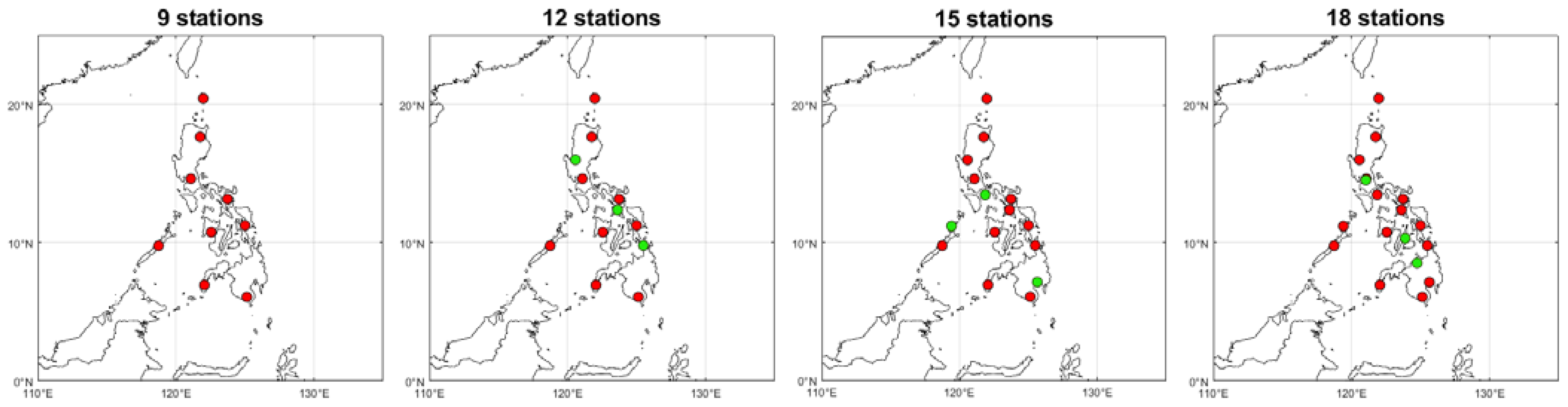
2.1. GNSS Receiver Stations and Receiver Data

The PAGeNet GNSS network currently has 52 active stations running throughout the country [27]. The network can measure any GNSS satellite within range every second. For this study, data from 17 GNSS receiver stations operated by PAGeNet and one IGS station in the Philippines were used. The IGS-operated station is PIMO, while the rest are operated by PAGeNet. The locations of these stations are shown in Figure 1. Currently, there are only about 4 IGS receiver stations stationed in the Philippines. Comparing this to the 52 active stations by PAGeNet, this network can cover more ground in observing the ionosphere than the coverage of the IGS stations.

These stations receive satellite data and store them as receiver independent exchange (RINEX) files. The format was developed to store necessary observables to store GNSS data. The file format has numerous versions and comes in a daily or hourly data. For this study, version 2.11 and the daily file was used [28]. The RINEX files recorded for March 2015 were used in the study.

GIMs, using data from the IGS network, are processed and produced by institutions called analysis centers and are saved as an ionosphere map exchange (IONEX) file. While the IGS has many analysis centers for processing GIMs, the GIM that was used for this study was the one processed by Center for Orbit Determination in Europe (CODE). As mentioned, the spatial resolution of GIMs is 2.5° × 5.0°. Linear bivariate interpolation is used to map vertical TEC within the resolution [29].

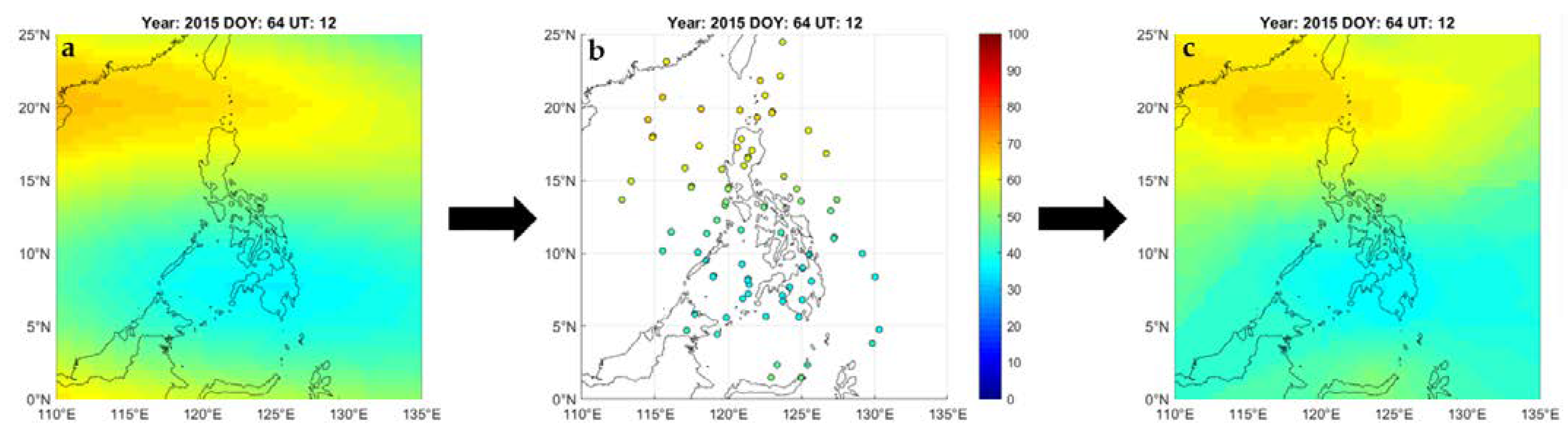
2.2. Developing Regional TEC Maps Using Kriging Interpolation

The chosen parameter used to express electron density for this study is the total electron content. The TEC is defined as the line integral of the electron density $N_e$ along a straight path $l$ between the satellite and receiver. This is expressed in the following equation:

$$TEC=\int N_{e}dl$$

(2)

When the path $l$ is directly perpendicular to the surface of Earth, this is known as the vertical TEC (VTEC). Any other path that is not perpendicular to the surface is known as the slant TEC (STEC). TEC is measured in total electron content units (TECU), equivalent to 10¹⁶ electrons per square meter. For kriging, the mapping involves the use of TEC and its location of observation.

The ionosphere is assumed to be a thin-spherical shell with an altitude $h$ [30]. This study assumed $h$ to be 450 km. The point at which this shell intersects with the line between a given satellite and a receiver in-range is known as the ionospheric pierce point (IPP). This is the spatial element needed for kriging. The electron density along the line of sight at the IPP is STEC. Rotating this line along the radius of Earth, the electron density at the IPP is the VTEC.

Given the satellite elevation $El$ and azimuth angles $A$, the IPP, expressed in geographic coordinates $\left({\phi }_{pp},{\lambda }_{pp}\right)$, was expressed as:

$${\phi }_{pp}={\sin }^{-1}\left[\sin {\phi }_u\cos {\Psi }_{pp}+\cos {\phi }_u\sin {\Psi }_{pp}\cos A\right]$$

(3)

$${\lambda }_{pp}={\lambda }_u+{\sin }^{-1}\left(\frac{\sin {\Psi }_{pp}\sin A}{\cos {\phi }_{pp}}\right)$$

(4)

where $\left({\phi }_u,{\lambda }_u\right)$ are the geographic coordinates of the receiver station in latitude and longitude, ${\Psi }_{pp}$ is the angle between the receiver station and the IPP from the center of Earth. Assuming that the radius of Earth $R_e$ is 6371 km, this angle was calculated as [31]:

$${\Psi }_{pp}=\frac{\pi }{2}-El-{\sin }^{-1}\left(\frac{R_e}{R_e+h}\cos El\right)$$

(5)

By this point, the slant TEC can be calculated based on phase and group delays of dual-frequency satellite transmissions [5,6]:

$$STEC=\frac{1}{40.3}\frac{f_1^2{f}_2^2}{f_1^2-f_2^2}\left[{\rho }_2-{\rho }_1+c\left(DC{B}_r+DC{B}_s\right)\right]$$

(6)

where ${\rho }_1$ and ${\rho }_2$ are the pseudoranges of the satellite frequencies $f_1$ and $f_2$, respectively. The pseudoranges were taken from the RINEX files of the chosen receiver stations. $DC{B}_r$ and $DC{B}_s$ are the receiver and satellite differential code biases (DCB_s), and $c$ is the speed of light.

DCB calculation was completed using the M_DCB MATLAB code developed by Jin et al. [20]. The code prompts for the order of spherical harmonics to be used. This study used four as the authors recommended. Another error in the GNSS measurement is the multipath error. This is when radio signals reach the receiver antennae by two or more paths. This is usually caused by signals reflecting off ground obstacles, such as mountains and buildings [32]. To limit multipath effects, an elevation mask was applied by excluding satellites whose signals were observed at angle of the elevation mask and below. The elevation mask for this study was 25°.

To convert slant TEC to vertical TEC, a zenith-dependent mapping function was ap-plied to the STEC, known as the obliquity factor. This is expressed as [33]:

$$VTEC=STEC\cos \left[{\sin }^{-1}\left(\frac{R_e\sin \chi }{R_e+h}\right)\right]$$

(7)

where $\chi$ is the zenith angle. The zenith angle is the angle between the vertical line at the IPP and the line of sight of the satellite. This is also complementary to the elevation angle of the satellite. At this point, the spatial dataset is complete. This dataset is used as the input for kriging interpolation.

The assumption in ordinary kriging is that, for any position in space $x$ in its neighborhood, the spatial data are stationary [23]. This is mathematically expressed in the following equations:

$$\begin{gathered} E\left[Z\left(x\right)\right]=m \\ E\left[Z\left(x+d\right)-Z\left(x\right)\right]=0 \end{gathered}$$

(8)

$$var\left[Z\left(x+d\right)-Z\left(x\right)\right]=E\left\{{\left[Z\left(x+d\right)-Z\left(x\right)\right]}^2\right\}=2\gamma \left(d\right)$$

(9)

Equation (8) tells us that the expectation value of the spatial function $Z\left(x\right)$ is constant and does not depend on the position $x$. Equation (9) expresses the variance between two points and only depends on the distance between measurements $d$. $\gamma \left(d\right)$ is the semivariogram as a function of the distance between two measurement positions $d$. This expresses the semivariance, which is the spatial relationship of the data.

For a geographic area with multiple stations, a spatial dataset of VTEC for that area can be recorded at any given time. From this dataset, a VTEC map can be produced by redistributing that dataset into a grid of equally spaced points. Each point of the grid would have a corresponding VTEC value. This is similar to the nature of GIMs. The next step was then to determine the VTEC value in each of these grid points.

The VTEC at each grid point was estimated using the 5 geographically closest observed VTEC values in the dataset as [34]:

$$\widehat{Z}\left(x_0\right)={\displaystyle \sum }_{i=1}^n{\lambda }_{i}Z\left(x_i\right)$$

(10)

where $\widehat{Z}$ is the estimated VTEC at the grid point $x_0$, $Z$ is the VTEC observed at location $x_i$, ${\lambda }_i$ is the weight value. As 5 closest points were used, $n$ was set to 5. Thus, $\left\{Z\left(x_1\right),Z\left(x_2\right),\dots ,Z\left(x_5\right)\right\}$ are VTEC values that are closest to $Z\left(x_0\right)$. Based on Equation (9), the weights ${\lambda }_i$ were calculated using the following matrix equation [22,23]:

$$\left[\begin{array}{c}{\lambda }_1\\ ⋮\\ {\lambda }_n\\ \mu \end{array}\right]=\left[\begin{array}{c}\gamma \left(x_1,x_0\right)\\ ⋮\\ \gamma \left(x_n,x_0\right)\\ 1\end{array}\right]{\left[\begin{array}{cccc}\gamma \left(x_1,x_1\right)& \cdots & \gamma \left(x_1,x_n\right)& 1\\ ⋮& \ddots & ⋮& ⋮\\ \gamma \left(x_n,x_n\right)& \dots & \gamma \left(x_n,x_n\right)& 1\\ 1& \cdots & 1& 0\end{array}\right]}^{-1}$$

(11)

where $\gamma \left(x_i,x_j\right)$ is the semivariogram at a distance between points $x_i$ and $x_j$. To determine the semivariogram, an experimental semivariogram was constructed first from the observed dataset by using the following [34]:

$$\widehat{\gamma }\left(h_j\right)=\frac{1}{2m\left(d_j\right)}{\displaystyle \sum }_{i=1}^{m\left(h_j\right)}{\left[Z\left(x_i\right)-Z\left(x_j\right)\right]}^2$$

(12)

The function $m\left(d_j\right)$ represents the number of pairs of measurement $Z\left(x_i\right)$ separated by distance $d$ within the interval $\left[d_j,d_{j+1}\right]$ [23]. A theoretical variogram was then developed by fitting a model to the experimental semivariogram [22,24,34]. The process was repeated for every point in the grid. An example of the experimental and theoretical variogram is shown in Figure 2.

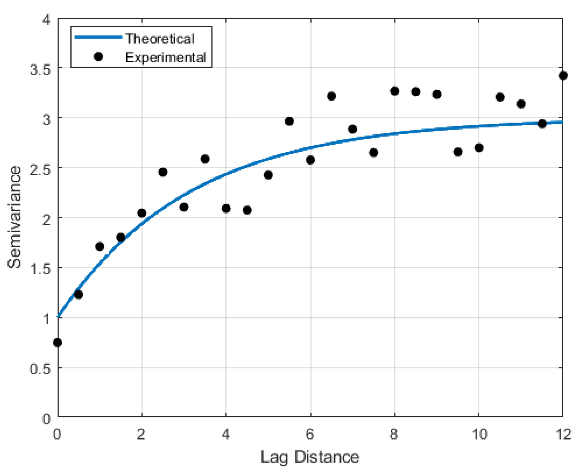
2.3. Finding the Optimum Parameters for Kriging Interpolation

Varying the number of receiver stations used will also vary the size of the spatial dataset. A smaller spatial dataset may underrepresent the map. On the other hand, a larger spatial dataset will make calculations take longer. There are also multiple semivariogram models used to fit the experimental variogram. Other studies would assume the model. However, a variogram that best describes the spatial relationship of the spatial dataset of the VTEC in the Philippines would be very preferrable. This step tries to find out which is the best number of samples to be used as well as the best-fitting semivariogram model as the optimum set of parameters by using an established map, GIM, and reconstruct it using kriging. The original and the reconstructions were then compared.

Instead of arbitrarily choosing points in the GIMs, actual GNSS positional data from the selected stations were used and determined the GIM VTEC at those points. By changing the number of stations for mapping, the sample size of the dataset is changed. This study used 9, 12, 15 and 18 stations in the Philippines. The selection and distribution of the stations is illustrated in Figure 3. At any given time, each GNSS station can observe at least 6 GPS satellites.

As for the optimum variogram model, many functions can be used to model variograms. However, the three most used are linear [34]:

$$\gamma \left(d\right)=c_0+bd$$

(13)

spherical:

$$\gamma \left(d\right)=\left\{\begin{array}{c}{c}_0+c\left[\frac{3}{2}\frac{d}{r}-\frac{1}{2}{\left(\frac{d}{r}\right)}^3\right], 0\le d\le r\\ c_0+c, d>r\end{array}\right.$$

(14)

and exponential:

$$\gamma \left(d\right)=c_0+c\left[1-\exp \left(-\frac{3d}{r}\right)\right]$$

(15)

For each equation, there are unknown coefficients that need to be determined. In the linear model, these coefficients are $c_0$ and the slope $b$. The spherical and exponential methods have the same unknown coefficients $c_0$, $c$ and $r$. $r$ is called the effective range. This denotes the furthest extent of the variogram correlation. Any two points that are at a distance greater than $r$ have zero correlation. These models were fitted to the experimental semivariogram. Using non-linear least squares estimation, the unknown coefficients were determined based on how well they fit into the experimental semivariogram. To test which set of parameters was optimum, IGS GIMs were reconstructed by using the kriging method. IGS VTEC data were used as TEC data input, whereas observed satellite IPP data were used for spatial input.

Using the positional data, the GIM VTEC value at the specific set of IPP data was extracted from IGS GIMs. This set of TEC and spatial data was then used to reconstruct the same GIM map. Figure 4 illustrates how this process of GIM extraction and reconstruction works. As the number of receiver stations and the semivariogram model vary, 12 different TEC maps were created based on 1 IGS GIM VTEC map.

As the number of GNSS stations and the type of theoretical semivariogram vary as shown in Figure 3 and Equations (13)–(15), respectively, there are 12 possible ways to reconstruct a single IGS GIM. Twelve different mapping scenarios could be created with three different semivariogram models and four sampling sizes. Each of these scenarios was compared with the original GIM. The optimum set would be the scenario that was the closest to the original GIM. This was measured using the normalized error. The normalized error closest to zero meant that there was not much difference between it and the original map. The normalized error is defined as [35]:

$${ϵ}_n=\frac{{{\displaystyle \sum }}_{i=1}^N{\left[\widehat{Z}\left(i\right)-Z\left(i\right)\right]}^2}{{{\displaystyle \sum }}_{i=1}^N{\left[Z\left(i\right)\right]}^2}$$

(16)

where $Z\left(i\right)$ is the TEC of the GIM map at the $i$th grid point, and $\widehat{Z}\left(i\right)$ is the TEC of the kriging map at the $i$th grid point.

The GIMs reconstructed were taken from 12 dates within March 2015. These dates were 1–3, 5, 6, 17, 18, 25–28, 30 March. The availability of data for all sets of receivers and the space weather and geomagnetic conditions were considered in choosing the dates. 1, 2, 17 and 18 March were geomagnetically active days. 25, 27, 28 and 30 March were geomagnetically quiet days. 3, 5, 6 and 26 March have scintillations events that occurred. Thus, each ionospheric condition equally has 4 dates for this step. The time resolution of GIMs used in this study is 2 h. From this alone, 96 GIMs were taken, and, with the different parameter sets, 1152 maps were recreated using kriging.

In summary, to find out which parameter set is optimum, the kriging method is used to recreate GIMs. First, a GIM was extracted from the IONEX file. Four sets of receiver stations were used based on Figure 3 that vary in size, and their positional data would be used to extract GIM VTEC. With the four sets of receivers, this means that there are four ways to extract the VTEC in the GIM map in which the number of points varies. This set of GIM VTEC and GNSS locations would be reconstructed using kriging. Before reconstruction, an experimental semivariogram was produced based on the spatial dataset and then fitted into a theoretical variogram. As there are 3 semivariogram models considered for this study, each spatial dataset would produce three different maps based on the model of the theoretical variogram. With 4 sets of receiver stations and 3 types of semivariogram models, 12 maps can be produced based on a single IGS map. GIM maps from the chosen dates of March 2015 were taken and reconstructed. The chosen dates have their ionospheric and geomagnetic conditions considered. A total of 1,152 maps were reconstructed from 96 GIMs.

2.4. Analysis of TEC Maps

With the use of the optimum parameters, the mapping method was applied to the actual GNSS TEC data over the Philippines during different space weather conditions, and the results were analyzed. The spatial resolution of these maps was 0.5° × 0.5° in latitude and longitude. The temporal resolution was 1 h. TEC maps only showed the spatial trend of the ionosphere. A time series of maps was developed using data recorded every two hours, totaling 12 maps in an observation day. The range of the map is 110° to 135° in longitude and 0° to 25 in latitude. This area corresponds to the Philippine region and parts of its surrounding countries. Contour plots that show the spatiotemporal variation in the maps in terms of latitude and longitude were also produced. This was completed by creating a VTEC map with a time resolution of 1 h. The average VTEC was taken across all longitudes within each latitude. The average VTEC was taken across all longitudes within each latitude and vice versa.

3. Results

3.1. Optimum Parameters for Kriging

Given that the time resolution was 2 h, each chosen day has 12 maps. Thus, each day has 12 normalized error values. These error values were averaged to produce the mean normalized error of that day for a single parameter set. With a mean value, this also comes with a standard deviation value. This shows that the normalized error varies much throughout the day. The mean normalized error values and their corresponding standard deviation values are shown in

Table 1. Mean normalized error (MNE) values throughout 12 days of March 2015. Values in bold and in green indicate the best-performing parameter set on that day. The worst-performing sets are in red.

No. of Stations	Model	DOY 60	DOY 61	DOY 62	DOY 64	DOY 65	DOY 76
9	linear	0.00442	0.00437	0.00436	0.00450	0.00567	0.00435
	spherical	0.00475	0.00471	0.00468	0.00488	0.00584	0.00460
	exponential	0.00554	0.00560	0.00566	0.00582	0.00676	0.00545
12	linear	0.00414	0.00425	0.00431	0.00443	0.00546	0.00432
	spherical	0.00434	0.00451	0.00457	0.00472	0.00562	0.00454
	exponential	0.00498	0.00524	0.00539	0.00554	0.00640	0.00528
15	linear	0.00402	0.00417	0.00420	0.00438	0.00569	0.00414
	spherical	0.00418	0.00436	0.00440	0.00460	0.00582	0.00434
	exponential	0.00472	0.00498	0.00508	0.00528	0.00647	0.00499
18	linear	0.00403	0.00418	0.00421	0.00440	0.00566	0.00415
	spherical	0.00418	0.00435	0.00438	0.00461	0.00579	0.00433
	exponential	0.00468	0.00493	0.00502	0.00525	0.00644	0.00493
No. of Stations	Model	DOY 77	DOY 84	DOY 85	DOY 86	DOY 87	DOY 89
9	linear	0.00492	0.00360	0.00320	0.00391	0.00332	0.00300
	spherical	0.00539	0.00387	0.00342	0.00418	0.00357	0.00324
	exponential	0.00672	0.00438	0.00406	0.00486	0.00428	0.00381
12	linear	0.00516	0.00352	0.00314	0.00387	0.00331	0.00301
	spherical	0.00557	0.00377	0.00333	0.00410	0.00351	0.00320
	exponential	0.00678	0.00424	0.00391	0.00472	0.00419	0.00371
15	linear	0.00531	0.00347	0.00315	0.00399	0.00336	0.00304
	spherical	0.00565	0.00363	0.00332	0.00416	0.00353	0.00319
	exponential	0.00671	0.00407	0.00383	0.00469	0.00413	0.00361
18	linear	0.00539	0.00343	0.00315	0.00398	0.00336	0.00305
	spherical	0.00571	0.00359	0.00331	0.00414	0.00352	0.00319
	exponential	0.00671	0.00401	0.00380	0.00466	0.00410	0.00358

and

Table 2. Standard deviation values of the mean normalized error throughout 12 days of March 2015. Values in bold and in green indicate the least value on that day. The worst-performing sets are in red.

No. of Stations	Model	DOY 60	DOY 61	DOY 62	DOY 64	DOY 65	DOY 76
9	linear	0.00502	0.00436	0.00531	0.00469	0.00338	0.00252
	spherical	0.00527	0.00455	0.00551	0.00495	0.00346	0.00272
	exponential	0.00593	0.00528	0.00627	0.00561	0.00412	0.00343
12	linear	0.00495	0.00418	0.00529	0.00466	0.00326	0.00250
	spherical	0.00506	0.00429	0.00542	0.00484	0.00332	0.00265
	exponential	0.00550	0.00479	0.00592	0.00531	0.00374	0.00318
15	linear	0.00507	0.00421	0.00538	0.00476	0.00349	0.00246
	spherical	0.00513	0.00428	0.00546	0.00487	0.00353	0.00259
	exponential	0.00539	0.00460	0.00580	0.00523	0.00386	0.00297
18	linear	0.00501	0.00418	0.00532	0.00473	0.00341	0.00238
	spherical	0.00506	0.00423	0.00538	0.00483	0.00348	0.00247
	exponential	0.00532	0.00452	0.00569	0.00516	0.00385	0.00280
No. of Stations	Model	DOY 77	DOY 84	DOY 85	DOY 86	DOY 87	DOY 89
9	linear	0.00330	0.00206	0.00285	0.00232	0.00231	0.00357
	spherical	0.00359	0.00220	0.00308	0.00243	0.00256	0.00380
	exponential	0.00450	0.00225	0.00371	0.00275	0.00300	0.00433
12	linear	0.00321	0.00203	0.00285	0.00231	0.00232	0.00354
	spherical	0.00347	0.00216	0.00304	0.00240	0.00249	0.00372
	exponential	0.00428	0.00223	0.00360	0.00271	0.00295	0.00416
15	linear	0.00337	0.00203	0.00281	0.00244	0.00235	0.00354
	spherical	0.00358	0.00209	0.00300	0.00251	0.00251	0.00368
	exponential	0.00428	0.00221	0.00351	0.00280	0.00296	0.00405
18	linear	0.00340	0.00201	0.00279	0.00242	0.00233	0.00357
	spherical	0.00361	0.00208	0.00297	0.00250	0.00249	0.00370
	exponential	0.00427	0.00220	0.00345	0.00279	0.00294	0.00403

.

As shown in Table 1 and Table 2, the mean errors and standard deviations are very minimal across all parameter sets. Thus, any of these sets could work in mapping the Philippines. In terms of mean, two sets performed the best, 12 stations with the linear model and 15 stations with the linear model. Both sets performed the best in 5 out of 12 days. Further, nine stations with the linear model and eighteen stations with the linear model performed the best on one day each. In terms of the standard deviation, 12 stations with the linear model performed the best in 7 out of 12 days. For 3 days, the parameter 18 stations with the linear model was the best-performing set. For 2 days, nine stations with the linear model and 15 stations with the linear model each performed the best on one day. From these results, all best-performing parameter sets have their models in the linear model. As for the number of stations, 12 stations and 15 stations were the candidates for the optimum number of stations. A bar graph was constructed to visualize how each number of stations performed in each day along with the linear model shown in Figure 5.

This shows that twelve stations performed the best on most days, with eleven instances being the best-performing parameter in terms of mean and standard deviation, followed by fifteen stations, then eighteen and, last, nine stations. This means that the optimum set of parameters is 12 stations, and the linear model has frequently shown the least error on average, which does not deviate as much throughout the day. The maps in the next section made use of this parameter set.

The reasons as to why these exact parameters performed the best is unknown. However, it is noted that interpolation used in GIMs is also linear. Some studies compared multiple models, fitted them to their data from other geographic areas and yielded different results [24,36]. However, their methods of determining the best fit model differed from the method of this study. As for 12 stations, this may have to do with the sampling size or distribution. There comes a point in kriging where adding more samples does not improve the performance of the mapping [35]. The pattern that the samples took in 12 stations may have played a role in its results even just a little since 15 stations performed just as well as 12 stations in terms of the mean normalized error.

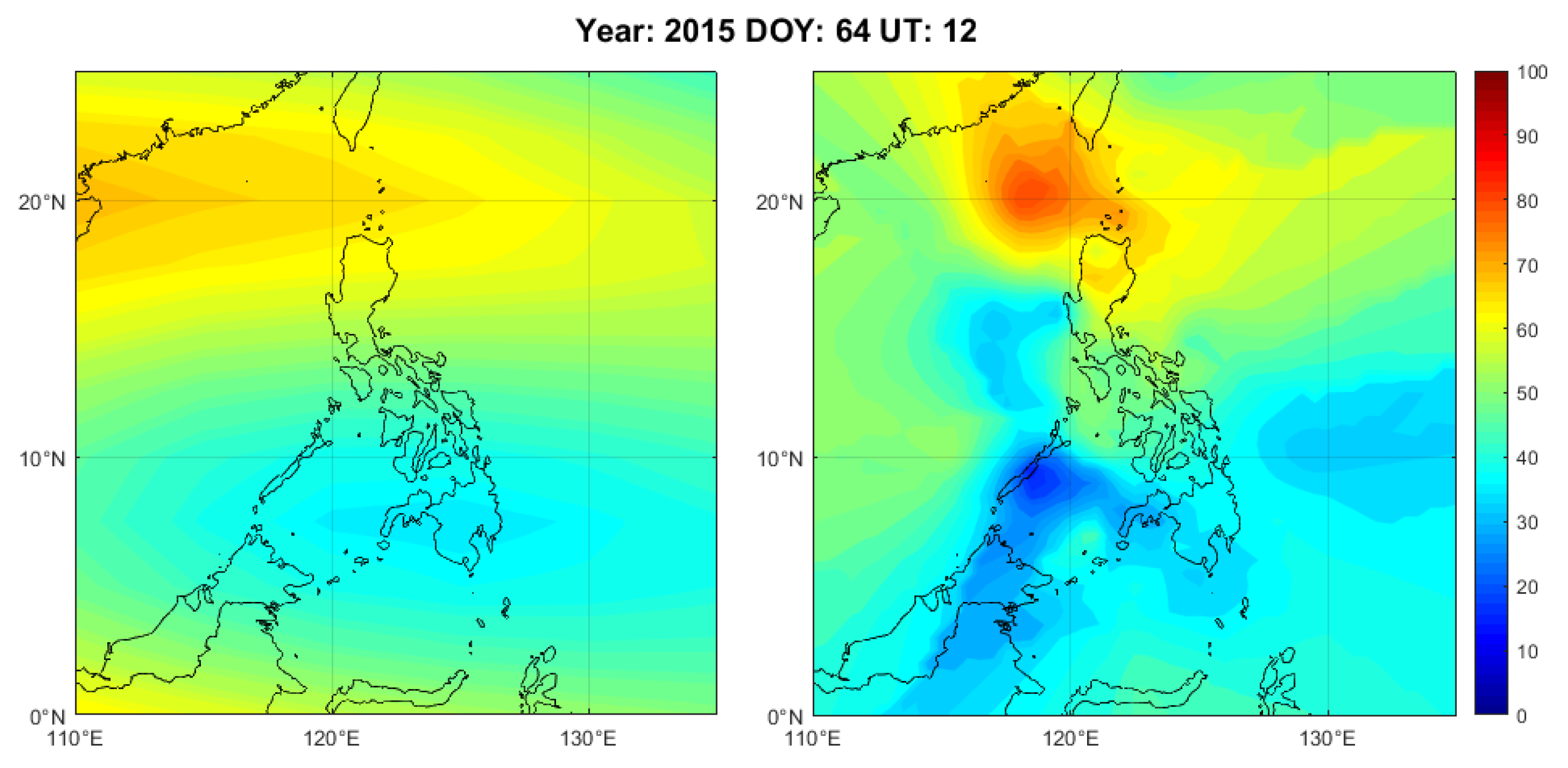
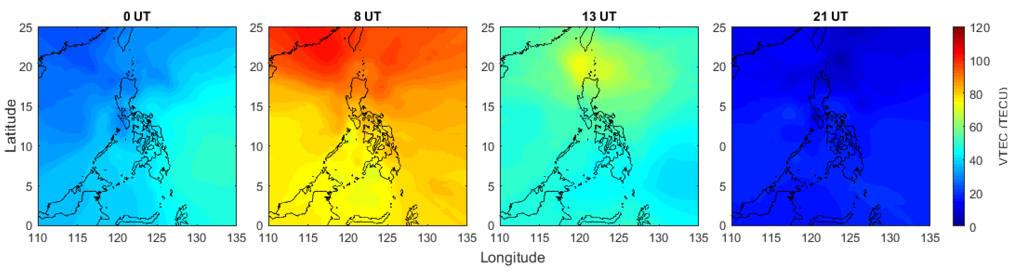
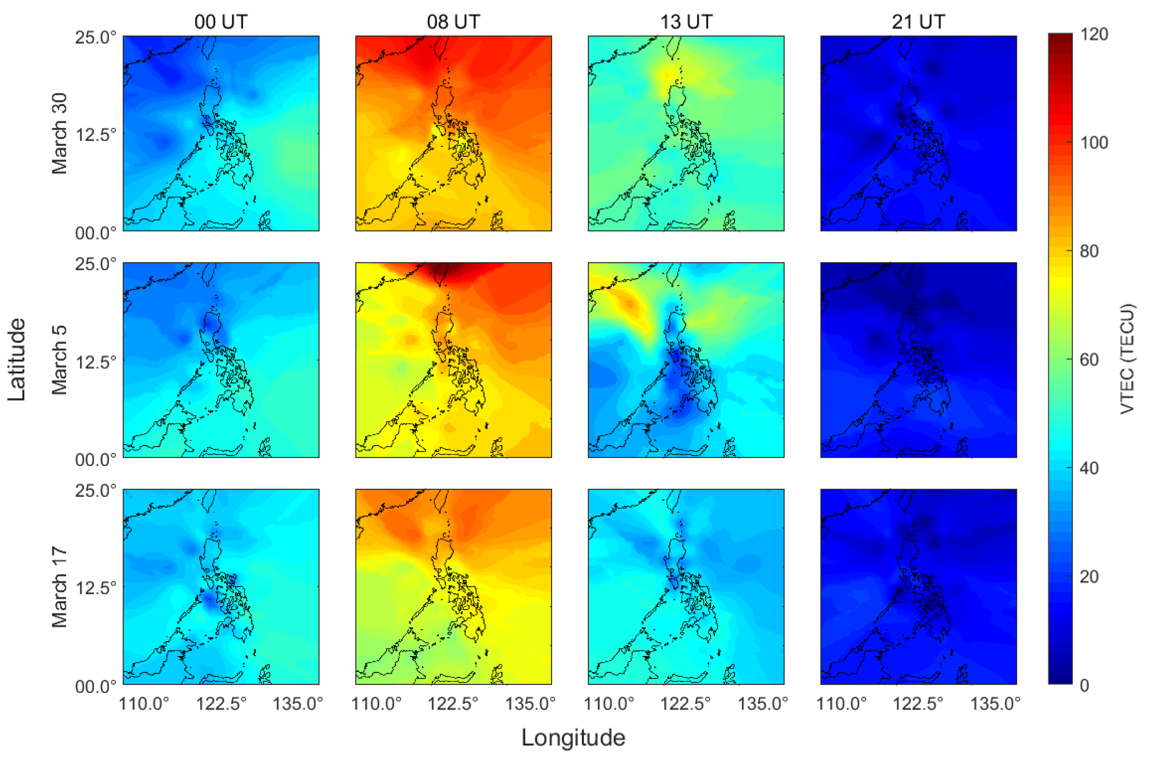
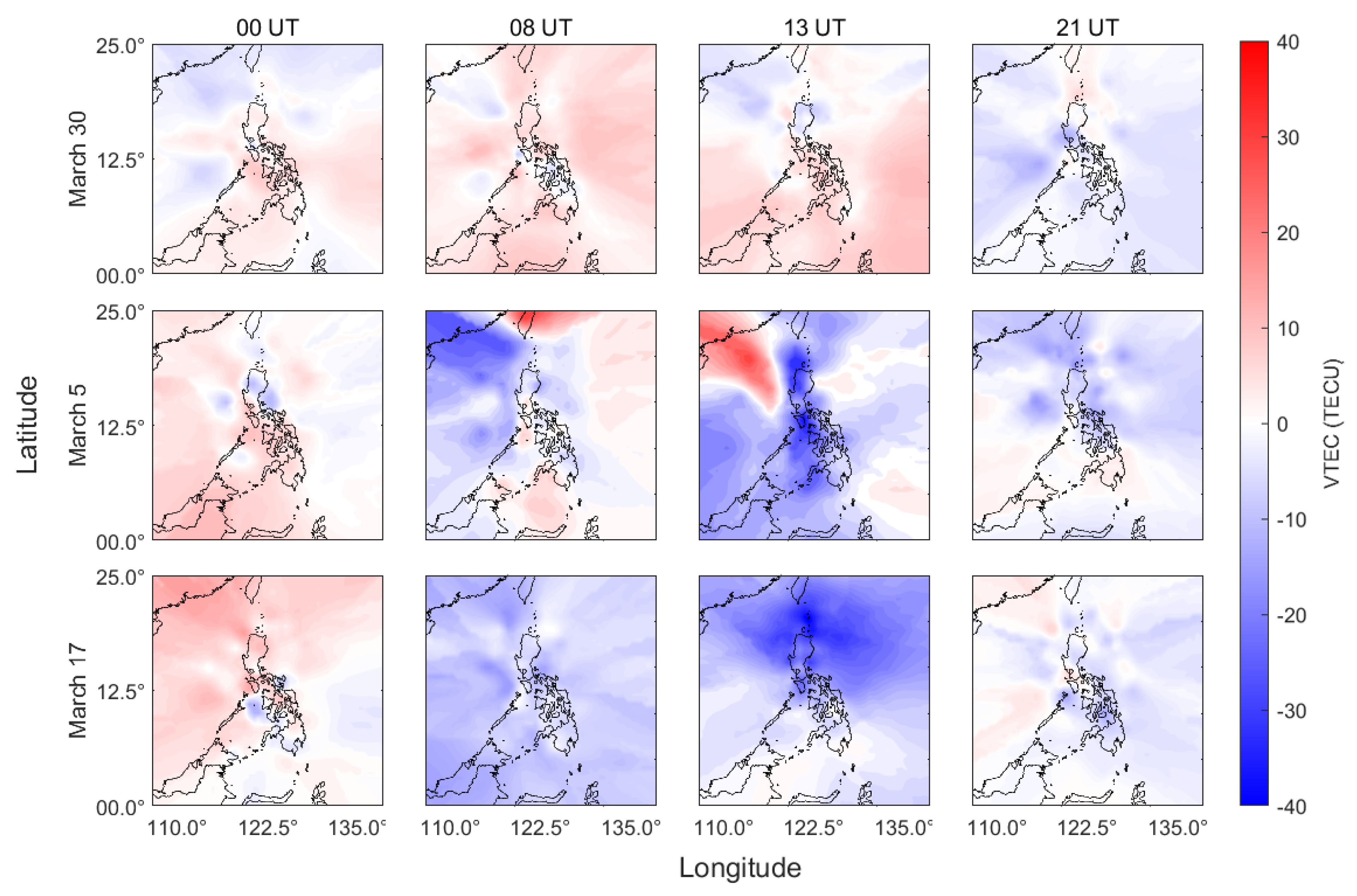
3.2. GNSS VTEC Maps over the Philippines

As shown in Figure 6, there are obvious differences between the two. VTEC in GIM is depicted to have around 60 TECU around the north side, which steadily increases towards 70 TECU westward. The southern portion is around 30 to 40 TECU and smoothly contrasts the northern side. The map produced by kriging, on the other hand, shows an area of even higher VTEC, reaching about 80 TECU. The southern portion contains a pocket of even lower VTEC, with a VTEC of around 20 TECU. This goes to show how under-sampled GIMs are as the kriging maps were produced with a higher sampling rate compared to GIMs. Next is to see how the kriging maps perform under different geomagnetic conditions.

First, a one-dimensional VTEC profile was produced to show the behavior and variability in VTEC during quiet, active and scintillated geomagnetic events. A single date was chosen to represent the behavior of VTEC during that specific geomagnetic condition. The dates 30 March, 17 March and 5 March were chosen to represent a quiet day, an active day and a scintillated day, respectively. Additionally, March 2015 has 11 dates that were geomagnetically quiet. These dates were averaged to create an average quiet day VTEC profile. This should show general behavior of the ionosphere throughout the day when undisturbed for the observed month. This shows how VTEC varies and contrasts during different ionospheric conditions. Figure 7a illustrates the one-dimensional VTEC during the chosen dates and the average quiet day VTEC. Figure 7b shows the differences between the chosen dates and the average quiet VTEC. Moreover, Figure 8 shows the geomagnetic and space weather conditions on those same days in terms of the planetary K-index and the F10.7 solar index.

On an average quiet day, the VTEC started at around 30 TECU at 0 UT, then peaked before 8 UT. It started to decrease as it approached 12 UT. An enhancement in VTEC was observed during these times, peaking at around 13:30 UT with a VTEC of 60 TECU. After this peak, the VTEC decreased to a minimum at around 21 UT. The stormy day started just a bit higher, with VTEC almost reaching 40 TECU, then maximized at around 75 TECU, which is lower than average. The K-index increased from 2 to 5 starting at 3 UT, denoting a geomagnetic storm. A sharp decrease was observed at around 12 UT, making VTEC much lower than average. The K-index would be at its highest starting from this time as well. During minimum, active day VTEC increased slightly, closely matching to the average quiet VTEC. Further, 30 March was slightly higher during times of high VTEC and started to decrease towards a minimum earlier than average. Its minimum was slightly lower than the average minimum. The planetary K-indices during this day indicated that this day was geomagnetically quiet. On 5 March, the VTEC started normally. However, its maximum was lower than the average quiet day VTEC. An irregular dip was observed at 13 UT before quickly increasing and decreasing towards the minimum. The minimum VTEC during this day was much lower than the average quiet VTEC. The K-indices also indicated that this day was geomagnetically quiet. The solar flux on these days show that 5 March and 30 March have a similar solar flux, which lines up with their similarity in K-indices. The solar flux on 5 March was significantly lower than the other two dates while having higher K-indices.

The differences across all three dates did not exceed ±30 TECU. The differences between 30 March and the average were consistent and did not exceed ±10 TECU. During the first part of 30 March, VTEC was higher than average, while, during the latter part, it was lower. On 5 March, VTEC was lower than average for most of the day. The noisy dip was once again observed after 12 UT. VTEC was higher than average on 16 UT. On 17 March, the VTEC started higher then decreased into negative values and started higher again by 8 UT. At 12 UT, a sharp increase in difference occurred, which became higher than average. Then, it went back to the negatives. The difference slowly increased again. By around 22 UT, the VTEC differences went back to positives. Compared to quiet days, active and scintillated days significantly differed to them at around 13 UT as the differences exceeded more than 10 TECU.

All three conditions started similarly but then differed after the 12 UT mark. The average quiet day is characterized by enhancements in VTEC after said time. This is characteristic of the nighttime TEC enhancement. The exact causes of these enhancements are still being investigated; however, there is a connection between them and the reverse fountain effect after sunset [37]. This suggests that the reverse fountain effect on 30 March is not as intense as the one on average. The irregularity found on 5 March is characteristic of ionospheric scintillations.

The storm that occurred on 17 March, also known as the St. Patrick’s Day storm, was a negative storm due to the observed depletion in VTEC. The depletion on this date could be caused by perturbations of neutral gases in the ionosphere. The density of neutral O₂ and N₂ increases while atomic oxygen density decreases. This causes the ionosphere to be composed of more neutrals than ions, hence a depletion of TEC [21]. It has also been confirmed that O/N₂ decreased in Asian sectors the day after the storm [38]. This storm was caused by a coronal mass ejection (CME) from the Sun that occurred on March 15. It reached Earth on St. Patrick’s Day, 17 March, creating the strongest geomagnetic storm of Solar Cycle 24 [38,39].

This method of studying the VTEC around the Philippines is exactly the method that Mendoza [21] used. A constraint is that only VTEC at specific points can be observed. Although the latitudinal distribution was considered, the longitude was not. He also mentioned how the GIM-based method for calculating VTEC introduces potential errors due to the lower spatial resolution of GIMs. The transition from one dimension to two dimensions may just provide more context surrounding the VTEC in the region.

The spatial resolution and range of the maps produced and shown in Figure 9, Figure 10 and Figure 11 are the same as the ones in the previous section. The maps were during the same dates and at times 0, 8, 13 and 21 UT, which correspond to 8 am, 4 pm, 9 pm and 5 am in local time and are the two-dimensional versions of Figure 7. These times were chosen based on Figure 7, where 8 and 21 UT represent the maximum and minimum VTEC of the day, respectively, and 13 UT represents the point where VTEC deviates the most from the average across all space weather events. Further, 0 UT marks the start of the day and serves as a neutral point in time as there was not much difference observed in Figure 7.

First, two-dimensional maps were produced for the average quiet day VTEC at the selected times illustrated in Figure 9. On an average quiet day, the VTEC starts higher around the eastern region than in the west, with VTEC almost reaching 60 TECU at 0 UT. At 8 UT, a north–south VTEC gradient was observed. The southern side had a VTEC of around 70 TECU, while the north had around 80–90 TECU. At 13 UT, the gradient was still maintained, albeit lower than what was observed at 8 UT. The VTEC level at 21 UT was generally below 10 TECU. What is shown in the 2d maps lines up mostly with Figure 7, considering it is only a 1d map.

Figure 10 illustrates the TEC maps during the same select days as Figure 7. In this figure, the measurements at the edges of the map tend to show a more radial pattern extending outwards. This is because of the lack of data observed around these areas. The 0 UT maps across all three days appeared to be very similar, which agrees with the one-dimensional profile observations. As this was still in the morning, the eastern portion of the map was higher than the west as it receives sunlight first, thus more ionization in the region. During high VTEC at 8 UT, the north–south gradient is observable again, as in Figure 9. The quiet day shows greater VTEC than both days, with VTEC ranging from around 70 TECU in the south and around 90–100 TECU in the north. During high VTEC at 8 UT, the north–south gradient is observable again, as in Figure 9. The quiet day shows greater VTEC than both days, with VTEC ranging from around 70 TECU in the south and around 90–100 TECU in the north. On the other hand, the active day has VTEC levels of around 60 TECU on the south side, and around 80–90 TECU on the north. On 5 March, there is a small area where VTEC is the highest on the north side, with VTEC reaching almost 120 TECU.

Small pockets of lower VTEC with values below 20 TECU, compared to its surroundings, can be observed but are more prominent at 0 UT. Further investigation of these low VTEC pockets has revealed that these observations are almost all from PURD station. A one-dimensional profile of the PURD station was created, and it was found that the VTEC observed was generally lower than the other receiver stations, especially during low VTEC. This is an example of how input data can affect the resulting maps.

Further, 13 UT is where all three days greatly differ. The north–south gradient is preserved on 5 March and 30 but completely absent on 17 March. The TECU levels on 30 March were higher than the other days, with a VTEC of about 60 TECU, and the north side reaching as far as around 80 TECU. The gradient on 5 March is much greater than that of the quiet day. An area of depleted TEC of only around 20 TECU running vertically from north to south is observed on this date. A zone of higher VTEC is present around the northwest, with a peak of around 80 TECU. At 21 UT, all three days appear to be similar again, with low VTEC spots once again observed by PURD. The VTEC during this time is around 10 TECU for all three dates. To show how the maps in this figure deviate from the average day, Figure 9 was subtracted to Figure 10 on each day, creating Figure 11. The blue zones indicate a lower VTEC than average, red higher and white neutral.

In Figure 11, 5 March and 17 start with areas of higher VTEC than average, with fewer zones where VTEC was lower. Further, 30 March was more neutral, with more white areas. The VTEC difference ranges from ±10 TECU, just as in Figure 7b. At 8 UT, the VTEC on 30 March was still mostly above average compared to the other dates. The VTEC goes up by around 10 TECU, which lines up with Figure 7. On 5 March, the very high VTEC on the north side, seen in Figure 10, was highlighted in the difference map. The VTEC difference around this area was around 30 TECU. Further, 17 March was completely below average, with TEC levels around −10 TECU in difference. This corresponds to Figure 7. At 13 UT, there seems to be a higher VTEC than average in the southern area on 30 March. The gradient on 5 March emphasizes that the northwest area is much higher than average, with a VTEC difference of about 25 TECU, while the central region running down south was much lower, with a VTEC difference of around −30 TECU.

On a scintillated day, the presence of these depleted regions could be a sign of equatorial plasma bubbles (EPBs). As previously mentioned, EPBs are ionospheric irregularities that occur during scintillation events. Depletions in TEC characterize these along with elongated patches that run along the Earth’s magnetic field lines [40]. Further, 17 March in the figure shows how much VTEC has depleted as the northern region is much lower than average as the difference here was close to −40 TECU, and 21 UT showed more areas colored in white as the VTEC on all three dates tended to be closer to the average, which corresponds to Figure 7. As in Figure 7b, the significant difference was at 13 UT as the differences exceeded ±10 TECU.

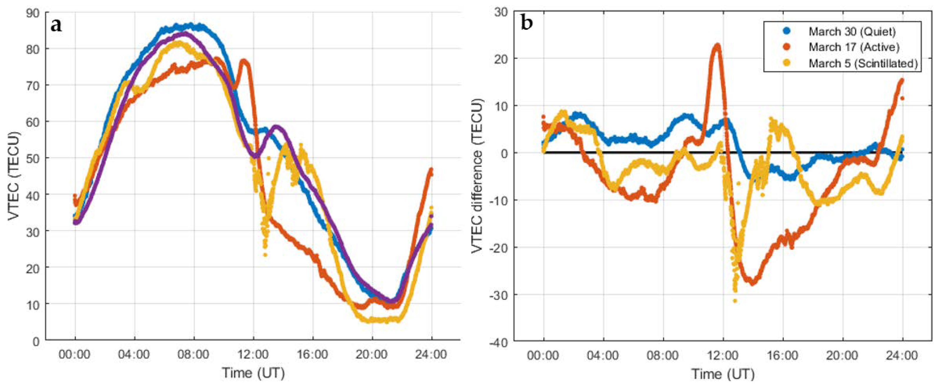
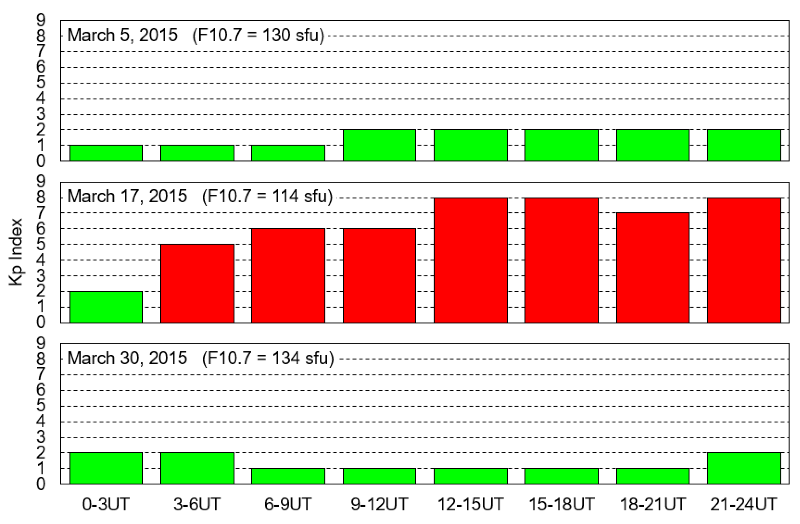
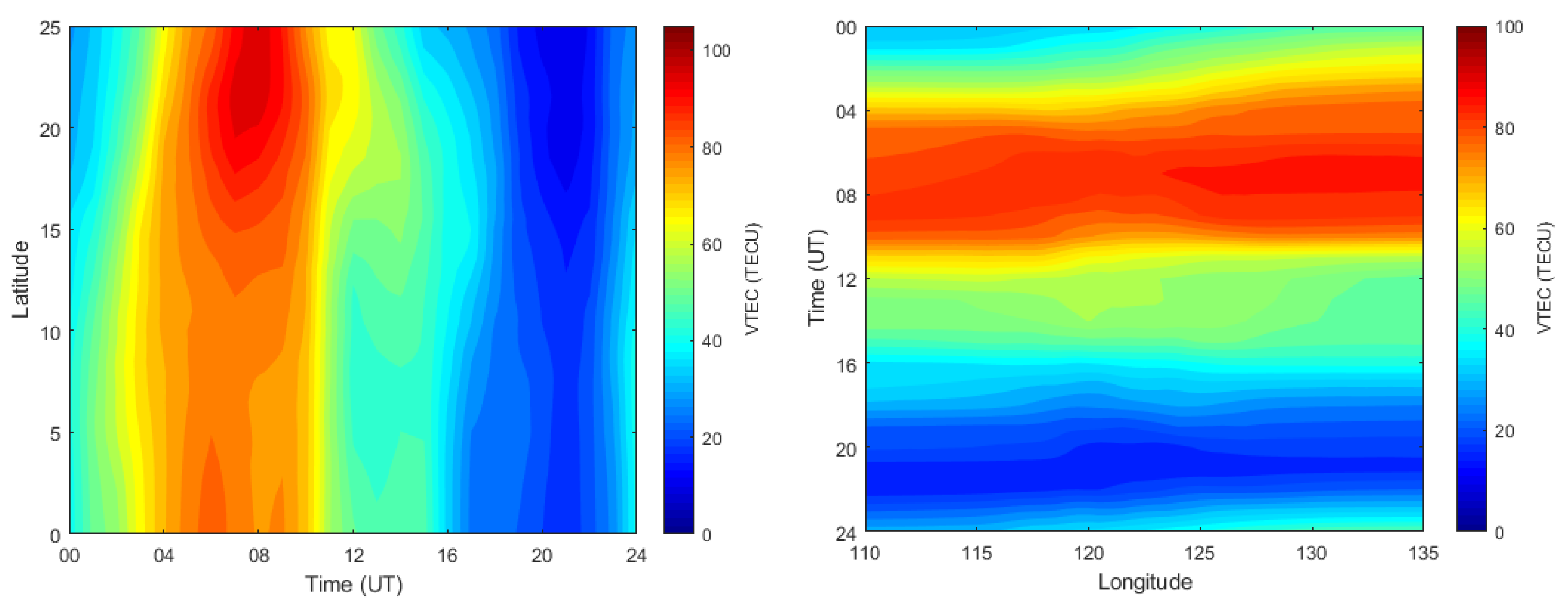
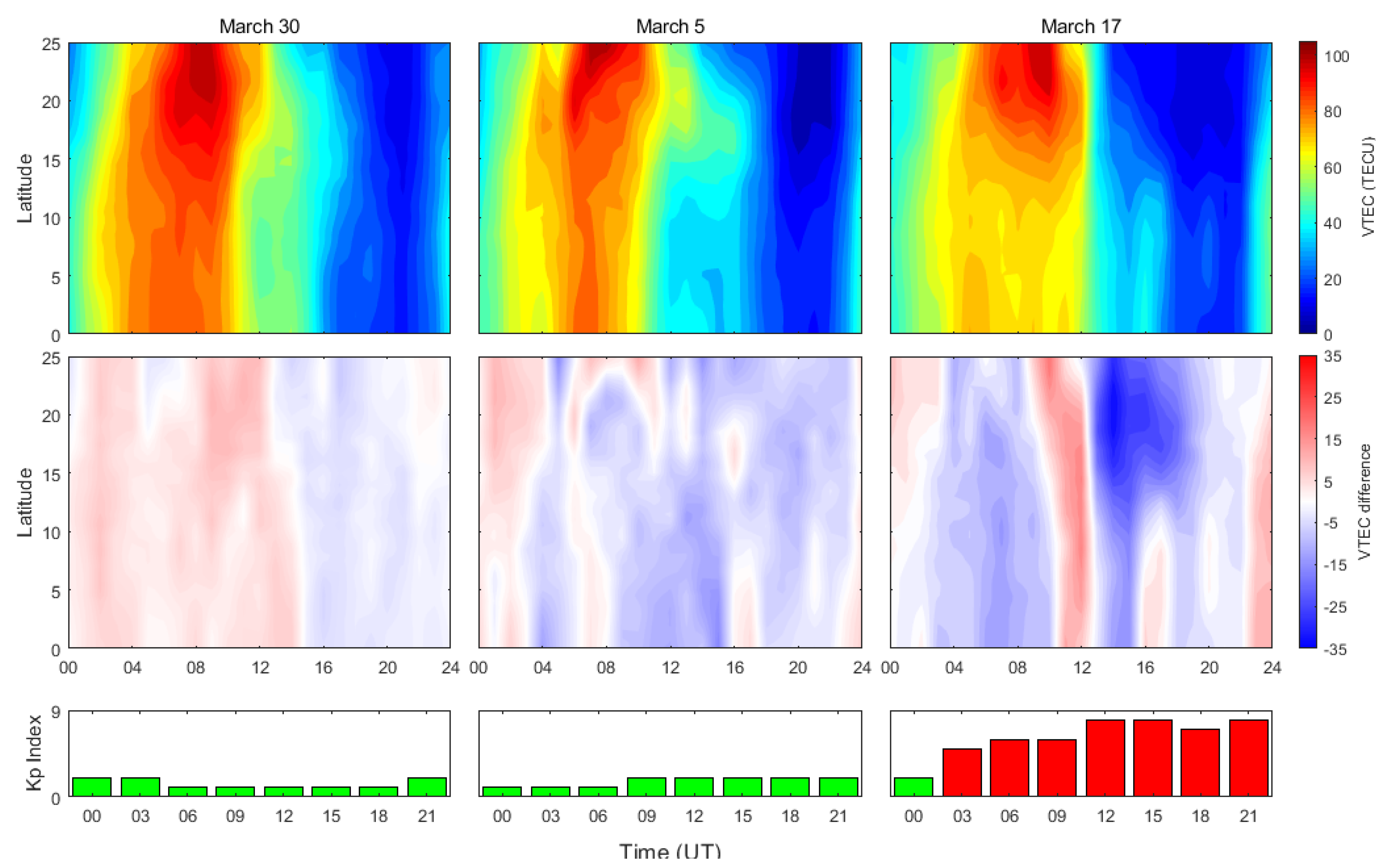
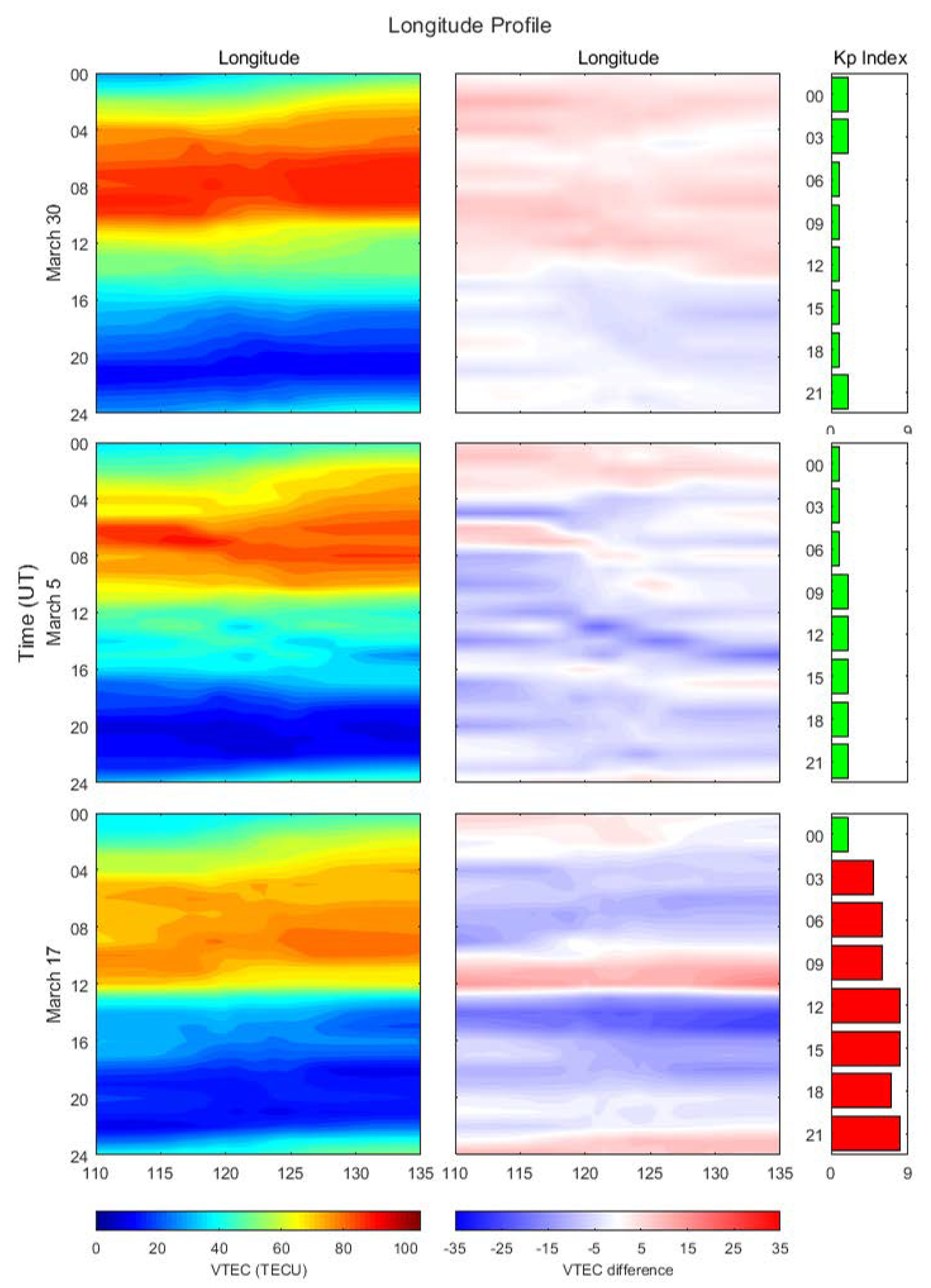
3.3. Spatial and Temporal Analysis

Further spatial analysis of the maps and contour plots called latitude and longitude profiles were generated to check the latitudinal and longitudinal variation. First, a latitude and longitude profile for the average quiet day VTEC was created. The resulting contour plots shown in Figure 12 serve as a reference point for the latitude and longitude profiles for the other days.

A north–south gradient was still present during the day, with the north having a higher VTEC at around 90 TECU and the south having a lower VTEC at around 70–80 TECU. This peaked around 8 UT, which corresponds to Figure 7. Around 12 to 16 UT, the VTEC stayed at around 30–40 TECU. After 16 UT, the VTEC decreased to around 10–20 TECU. There was not much longitudinal variation on an average quiet day. There was only a slight east–west difference observed at the start of the day. At 0 UT, the west was slightly lower, with around 40 TECU, while the east was around 50 TECU. The TEC started to rise by 4 UT, rising to around 80–90 TECU. This lasted up to around 12 UT, when the TEC decreased to around 50 TECU. The VTEC reached a minimum at around 21 UT, where the TEC was around 10 TECU.

Figure 13 shows that the latitudinal gradient was still present on all three days. The Kp-index was included to see how the latitudinal VTEC changes with the geomagnetic activity. This area started to maximize at around 8 UT, corresponding to what was observed in Figure 7. The southern area during 17 March was not as high, with a VTEC level closer to 60 TECU compared to the other dates, which were closer to around 80 TECU. This lines up with Figure 10 at 8 UT, where the VTEC was much lower on the southwest area of the map. The peak VTEC on 5 March did not seem to last as long compared to the other dates. TEC level went to around 70 TECU, except for the extreme north, with around 100 TECU. Further, 30 March seemed to start higher than average and then lower at around 14 UT compared to the average quiet day. This agrees with Figure 7. Further, 5 March had patches of higher and lower values throughout the day and latitudes, although there were more blue areas than red. Considering that the one-dimensional profile was based on observations by PIMO station, this could be a given. On 17 March, the VTEC started low, but it suddenly increased at 12 UT before decreasing again. This lines up with the sharp increase and sudden decrease found in Figure 7. A zone of very low compared to average VTEC can be found in the north after this sharp decline before increasing to close to average at around 18 UT. The Kp-index values also reached their maximum around this time.

Looking at Figure 14, there was not much longitudinal variation on 30 March. Temporally, the VTEC variation was consistent with the latitude profile. The VTEC during the day reached beyond 80 TECU. Its difference was similar to what was observed in the latitude profile, with VTEC going above average during the day and below average during the night. The difference values only ranged around ±10 TECU. The peak VTEC times on 5 March did not last as long as the other days. The differences with the average showed a higher start but started to lower somewhere around 8 UT. There also seemed to be an area of very low VTEC of around −30 TECU difference after 12 UT and moved due east as time progressed. The peak VTEC on 17 March was not as high as the other dates. This peak was generally around 70–80 TECU. This reflects the depletion in electron density, as mentioned previously. The increase and sudden drop at around 12 UT can also be observed here, just as in the latitude profile.

Based on Figure 10 and Figure 13, the EIA can be clearly observed as a VTEC gradient running from north to south. The EIA is created by the zonal electric field around the geomagnetic equator pointing eastwards during the day. The Earth’s geomagnetic field pointing northward causes the free electrons to be pushed up away from the surface and then diffuse downward to the side, creating a fountain-like effect known as the equatorial plasma fountain [9,41]. The resulting upward push from the electric and magnetic fields is known as the E × B drift. The opposite effect is true during nighttime when the electric field points westwards, which creates the reverse fountain effect. Looking back at Figure 13, the presence of the daytime EIA across all three dates can be observed. This persisted at night on quiet and scintillated dates, whereas it was completely absent on an active day. Looking at Figure 10, it is easier to see the intensity of the nighttime EIA during a scintillated day when compared to a quiet one. On an active day, EIA or plasma bubbles were absent. A study by Nayak et al. [17] indicated that the pre-reversal enhancement was reduced on 17 March in the Taiwanese sector, inhibiting EIA formation and scintillations. Being nearby, the same could have happened to the Philippine region as well.

4. Conclusions

This study developed regional TEC maps over the Philippines using kriging interpolation. Based on the recreated maps, the mapping technique closely reproduced a map from a sample distribution of points from the IGS Global Ionosphere Map over the Philippines. Based on the values in Table 1 and Table 2, the best-performing parameter set was the linear model paired with a variable number of stations. Indeed, nine stations with the linear model and 18 stations with the linear model performed best on 1 day each. On the other hand, 12 and 15 stations paired with the linear model performed best on 10 days each. The standard deviation values show that, alongside 12 stations, the linear parameter showed the least deviation from the mean. It had the least standard deviation in 7 days compared to 15 stations with the linear model, where it only did so in one day. This makes 12 stations linear the best-performing model.

With the help of the method, regional TEC maps over the Philippines during different space weather conditions were produced, and the spatiotemporal characteristics of the area were investigated. Spatially, a latitudinal gradient was running from north to south. This is characteristic of the equatorial ionization anomaly formed by the equatorial plasma fountain. On all three dates, the VTEC formation in the north reached more than 100 TECU. The south side varied more, with only around 70 TECU on both 30 March and 5 March, and just a bit above 60 TECU on 17 March. This formation occurred during the daytime on both quiet and scintillated days but not during a geomagnetically active day due to possibly decreased amounts of ion gases in the layer. During a scintillated day, plasma bubbles were present in the form of elongated TEC depletions. The depletions were around 20 TECU and below, whereas other areas were around 40 TECU and above. Temporally, TEC peaked at around 8 UT, with TECs reaching around 100 TECU on average. It minimized at around 21 UT, with TECs dipping to around 10 TECU. On a quiet day, an enhancement in VTEC is present due to the reverse fountain effect. On a scintillated day, a noisy depletion occurs before an enhancement is attributed to pre-reversal enhancement. During a storm, a smooth depletion was observed with no enhancement due to the reasons mentioned earlier. All these behaviors were observed at nighttime after sunset.

The authors would like to further improve the method by considering the seasonal variations in TEC or even variations across the solar cycle (e.g., comparing maps during solar cycle minimum and maximum). This can be completed by incorporating data from other months and other years. The method could also be improved by comparing it to other mapping methods and other ionospheric models, including empirical ones. The algorithm of the kriging method can also be improved in terms of calculation speed.

References

1. Hathaway, D.H. The Solar Cycle. Living Rev. Sol. Phys. 2010, 7, 1. [Google Scholar] [CrossRef] [Green Version]
2. National Oceanic and Atmospheric Administration Geomagnetic Storms. Available online: https://www.swpc.noaa.gov/phenomena/geomagnetic-storms (accessed on 26 September 2022).
3. Gonzalez, W.D.; Joselyn, J.A.; Kamide, Y.; Kroehl, H.W.; Rostoker, G.; Tsurutani, B.T.; Vasyliunas, V.M. What Is a Geomagnetic Storm? J. Geophys. Res. 1994, 99, 5771. [Google Scholar] [CrossRef] [Green Version]
4. Krane, K.S. Modern Physics, 3rd ed.; Wiley: Hoboken, NJ, USA, 2012. [Google Scholar]
5. Crawford, F.S., Jr. Waves; McGraw-Hill: New York, NY, USA, 1968; Volume 3. [Google Scholar]
6. Davies, K. Ionospheric Radio; Peter Peregrinus Ltd.: London, UK, 1990. [Google Scholar]
7. Mannucci, A.J.; Wilson, B.D.; Yuan, D.N.; Ho, C.H.; Lindqwister, U.J.; Runge, T.F. A Global Mapping Technique for GPS-Derived Ionospheric Total Electron Content Measurements. Radio Sci. 1998, 33, 565–582. [Google Scholar] [CrossRef]
8. Wielgosz, P.; Grejner-Brzezinska, D.; Kashani, I. Regional Mapping with Kriging and Multiquadric Methods. J. Glob. Position. Syst. 2003, 2, 48–55. [Google Scholar] [CrossRef]
9. Balan, N.; Liu, L.; Le, H. A Brief Review of Equatorial Ionization Anomaly and Ionospheric Irregularities. Earth Planet. Phys. 2018, 2, 257–275. [Google Scholar] [CrossRef]
10. Bagiya, M.S.; Joshi, H.P.; Iyer, K.N.; Aggarwal, M.; Ravindran, S.; Pathan, B.M. TEC Variations during Low Solar Activity Period (2005–2007) near the Equatorial Ionospheric Anomaly Crest Region in India. Ann. Geophys. 2009, 27, 1047–1057. [Google Scholar] [CrossRef] [Green Version]
11. Oryema, B.; Jurua, E.; D’ujanga, F.M.; Ssebiyonga, N. Investigation of TEC Variations over the Magnetic Equatorial and Equatorial Anomaly Regions of the African Sector. Adv. Space Res. 2015, 56, 1939–1950. [Google Scholar] [CrossRef]
12. Zhao, B.; Wan, W.; Liu, L.; Ren, Z. Characteristics of the Ionospheric Total Electron Content of the Equatorial Ionization Anomaly in the Asian-Australian Region during 1996–2004. Ann. Geophys. 2009, 27, 3861–3873. [Google Scholar] [CrossRef] [Green Version]
13. Juadines, K.E.S.; Macalalad, E.P.; Mendoza, M.M. Observation of Low-Latitude Ionospheric Irregularities Using Rate of Change of Total Electron Content over the Philippine Sector. In Proceedings of the 2019 6th International Conference on Space Science and Communication (IconSpace), Johor Bahru, Malaysia, 28–30 July 2019; pp. 112–115. [Google Scholar]
14. Abdu, M.A.; Alam Kherani, E.; Batista, I.S.; de Paula, E.R.; Fritts, D.C.; Sobral, J.H.A. Gravity Wave Initiation of Equatorial Spread F/Plasma Bubble Irregularities Based on Observational Data from the SpreadFEx Campaign. Ann. Geophys. 2009, 27, 2607–2622. [Google Scholar] [CrossRef] [Green Version]
15. Kelley, M.C. The Earth’s Ionosphere Plasma Physics and Electrodynamics, 2nd ed.; Academic Press: Cambridge, MA, USA, 2009. [Google Scholar]
16. Liu, K.; Li, G.; Ning, B.; Hu, L.; Li, H. Statistical Characteristics of Low-Latitude Ionospheric Scintillation over China. Adv. Space Res. 2015, 55, 1356–1365. [Google Scholar] [CrossRef]
17. Nayak, C.; Tsai, L.-C.; Su, S.-Y.; Galkin, I.A.; Caton, R.G.; Groves, K.M. Suppression of Ionospheric Scintillation during St. Patrick’s Day Geomagnetic Super Storm as Observed over the Anomaly Crest Region Station Pingtung, Taiwan: A Case Study. Adv. Space Res. 2017, 60, 396–405. [Google Scholar] [CrossRef]
18. Rishbeth, H. The Equatorial F-Layer: Progress and Puzzles. Ann. Geophys. 2000, 18, 730–739. [Google Scholar] [CrossRef]
19. Marlia, D.; Wu, F.; Ekawati, S.; Anggarani, S.; Ahmed, W.A.; Nofri, E.; Byambakhuu, G. Ionospheric Scintillation Mapping at Low Latitude: Over Indonesia. In Proceedings of the 2017 IEEE International Geoscience and Remote Sensing Symposium (IGARSS), Fort Worth, TX, USA, 23–28 July 2017; pp. 4722–4725. [Google Scholar]
20. Jin, R.; Jin, S.; Feng, G. M_DCB: Matlab Code for Estimating GNSS Satellite and Receiver Differential Code Biases. GPS Solut. 2012, 16, 541–548. [Google Scholar] [CrossRef]
21. Mendoza, M.M.; Juadines, K.E.S.; Macalalad, E.P.; Tung-Yuan, H. A Method in Determining Ionospheric Total Electron Content Using GNSS Data for Non-IGS Receiver Stations. In Proceedings of the 2019 6th International Conference on Space Science and Communication (IconSpace), Johor Bahru, Malaysia, 28–30 July 2019; pp. 186–191. [Google Scholar]
22. Huang, L.; Zhang, H.; Xu, P.; Geng, J.; Wang, C.; Liu, J. Kriging with Unknown Variance Components for Regional Ionospheric Reconstruction. Sensors 2017, 17, 468. [Google Scholar] [CrossRef] [Green Version]
23. Blanch, J.; Walter, T. Application of Spatial Statistics to Ionosphere Estimation for WAAS. In Proceedings of the 2002 National Technical Meeting of The Institute of Navigation, San Diego, CA, USA, 28–30 January 2002; pp. 719–724. [Google Scholar]
24. Orús, R.; Hernández-Pajares, M.; Juan, J.M.; Sanz, J. Improvement of Global Ionospheric VTEC Maps by Using Kriging Interpolation Technique. J. Atmos. Sol. Terr. Phys. 2005, 67, 1598–1609. [Google Scholar] [CrossRef]
25. Zhang, Q.; Wang, J. VTEC Reconstruction of the Ionospheric Grid with Kriging Interpolation. IOP Conf. Ser. Earth Environ. Sci. 2019, 237, 062001. [Google Scholar] [CrossRef]
26. Babu Sree Harsha, P.; Venkata Ratnam, D.; Lavanya Nagasri, M.; Sridhar, M.; Padma Raju, K. Kriging-based Ionospheric TEC, ROTI and Amplitude Scintillation Index (S4) Maps for India. IET Radar Sonar. Navig. 2020, 14, 1827–1836. [Google Scholar] [CrossRef]
27. National Mapping and Resource Information Authority about PAGENET. Available online: https://pagenet.namria.gov.ph/AGN/AboutPAGeNet.aspx#:~:text=Established%20in%202008%2C%20the%20PAGeNet,active%20geodetic%20stations%20installed%20nationwide (accessed on 26 September 2022).
28. Gurtner, W.; Estey, L. RINEX: The Receiver Independent Exchange Format, version 2.11; UNAVCO: Boulder, CO, USA, 2007. [Google Scholar]
29. Schaer, S.; Gurtner, W. IONEX: The IONosphere Map EXchange Format, version 1.1. In Proceedings of the IGS AC Workshop, Darmstadt, Germany, 9–11 February 1998. [Google Scholar]
30. Silwal, A.; Gautam, S.P.; Poudel, P.; Karki, M.; Adhikari, B.; Chapagain, N.P.; Mishra, R.K.; Ghimire, B.D.; Migoya-Orue, Y. Global Positioning System Observations of Ionospheric Total Electron Content Variations During the 15th January 2010 and 21st June 2020 Solar Eclipse. Radio Sci. 2021, 56, e2020RS007215. [Google Scholar] [CrossRef]
31. Park, J.-U.; Choi, B.-K.; Lim, H.-C.; Park, P.H. Near-Real Time Modelling of Total Electron Content Near-Real Time Modelling of Total Electron Content. In Proceedings of the The 2004 International Symposium on GNSS/GPS, Sydney, Australia, 6–8 December 2004. [Google Scholar]
32. NCS Telecommunications: Glossary of Telecommunication Terms. Available online: https://www.its.bldrdoc.gov/fs-1037/fs-1037c.htm (accessed on 11 July 2022).
33. Maglambayan, V.L.L.; Mendoza, M.M.; Macalalad, E.P. 2-Dimensional Regional Mapping of Ionospheric Total Electron Content Using Kriging Interpolation over the Philippines: Initial Results. J. Phys. Conf. Ser. 2021, 1936, 012012. [Google Scholar] [CrossRef]
34. Cressie, N.A.C. Statistics for Spatial Data; John Wiley & Sons, Inc.: Hoboken, NJ, USA, 1993; ISBN 9781119115151. [Google Scholar]
35. Sayin, I.; Arikan, F.; Arikan, O. Regional TEC Mapping with Random Field Priors and Kriging. Radio Sci. 2008, 43, RS5012. [Google Scholar] [CrossRef]
36. Mukesh, R.; Karthikeyan, V.; Soma, P.; Sindhu, P. Ordinary Kriging- and Cokriging-Based Surrogate Model for Ionospheric TEC Prediction Using NavIC/GPS Data. Acta Geophys. 2020, 68, 1529–1547. [Google Scholar] [CrossRef]
37. Yadav, S.; Choudhary, R.K.; Kumari, J.; Sunda, S.; Shreedevi, P.R.; Pant, T.K. Reverse Fountain and the Nighttime Enhancement in the Ionospheric Electron Density Over the Equatorial Region: A Case Study. J. Geophys. Res. Space Phys. 2020, 125, e2019JA027286. [Google Scholar] [CrossRef]
38. Nava, B.; Rodríguez-Zuluaga, J.; Alazo-Cuartas, K.; Kashcheyev, A.; Migoya-Orué, Y.; Radicella, S.M.; Amory-Mazaudier, C.; Fleury, R. Middle- and Low-latitude Ionosphere Response to 2015 St. Patrick’s Day Geomagnetic Storm. J. Geophys. Res. Space Phys. 2016, 121, 3421–3438. [Google Scholar] [CrossRef] [Green Version]
39. Nayak, C.; Tsai, L.-C.; Su, S.-Y.; Galkin, I.A.; Tan, A.T.K.; Nofri, E.; Jamjareegulgarn, P. Peculiar Features of the Low-latitude and Midlatitude Ionospheric Response to the St. Patrick’s Day Geomagnetic Storm of 17 March 2015. J. Geophys. Res. Space Phys. 2016, 121, 7941–7960. [Google Scholar] [CrossRef]
40. Tsunoda, R.T.; Livingston, R.C.; McClure, J.P.; Hanson, W.B. Equatorial Plasma Bubbles: Vertically Elongated Wedges from the Bottomside F Layer. J. Geophys. Res. 1982, 87, 9171. [Google Scholar] [CrossRef] [Green Version]
41. Stolle, C.; Manoj, C.; Lühr, H.; Maus, S.; Alken, P. Estimating the Daytime Equatorial Ionization Anomaly Strength from Electric Field Proxies. J. Geophys. Res. Space Phys. 2008, 113, A09310. [Google Scholar] [CrossRef]
Figure 1. Distribution of GNSS receiver stations in the Philippines used. All these stations are from PAGeNet except for PIMO, which is part of IGS.
Atmosphere 13 01626 g001
Figure 2. Sample of the semivariogram as function of the lag distance. Scattered points represent the experimental semivariogram. The fitted line is the theoretical semivariogram.
Atmosphere 13 01626 g002
Figure 3. Distribution of variable GNSS receiver stations used. Stations in green indicate the additional stations for that parameter. 9 stations include PBAS, PGEN, PILC, PIMO, PLEG, PPPC, PTAC, PTUG and PZAM. 12 stations include the 9 stations plus PMAS, PSUR and PURD. 15 stations include the 12 stations plus PDAV, PMOG and PNDO. 18 stations include all receiver stations initially considered for this study based on Figure 1.
Atmosphere 13 01626 g003
Figure 4. (a) A GIM map is taken from the IONEX file. (b) VTEC values from different points of the GIM map were taken. The points were chosen from the varying number of chosen GNSS stations based on Figure 3. (c) The map is recreated using kriging based on (b).
Atmosphere 13 01626 g004
Figure 5. Frequency of the best-performing number of station parameters together with the linear model across 12 days in terms of mean and standard deviation.
Atmosphere 13 01626 g005
Figure 6. Comparing IGS GIM (left) and a VTEC map based on PAGeNet GNSS data and mapped using kriging interpolation (right).
Atmosphere 13 01626 g006
Figure 7. (a) 1-dimensional VTEC timeseries of 30 March (quiet), 17 March (active), 5 March (scintillated) and the average quiet day VTEC of March 2015 observed by PIMO station and (b) difference between the average quiet day and the three dates. Positive values denote higher VTEC levels than average and vice versa. This shows the variation in VTEC during different geomagnetic and ionospheric conditions.
Atmosphere 13 01626 g007
Figure 8. The planetary K (Kp) and the solar flux indices of the dates based on Figure 7.
Atmosphere 13 01626 g008
Figure 9. 2-dimensional map of VTEC on an average quiet day of March 2015 at 0 UT, 8 UT, 13 UT and 21 UT.
Atmosphere 13 01626 g009
Figure 10. 2-dimensional map of VTEC on 30 March (quiet), 5 March (scintillated), 17 March (active) 2015 at 0 UT, 8 UT, 13 UT and 21 UT.
Atmosphere 13 01626 g010
Figure 11. 2-dimensional map of differential VTEC between the average quiet day VTEC and VTEC on the indicated dates.
Atmosphere 13 01626 g011
Figure 12. Latitude and longitude profiles of the average quiet day VTEC.
Atmosphere 13 01626 g012
Figure 13. Latitude profiles of 30 March, 5 March and 17 March with the difference between them and the latitude profiles of quiet day VTEC plus Kp-index bar graph.
Atmosphere 13 01626 g013
Figure 14. Longitude profiles of 30 March, 5 March and 17 March with the difference between them and the latitude profiles of quiet day VTEC plus Kp-index bar graph.
Atmosphere 13 01626 g014