Article

Spatiotemporal Characteristics and Statistical Model Prediction of Potential Evaporation during the Growing Season in Ningxia

1
Agricultural College of Ningxia University, Ningxia University, Yinchuan 750021, China
2
School of Water Conservancy and Construction Engineering, Shihezi University, Shihezi 832000, China
*
Author to whom correspondence should be addressed.
Atmosphere 2022, 13(10), 1654; https://doi.org/10.3390/atmos13101654
Submission received: 12 August 2022 / Revised: 6 October 2022 / Accepted: 7 October 2022 / Published: 11 October 2022
(This article belongs to the Section Climatology)

Abstract

:
Based on the daily data of 24 meteorological warfare points in Ningxia, the potential evaporation (ET0), the Mann–Kendall test (MK), and inverse distance weight interpolation were used to analyze the temporal and spatial changes in the potential evaporation at different scales, and the Pearson correlation coefficient was used to determine the growth rate in Ningxia. The atmospheric circulation influencing factors of seasonal potential evaporation were established, and the prediction model of potential evaporation in the growing season in Ningxia was established by stepwise linear regression, using mean absolute error (MAE), root mean square error (RMSE), and mean absolute percentage error (MAPE). The error test was carried out, and the results show the following: (1) The areas with larger potential evaporation during the growing season are mainly the central area of Ningxia and the northern side of the northern area. The presence on the north side tends to decrease. (2) On the monthly scale, the potential evaporation continued to increase from April to June, reached the maximum in June, continued to decrease from July to October, and was the smallest in October. (3) During the MK test in the growing season, the change in potential evaporation in the growing season showed an “increase–decrease” trend. The results of the monthly MK test show that the potential evaporation in April, May, and June has shown an increasing trend over the past 30 years, and the UF value in July, August, and October has been relatively high. The change trend of potential evaporation has been relatively stable, and the potential evaporation in September has shown a downward trend over the past 20 years. (4) The prediction model of potential evaporation in the growing season established by the circulation factor has shown a good effect in Ningxia and can be used to establish the scheduling prediction of irrigation water.

1. Introduction

Potential evapotranspiration refers to the total amount of water that can be evapotranspired into the air under conditions of sufficient moisture. It is usually calculated by the Penman–Monteith (FAO-56) (P-M) formula [1]. Potential evapotranspiration is an important factor in the hydrological cycle and irrigation scheduling [2,3], global climate change has had a great impact on the vapor content of the atmosphere [4], and the potential evaporation has an extremely important impact on irrigation planning, especially for high-frequency irrigation systems and shallow-rooted vegetation [5,6]; therefore, the prediction of potential evaporation is of great significance in agricultural production and the sustainable development of water resources.
There is a significant correlation between the changes in and anomalies of global atmospheric circulation, and a circulation anomaly in one region can cause a circulation anomaly in another region, far away [7]. Teleconnection is the result of long-term natural climate change [8] and has the characteristics of periodicity [9], persistence [10], strong predictability [11], and hysteresis [12] for local climate impacts. Previous studies have shown that atmospheric circulation has a certain influence on wind speed, temperature, humidity, sunshine hours, etc. [13,14,15,16]. These parameters are all important factors in the calculation of potential evaporation, and through teleconnection, the hydrometeorological forecast increases the feasibility of the potential evaporation forecast and plays a guiding role in the hydrological cycle and agricultural production.
The variation in potential evapotranspiration (ET0) in China has significant temporal and spatial differences. Predicting potential evapotranspiration is particularly important for arid and semi-arid regions [17,18,19]. Ningxia Hui Autonomous Region is located in arid and semi-arid regions of China. We used meteorological stations to explore the temporal and spatial variability of potential evaporation in Ningxia, and used the circulation index to establish a forecasting model for the growing season in Ningxia.

2. Study Area, Dataset and Methods

2.1. Study Area

Ningxia is located in the Yellow River system, which belongs to the temperate continental arid and semi-arid climate, with low annual precipitation, a high degree of evaporation, and frequent droughts. Between 35°14′−39°23′ N latitude and 104°17′′−107°39′ E longitude, as shown in Figure 1, the terrain is high in the south and low in the north. It is divided into three major areas from north to south: the northern irrigation area (Shitanjing, Huinong, Shizuishan, Pingluo, Taole, Helan, Yinchuan, Qingtongxia, Lingwu, Wuzhong, Zhongning, and Zhongwei), the central drought belt (Yanchi, Mahuang Mountain, Weizhou, Tongxin, Haiyuan, and Xingrenbao), and the southern mountainous area (Xiji, Guyuan, Liupanshan, Longde, and Jingyuan).

2.2. Meteorological Data Sources

Ningxia meteorological data were selected from the National Meteorological Center of the China Meteorological Administration. In order to ensure the uniformity of data time, daily meteorological data from 1982 to 2020 were used, and five meteorological factors from 24 meteorological stations in Ningxia were selected, namely maximum temperature, minimum temperature, wind speed, sunshine hours, and relative humidity, alongside atmospheric circulation data from 1981 to 2020. The 130 circulation indices were divided into monthly data. The data came from the China Meteorological Administration, including 88 atmospheric circulation indices, 26 SST indices, and 16 other indices.

2.3. Research Methods

2.3.1. Penman–Monteith Equation (ET0)

ET0 is the possible evapotranspiration of crops, which can be calculated by the Penman–Monteith formula recommended by the Food and Agriculture Organization of the United Nations (FAO, 1998).
E T 0 = 0.408 Δ ( R n G ) + γ 900 T + 273 U 2 ( e s e a ) Δ + γ ( 1 + 0.34 U 2 )
where the unit of ET0 is mmd. Δ is the slope value of the relationship between saturated water vapor pressure and temperature (kPa/°C); Rn represents the net radiation from the ground (MJ/m2); G represents the soil heat flux (MJ/(m2·d)), which is so small as to be negligible; γ represents the hygrometer constant (kPa/°C); T represents the daily average temperature (°C); U2 represents the wind speed at a height of 2 m (m/s); es represents the saturated vapor pressure (kPa); and ea represents the actual water vapor pressure (kPa/°C).

2.3.2. Pearson Correlation Analysis

If two sets of data, X: (X1, X2, …, Xn) and Y: (Y1, Y2, …, Yn), are population data, then we obtain the following
C o v ( X , Y ) = i = 1 n ( X i E ( X ) ) σ x ( Y i E ( Y ) ) σ y n
where n is the total sample size. σ x , σ y are the standard deviations of X and Y, respectively. Correlation analysis is used to measure the deviation of each dimension from its mean and the overall error of the two variables. If it is positive, it is positively correlated, and if it is negative, it is negatively correlated. The Pearson correlation coefficient was used to determine the lag relationship between the circulation index and the potential evaporation index during the growing season in Ningxia.

2.3.3. Variance Inflation Factor (VIF)

Multicollinearity in stepwise regression models is a condition that occurs when some predictors in the model are correlated with other predictors. Multicollinearity can be a serious problem as it can cause the variance of regression coefficients to increase, making them unstable.
V I F = 1 1 R i 2
where Ri is the negative correlation coefficient of the independent variable xi in the regression analysis of the remaining independent variables. The larger the variance inflation coefficient VIF, the greater the possibility of collinearity between independent variables. In general, if the variance inflation factor exceeds 10, the regression model has severe multicollinearity.

2.3.4. Mean Absolute Error (MAE)

The mean absolute error is the average of the absolute errors and can better reflect the actual situation of the predicted value error.
M A E = 1 N i = 1 N | f i y i |
where fi is the predicted value, yi is the actual value, and N is the number of data series.

2.3.5. Root Mean Square Error (RMSE)

The root mean square error is the square root of the ratio of the square of the predicted value’s deviation from the true value to the number of observations, n. It measures the deviation between the predicted value and the true value and is sensitive to outliers in the data.
R M S E = 1 N t = 1 N ( f t y t ) 2
where ft is the actual value, yt is the predicted value, and N is the number of data series.

2.3.6. Mean Absolute Percentage Error (MAPE)

The smaller the value of MAPE, the better the accuracy of the prediction model.
M A P E = 100 % n i = 1 n | y i y i y i |
where yi is the actual value, yi is the predicted value, and n is the number of sample sequences.

2.3.7. Mann–Kendall Trend Test

The Mann–Kendall trend test is a method recommended by the World Meteorological Organization for time series analysis. Given a significance level, if the significance is at 0.05, then the critical value is ±1.96; plot UFk and UBk graphs and ±1.96 two straight lines again on a graph, if the UF value is greater than 0, then the series shows an upward trend, less than 0 indicates a downward trend When they exceed the critical line, it indicates a significant upward or downward trend. If the UFk and UBk curves intersect and the intersection point is within the critical line, then the moment corresponding to the intersection point is the time when the mutation starts.
For a time series X1, X2, …, Xn with n sample sizes, construct an order column.
S k = j = 1 k r j ,   r j = { 1 ( X j > X i ) 0 ( X j X i ) ,   i = 1 , 2 , 3 , j ;   k = 1 , 2 , 3 , n
where rj denotes the cumulative number of Xi greater than Xj (1 ≤ ji), Sk is the statistic, and i and j denote the number of sequences.
U F k = ( S k E [ S k ] ) V a r [ S k ]
where UFk = 0 when k = 1. E[Sk], Var[Sk] are the mean and variance of the cumulative number Sk, respectively, which can be calculated when X1, X2, …, Xn are independent of each other and have the same continuous distribution by the following equation.
E [ S k ] = k ( k 1 ) 4 ,   V a r [ S k ] = k ( k 1 ) ( 2 k + 5 ) 72 ,   1 k n
where E(Sk) is the mean of the cumulative number Sk, Var(Sk) is the cumulative number Sk variance, and k is the number of current series.
U B k = U F k
where UBk = 0. UBk is not simply equal to the negative value of UFk, but is inverted and then taken as negative, where UFk is calculated from the inverse sequence. The intersection of UF and UB is the mutation point.

3. Results and Analysis

3.1. Distribution and Trend of Potential Evaporation

3.1.1. Distribution and Trend of Potential Evaporation in the Growing Season

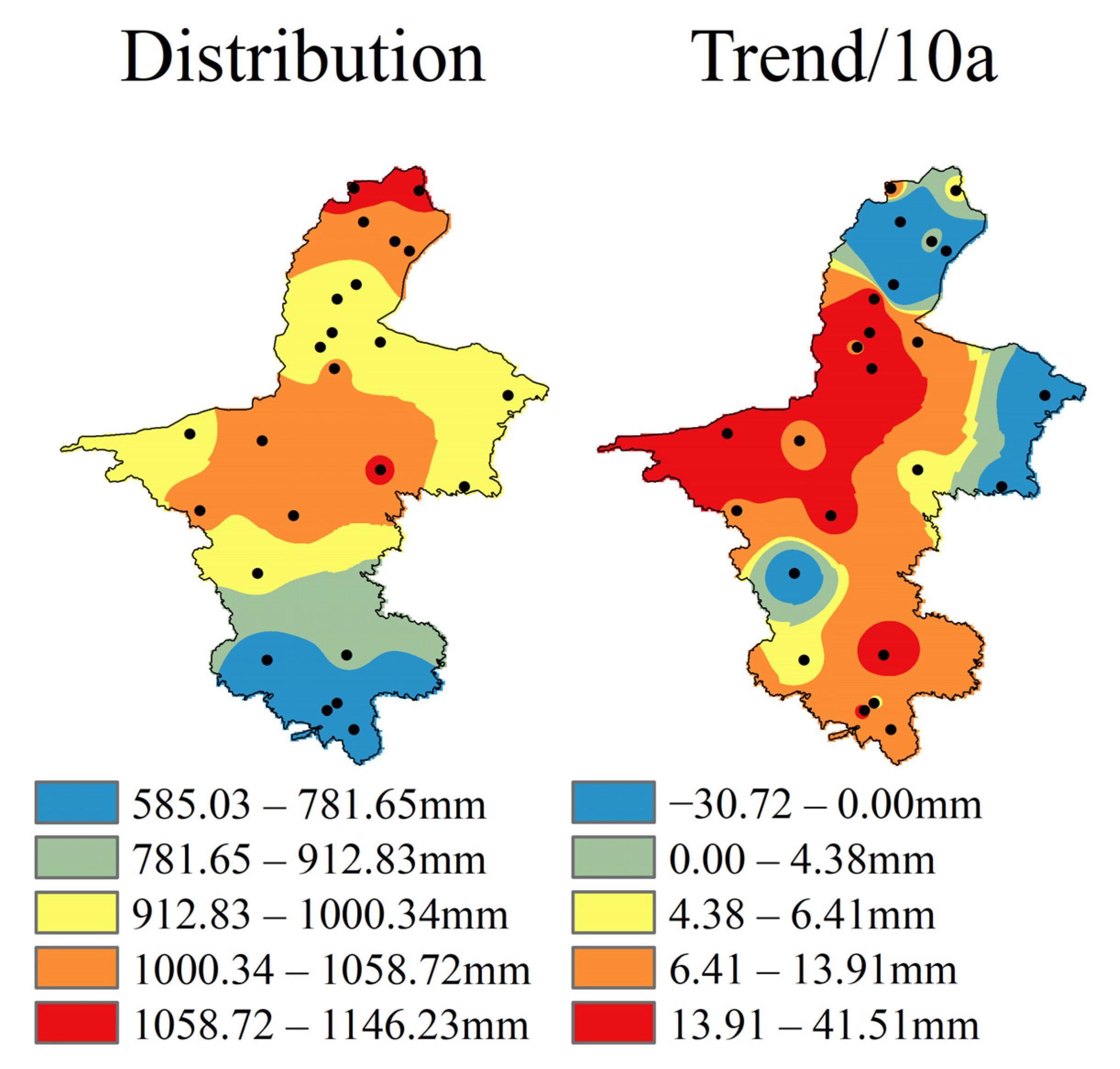
The spatial characteristics of potential evaporation in the growing season of Ningxia Autonomous Region are shown in Figure 2. The potential evaporation in Ningxia is between 585.03 mm and 1146.23 mm, with the potential evaporation in the middle of the central arid zone and in the north side of the northern region being larger, between 1000.34 and 1146.23 mm, and the potential evaporation in the southern region smaller, between 585.03 and 781.65 mm. The west side of the central region of Ningxia Hui Autonomous Region demonstrates a greater increasing trend, and its value is between 13.91 and 41.51. There is a decreasing trend in the east and north sides of Ningxia Hui Autonomous Region, and the decreasing trend is between −30.72 and 0.00 mm.

3.1.2. Monthly Potential Evaporation Distribution and Trend in the Growing Season

The monthly spatial characteristics of the potential evaporation in the growing season of Ningxia Autonomous Region are shown in Figure 3. The distribution of the potential evaporation in each month is exemplified by the potential evaporation in the central region and the northern region being larger, and the potential evaporation in the southern region being smaller. The potential evaporation continued to increase in June, and reached its largest value in June, with a value between 103.32 and 209.32 mm. The potential evaporation continued to decrease from July to October, and the potential evaporation in October was the smallest, with a value between 52.57 and 86.65 mm. The increasing trend of potential evaporation from April to June is relatively obvious, and the areas with a greater increasing trend are mainly concentrated in the west of the central region. The north of the northern region and the east of the central region have a decreasing trend. From July to October, the potential evaporation has a decreasing trend. The decreasing trend in September is the most obvious, but most areas show a decreasing trend to some extent. The northern part of the northern region and the eastern part of the central region have the largest decreasing trend, and the value is between −7.58 and −3.54.

3.1.3. Time Evolution Trend and Mutation of Potential Evaporation

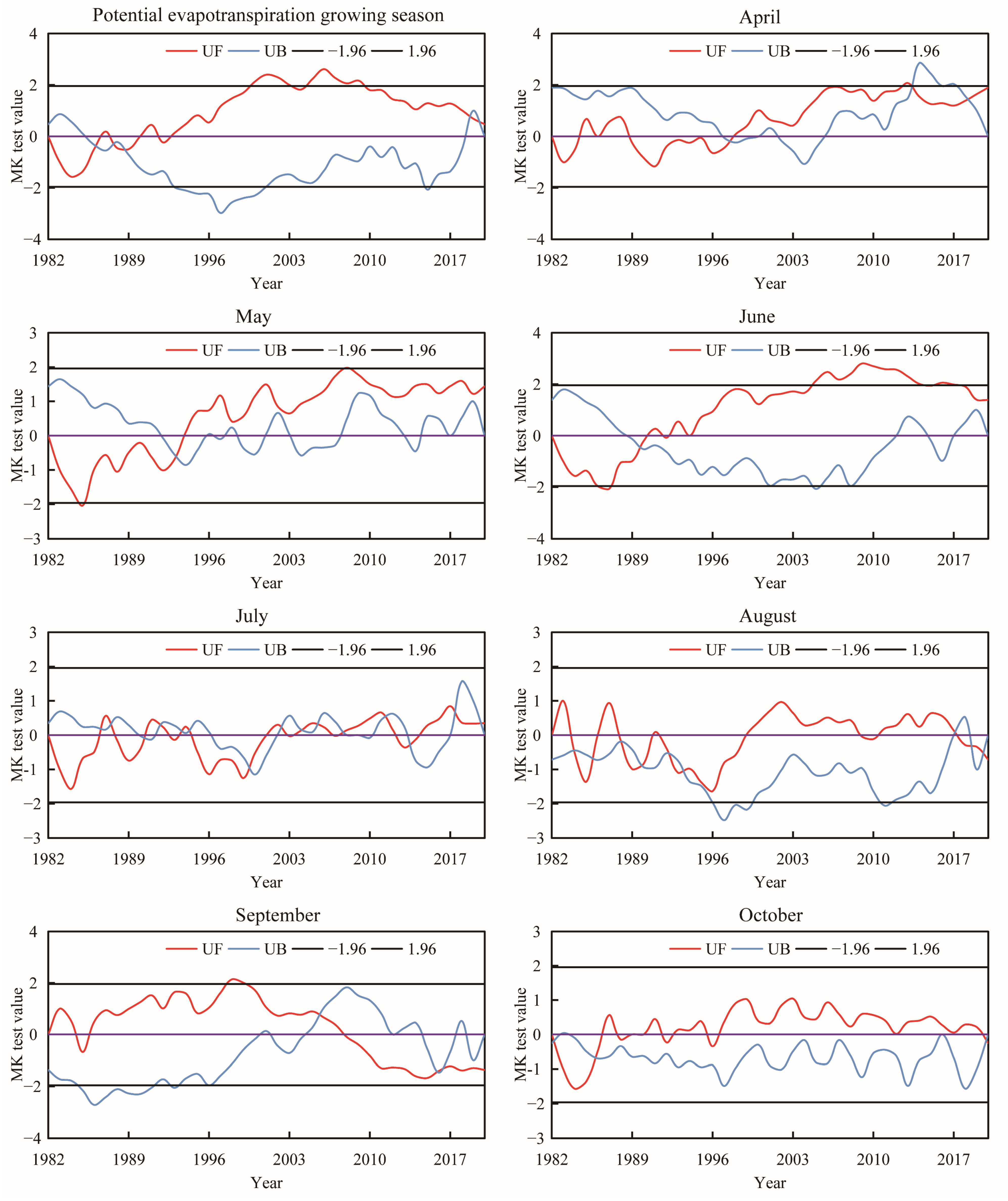
The temporal change law of potential evaporation (ET0) in Ningxia Hui Autonomous Region is shown in Figure 4. The UF value shows an “increase–decrease” trend on the time scale of the growing season. There is a downward trend in 2020, but the UF value greater than 0 indicates that the potential evaporation in the growing season is still rising, although the rising trend is decreasing. The mutation point appeared in 1988. From April to June, 1992–2020, the UF value showed an increasing trend. During this period, the potential evaporation increased. The mutation points appeared in 1998, 1993, and 1990, and appeared more frequently in July and August during the period from 1982 to 2020. At the mutation point, the change in UF value is relatively stable, and the increase in potential evaporation is not obvious. In September, the potential evaporation showed a downward trend from 1998 to 2020, and the mutation point appeared in 2005. The mutation point in October appeared in 1986, and the UF value changed. According to the results of the MK test, the potential evaporation in April, May, and June showed an increasing trend over the past 30 years, the UF value and potential evaporation in July, August, and October were relatively stable, and the potential evaporation in September showed a decline over the past 20 years.

3.2. Prediction of Potential Evaporation

3.2.1. Factor Screening and Model Construction

Pearson correlation analysis was carried out to assess the potential evaporation in the growing season and the circulation index combined in different time periods (shown in Table 1). Because the growing season is from April to October, the forecast factor was selected from April of the previous year. Using the circulation factor from March of that year, 1560 correlation coefficients were actually obtained. On this basis, factor screening was carried out. The correlation analysis between the atmospheric circulation index at different time periods and the potential evaporation in the growing season was carried out. After screening, 33 correlation coefficients were finally obtained at the 0.05 significance level. Atmospheric circulation factors and time periods were tested, of which nine circulation indices met the 0.01 significance level.

3.2.2. Establishment and Verification of the Potential Evaporation Prediction Model in the Growing Season

Based on the atmospheric circulation index factors in Table 1, the stepwise regression model was used to build the model. The model with a variance inflation factor (VIF) less than 5 was selected. Table 2 shows, The variance inflation factor of all models was within 2. The selected atmospheric circulation index factors were from April of the previous year to March of the current year.

3.2.3. Fitting Back-Generation of Potential Evaporation in the Growing Season

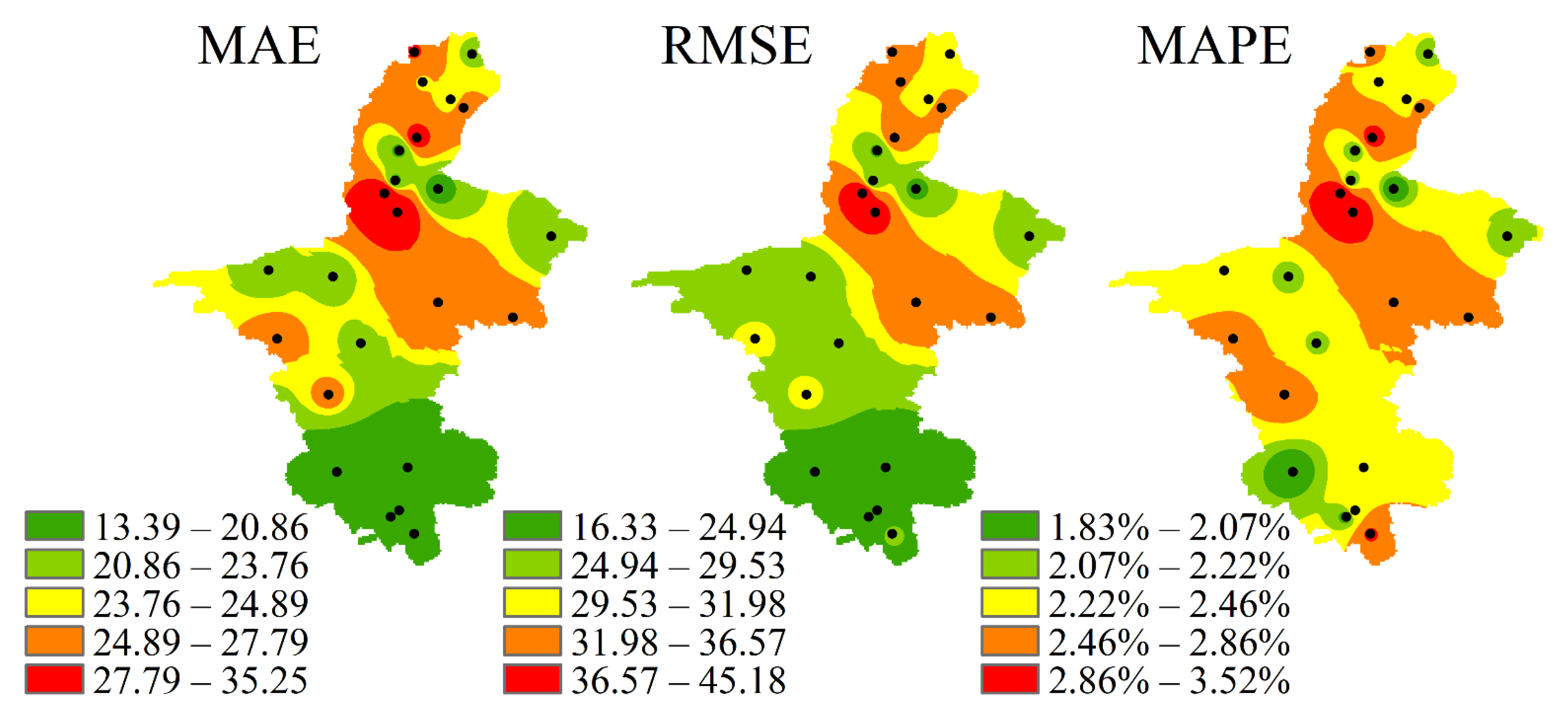
The potential evaporation during the growing season in Ningxia is between 585.16 and 1142.81 mm. As shown in Figure 5, the maximum actual value of potential evaporation (1055.85 to 1142.81 mm) is mainly distributed in the north of the northern part of Ningxia and the center of the central Ningxia arid zone. The potential evaporation in the growing season is between 585.14 and 1154.87 mm, and the predicted maximum potential evaporation is between 1062.75 and 1154.87 mm. The predicted potential evaporation distribution is basically consistent with the actual potential evaporation distribution. As shown in the error analysis in Figure 6, the mean absolute error (MAE) is between 13.39 and 35.25, the root mean square error (RMSE) is between 16.33 and 45.18, and the mean absolute percentage error (MAPE) is between 1.83% and 3.52%.

3.2.4. Extrapolated Forecast of Potential Evaporation during the Growing Season

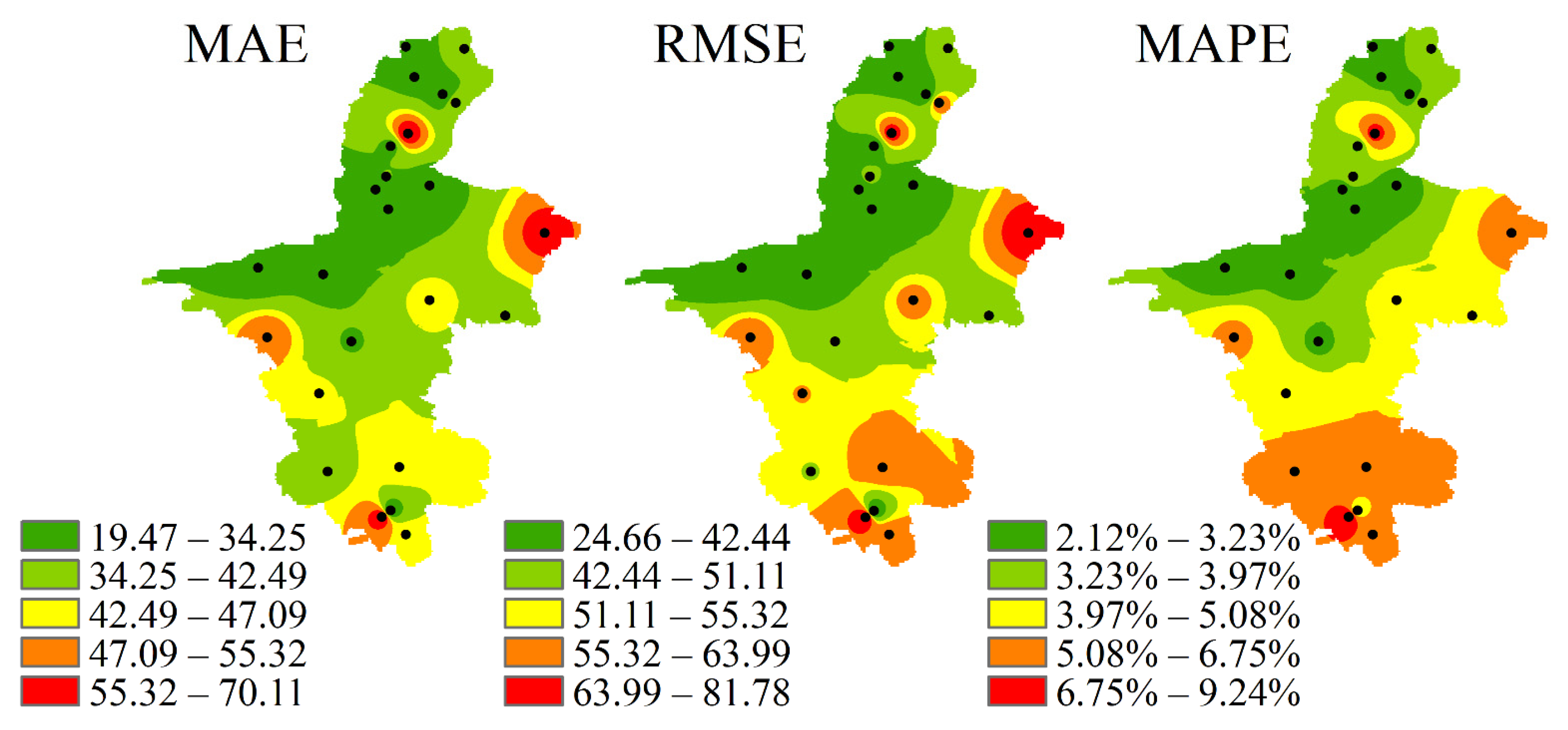
Figure 7 shows the distribution of the extrapolated forecast and the actual value, as well as the difference between the two. By comparing the distribution of the actual value and the predicted value from 2016 to 2020, although the potential evaporation has space and time differences, the predicted result is basically consistent with the actual value of the potential evaporation. The difference between the actual value and the predicted value in Ningxia is between −57.32 and 136.98. Through the error analysis of the extrapolated predictions in Figure 8, the mean absolute error (MAE) is between 19.47 and 70.11. The distribution of root mean square error (RMSE) and mean absolute error (MAE) is roughly consistent, and the root mean square error (RMSE) in Ningxia is between 24.66 and 81.78. The mean absolute percentage error (MAPE) of all regions is within 10%, among which the northern region (green region) has the smallest error, between 2.12 and 3.97%, and the southern region has a larger prediction error.

3.2.5. Monthly Fitting Back-Generation of Potential Evaporation in the Growing Season

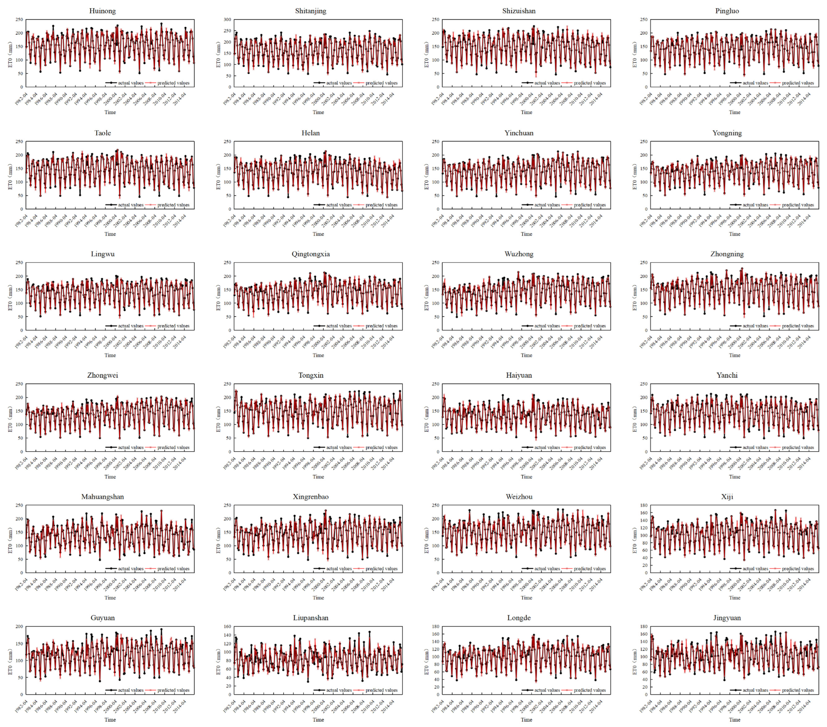
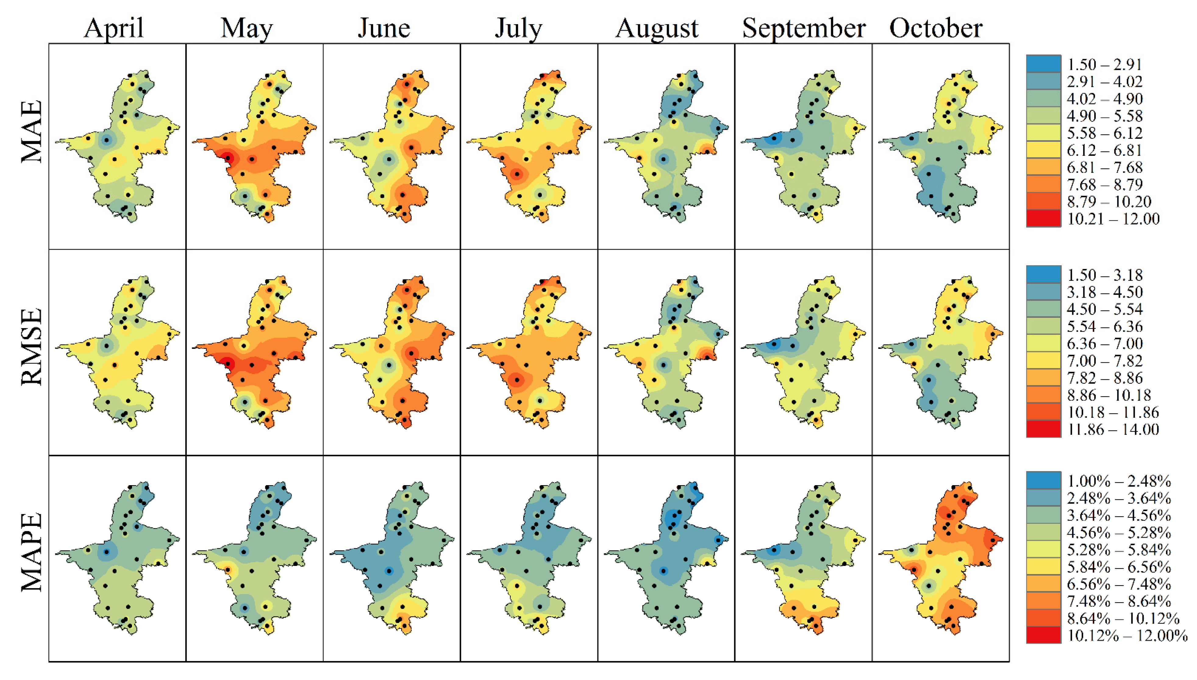
Based on the circulation factor, a monthly potential evaporation prediction model is established, and the model is established by using a circulation factor that is pushed 12 months ahead of the predicted month. The modeling steps are consistent with the potential evaporation in the growing season, and collinearity (VIF) less than 5 is selected. The basic information of the selected model is shown in Table 3 and Table 4. Models, due to space reasons, are no longer listed one by one. According to Figure 9, the fitted values from 1982 to 2015 are basically consistent with the actual values. As shown in Figure 10, the mean absolute error (MAE) is generally between 1.50 and 12.00 in each month, and the red area is larger in May, June, and July, indicating that the mean absolute error (MAE) error is larger; the blue areas are larger in August, September, and October, indicating a smaller mean absolute error (MAE). The root mean square error (RMSE) is generally between 1.50 and 14.00 in each month, and the red area is larger in May, June, and July, indicating that the root mean square error (RMSE) is larger. On the other hand, the blue area in August, September, and October is larger, and the root mean square error (RMSE) is small. The mean absolute percentage error (MAPE) is between 1.00% and 12.00% across all months as a whole. In October, the red area is larger, indicating that the mean absolute percentage error (MAPE) is larger; in August, the blue area is larger, indicating that the mean absolute percentage error (MAPE) is smaller.

3.2.6. Monthly Extrapolation Forecast of Potential Evaporation in the Growing Season

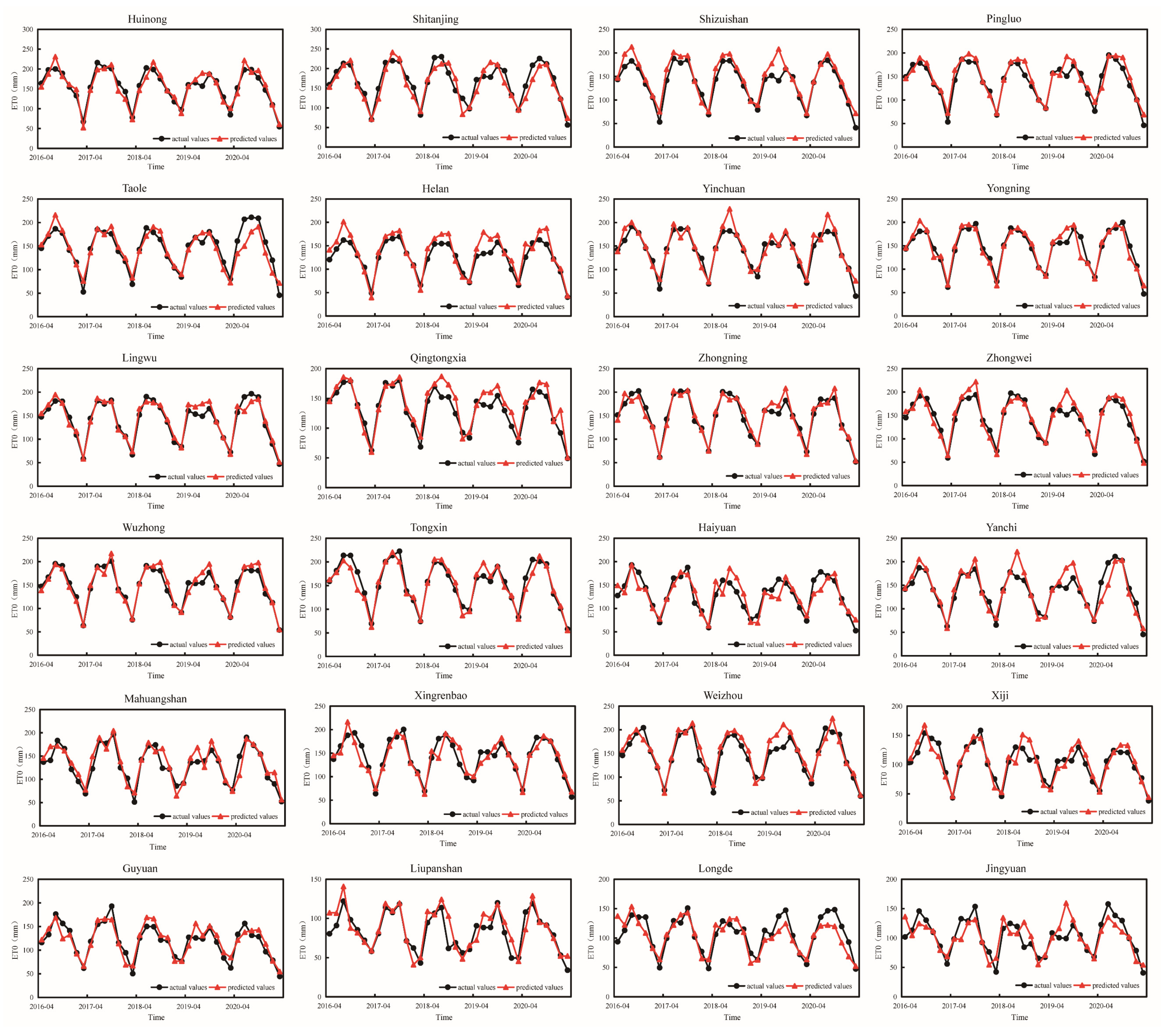
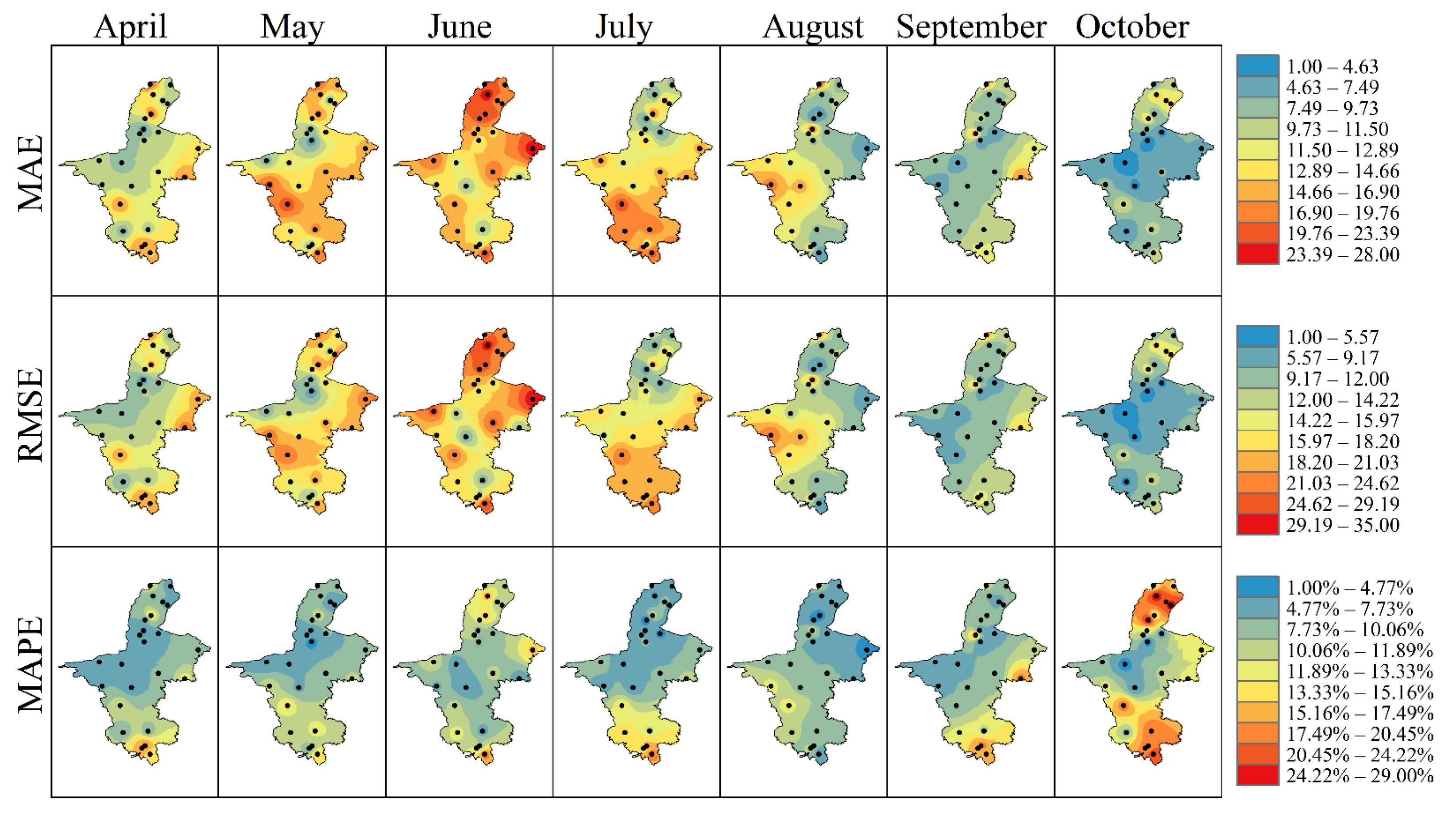
The monthly forecast and actual values of various regions in Ningxia from 2016 to 2020 are essentially the same, as shown in Figure 11. As shown in Figure 12, the overall range of the mean absolute error (MAE) is between 1.00 and 28.00, and the months with larger red areas are May, June, and July, indicating that the mean absolute error (MAE) is larger. The months with larger blue areas are September and October, indicating that the mean absolute error (MAE) is small. The overall range of the root mean square error (RMSE) is between 1.00 and 35.00, and the distribution is basically consistent with the mean absolute error (MAE). The mean absolute percentage error (MAPE) is mainly between 1.00% and 29.00%. In October, the error is relatively large, with more red areas. Regarding the other months, most are in the yellow area and the blue area (between 1% and 15.16%), with the smallest mean absolute percentage error (MAPE) in August.

4. Discussion

Evaporation is a bridge in terms of land–atmosphere interactions, and plays an extremely important role in the hydrological cycle and agricultural irrigation [20]. The atmospheric circulation has a strong influence on the potential evaporation in the growing season [21]. Its drastic change has led to the acceleration of the water cycle [22], which has also affected potential evaporation. Previous studies have found that the Arctic Oscillation (AO) is closely related to the mid-to-high latitudes [23], and some studies have shown that the hydrological cycle is important for El Niño Southern Toss. This is closely related to cyclones (NHPV), the Atlantic Oscillation (ENSO), and the North Atlantic Oscillation (NAO) [24], which may affect the change in evaporation through the circulation anomaly, and then affect the occurrence of meteorological and hydrological drought [25]. Other studies have shown that China’s climate is mainly affected by the synchronous subtropical high in the western North Pacific and the atmospheric circulation in the mid-to-high latitudes of the North Pacific, as well as the monsoon circulation in the western North Pacific [26,27].
This study describes the temporal and spatial relationship of potential evaporation in the growing season, and uses the step-by-step asymptotic regression method to predict the potential evaporation in the growing season. The results show that the potential evaporation in the growing season from 1990 to 2010 has a larger increasing trend, which is consistent with the fifth IPCC assessment report [28], which provides the conclusion that 1983–2012 was the hottest 30-year period in the past 1400 years. The spatiotemporal analysis of potential evaporation in the growing season shows that the potential evaporation in April, May, and June has shown an increasing trend over the past 30 years. The UF value in July, August, and October was relatively stable, and the potential evaporation was relatively stable. The potential evaporation in September has shown a downward trend over the past 20 years. The prediction results show that the predicted value of the potential evaporation in the growing season is basically consistent with the actual value, the predicted actual value of the potential evaporation in the growing season is basically consistent with the predicted value curve, and the mean absolute percentage error (MAPE) in October is relatively large. The mean absolute error (MAE) and root mean square error (RMSE) in June were larger.

5. Conclusions

Potential evaporation is an important factor in both the hydrological cycle and farmland irrigation. Based on the daily data of 24 meteorological stations, this paper analyzes the time series changes in potential evaporation during the growing season in Ningxia, and systematically establishes a prediction model of potential evaporation during this period. The hydrological cycle change and farmland irrigation system in Ningxia in the growing season are used to provide a reference. The main conclusions are as follows:
(1)
The areas with large potential evaporation in the growing season are mainly the central area and the northern side of the northern area of Ningxia. The western side of the central area of the Ningxia Hui Autonomous Region has a greater increasing trend, and the eastern and northern sides of the Ningxia Hui Autonomous Region have a decreasing trend.
(2)
On the monthly scale, the potential evaporation continued to increase from April to June, reached its maximum in June, continued to decrease from July to October, and was the smallest in October. The increasing trend of potential evaporation from April to June and the increasing trend of the west side of the central region are obvious, and the trend of potential evaporation from July to October is more obvious, during which the decreasing trend is most obvious in September, although most areas show a decrease to some extent. Among them, the northern side of the northern region and the eastern side of the central region have the largest decreasing trend.
(3)
According to the results of the MK test in the growing season, the change in potential evaporation in the growing season showed a trend of “increase–decrease”. According to the results of the monthly scale MK test, the potential evaporation in April, May, and June has shown an increasing trend over the past 30 years. The UF value in August and October has been relatively stable, and the trend of potential evaporation has been relatively stable. The potential evaporation in September has shown a downward trend over the past 20 years.
(4)
The prediction model of potential evaporation in the growing season established by atmospheric circulation has shown good results in Ningxia, demonstrating that the circulation factor can be used to establish the scheduling forecast for irrigation water.

Author Contributions

This paper was calculated and written by Z.L., guided by Q.S., and revised and discussed by D.X., W.F., R.W. and P.J. All authors have read and agreed to the published version of the manuscript.

Funding

This study was funded by the National Key Research and Development Program “Research and Demonstration of Key Technologies for the Wine Industry in the Eastern Helan Mountains of Ningxia” (2019YFD1002502).

Institutional Review Board Statement

Not applicable.

Informed Consent Statement

All subjects involved in this study provided informed consent.

Data Availability Statement

Not applicable.

Acknowledgments

Thanks are given to the National Meteorological Center of China Meteorological Administration for providing the meteorological and index datasets.

Conflicts of Interest

The authors declare no conflict of interest.

References

  1. Allen, R.G.; Pereira, L.S.; Smith, M.; Raes, D.; Wright, J.L. FAO-56 dual crop coefficient method for estimating evaporation from soil and application extensions. J. Irrig. Drain. Eng. 2005, 131, 2–13. [Google Scholar] [CrossRef] [Green Version]
  2. Singh, V.P. Volume I: Rainfall-runoff modeling. In Hydrologic Systems; Prentice Hall: Englewood Cliffs, NJ, USA, 1988; p. 480. [Google Scholar]
  3. Jaramillo, F.; Prieto, C.; Lyon, S.W.; Destouni, G. Multimethod assessment of evapotranspiration shifts due to non-irrigated agricultural development in Sweden. J. Hydrol. 2013, 484, 55–62. [Google Scholar] [CrossRef] [Green Version]
  4. Qin, D.; Chen, Z.; Averyt, K.B.; Miller, H.L.; Solomon, S.; Manning, M.; Marquis, M.; Tignor, M. IPCC, 2007: Summary for Policymakers; Cambridge University Press: Cambridge, UK, 2007. [Google Scholar]
  5. Waller, P.; Yitayew, M. Crop Evapotranspiration. In Irrigation and Drainage Engineering; Springer: Cham, Switzerland, 2016; pp. 89–104. [Google Scholar]
  6. Duce P, Snyder R L, Spano D. Forecasting reference evapotranspiration. In Proceedings of the III International Symposium on Irrigation of Horticultural Crops, Lisbon, Portugal, 1 October 2000.
  7. Li, L.; Ni, W.; Li, Y.; Guo, D.; Gao, H. Impacts of Sea Surface Temperature and Atmospheric Teleconnection Patterns in the Northern Mid-Latitudes on Winter Extremely Cold Events in North China. Adv. Meteorol. 2021, 2021, 853457. [Google Scholar] [CrossRef]
  8. Xu, J.; Li, F. Response of lower Yellow River bank breachings to La Nia events since 924CE. Catena 2019, 176, 159–169. [Google Scholar] [CrossRef]
  9. Gritsun, A.S. Variability of extra tropical atmospheric circulation and periodic trajectories in simplified models of atmospheric dynamics. Izv. Atmos. Ocean. Phys. 2020, 56, 229–240. [Google Scholar] [CrossRef]
  10. Kyselý, J. Implications of enhanced persistence of atmospheric circulation for the occurrence and severity of temperature extremes. Int. J. Climatol. A J. R. Meteorol. Soc. 2007, 27, 689–695. [Google Scholar] [CrossRef]
  11. Schubert, S.; Rienecker, M.; Mlynczak, M.; Miller, T.; Schoeberl, M. Ocean and atmosphere: Predicting monthly to seasonal climate variability and the oceanic and atmospheric causes and effects. In Proceedings of the IGARSS 2003. 2003 IEEE International Geoscience and Remote Sensing Symposium, Toulouse, France, 21–25 July 2003; IEEE: Piscataway, NJ, USA, 2003; Volume 1, pp. 142–144. [Google Scholar]
  12. Jackson, L.C.; Smith, R.S.; Wood, R.A. Ocean and atmosphere feedbacks affecting AMOC hysteresis in a GCM. Clim. Dyn. 2017, 49, 173–191. [Google Scholar] [CrossRef] [Green Version]
  13. Zheng, J.; Li, B.; Chen, Y.; Chen, Z.; Lian, L. Spatiotemporal variation of upper-air and surface wind speed and its influencing factors in northwestern China during 1980–2012. Theor. Appl. Climatol. 2017, 133, 1303–1314. [Google Scholar] [CrossRef]
  14. Kononova, N.K.; Lupo, A.R. Changes in the Dynamics of the Northern Hemisphere Atmospheric Circulation and the Relationship to Surface Temperature in the 20th and 21st Centuries. Atmosphere 2020, 11, 255. [Google Scholar] [CrossRef] [Green Version]
  15. Po-Chedley, S.; Zelinka, M.D.; Jeevanjee, N.; Thorsen, T.J.; Santer, B.D. Climatology explains intermodel spread in tropical upper tropospheric cloud and relative humidity response to greenhouse warming. Geophys. Res. Lett. 2019, 46, 13399–13409. [Google Scholar] [CrossRef]
  16. Urban, G.; Migała, K.; Pawliczek, P. Sunshine duration and its variability in the main ridge of the Karkonosze Mountains in relation to with atmospheric circulation. Theor. Appl. Climatol. 2018, 131, 1173–1189. [Google Scholar] [CrossRef] [Green Version]
  17. Ahmadi, S.H.; Fooladmand, H.R. Spatially distributed monthly reference evapotranspiration derived from the calibration of Thornthwaite equation: A case study, South of Iran. Irrig. Sci. 2008, 26, 303–312. [Google Scholar] [CrossRef]
  18. Heydari, M.M.; Heydari, M. Calibration of Hargreaves–Samani equation for estimating reference evapotranspiration in semiarid and arid regions. Arch. Agron. Soil Sci. 2014, 60, 695–713. [Google Scholar] [CrossRef]
  19. Heydari, M.M.; Tajamoli, A.; Ghoreishi, S.H.; Darbe-Esfahani, M.K.; Gilasi, H. Erratum to: Evaluation and calibration of Blaney–Criddle equation for estimating reference evapotranspiration in semiarid and arid regions. Environ. Earth Sci. 2015, 74, 4053–4063. [Google Scholar] [CrossRef]
  20. Xu, Y.P.; Pan, S.; Fu, G.; Tian, Y.; Zhang, X. Future potential evapotranspiration changes and contribution analysis in Zhejiang Province, East China. J. Geophys. Res. D Atmos. Jgr. 2014, 119, 2174–2192. [Google Scholar] [CrossRef] [Green Version]
  21. Sun, H.; Hu, H.; Wang, Z.; Lai, C. Temporal Variability of Drought in Nine Agricultural Regions of China and the Influence of Atmospheric Circulation. Atmosphere 2020, 11, 990. [Google Scholar] [CrossRef]
  22. Willems, P. Compound intensity/duration/frequency-relationships of extreme precipitation for two seasons and two storm types. J. Hydrol. 2000, 233, 189–205. [Google Scholar] [CrossRef]
  23. Hudgins, L. Bivariate wavelet analysis of Asia monsoon and ENSO. Adv. Atmos. Sci. Engl. Version 1996, 13, 299–312. [Google Scholar] [CrossRef]
  24. Talaee, P.H.; Tabari, H.; Ardakani, S.S. Hydrological drought in the west of Iran and possible association with large-scale atmospheric circulation patterns. Hydrol. Processes 2014, 28, 764–773. [Google Scholar] [CrossRef]
  25. Huang, S.; Li, P.; Huang, Q.; Leng, G.; Hou, B.; Ma, L. The propagation from meteorological to hydrological drought and its potential influence factors. J. Hydrol. 2017, 547, 184–195. [Google Scholar] [CrossRef]
  26. Liu, Y. Influence of the Western North Pacific Summer Monsoon on Summer Rainfall over the Yangtze River Basin. Chin. J. Atmos. Sci. 2009, 33, 1225–1237. [Google Scholar]
  27. Zhang, Q.Y.; Tao, S.Y. Tropical and subtropical monsoon over east asia and its influence on the rainfall over eastern china in summer. Q. J. Appl. Meteorl. 1998, 9, 17–23. [Google Scholar]
  28. Climate Change 2013: The Physical Science Basis; Working Group I Contribution to the Fifth Assessment Report of the Intergovernmental Panel on Climate Change; Cambridge University Press: New York, NY, USA, 2013; Available online: https://www.ipcc.ch/site/assets/uploads/2017/09/WG1AR5_Frontmatter_FINAL.pdf (accessed on 10 August 2022).
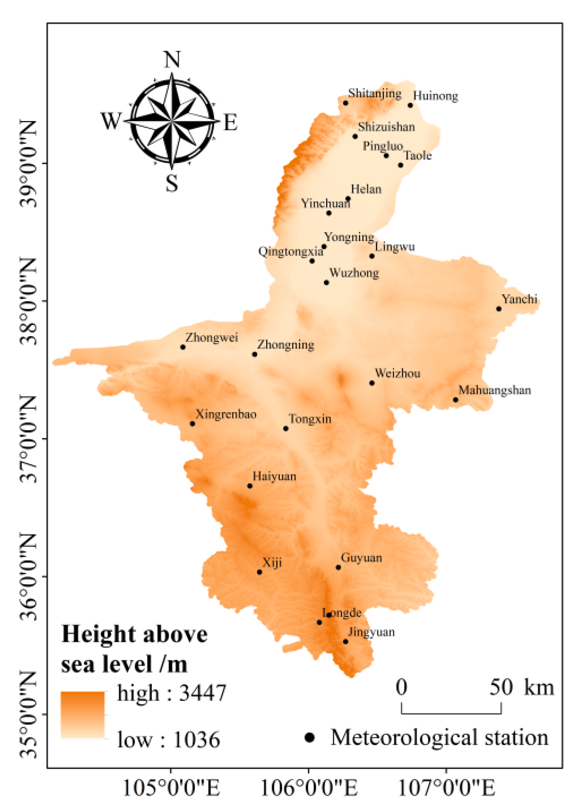
Figure 1. Altitude and distribution of meteorological stations in Ningxia.
Atmosphere 13 01654 g001
Figure 2. Spatial characteristics of potential evaporation during the growing season in Ningxia Autonomous Region.
Atmosphere 13 01654 g002
Figure 3. Spatial characteristics of monthly potential evaporation during the growing season in Ningxia Autonomous Region.
Atmosphere 13 01654 g003
Figure 4. Monthly MK test values of potential evaporation during the growing season.
Atmosphere 13 01654 g004
Figure 5. The annual average distribution of the actual and predicted values of the fitted back-alternative.
Atmosphere 13 01654 g005
Figure 6. Fitting back-substitution error analysis (mean absolute error (MAE), root mean square error (RMSE), and mean absolute percentage error (MAPE)).
Atmosphere 13 01654 g006
Figure 7. Distribution of and differences between actual and predicted values, unit/mm (Va is the actual value from 2016 to 2020, Vp is the predicted value from 2016 to 2020, and Va-Vp is the actual value minus the predicted value).
Atmosphere 13 01654 g007
Figure 8. Analysis of extrapolated forecast error, mean absolute error (MAE), root mean square error (RMSE), and mean absolute percentage error (MAPE).
Atmosphere 13 01654 g008
Figure 9. The Ningxia area fitted with back-generation.
Atmosphere 13 01654 g009
Figure 10. Error analysis of fitted values: mean absolute error (MAE), root mean squared error (RMSE), and mean absolute percentage error (MAPE).
Atmosphere 13 01654 g010
Figure 11. Monthly extrapolated predicted values of potential evaporation in various regions of Ningxia.
Atmosphere 13 01654 g011
Figure 12. Extrapolated forecast error analysis: mean absolute error (MAE), root mean squared error (RMSE), and mean absolute percentage error (MAPE).
Atmosphere 13 01654 g012
Table 1. Correlation analysis was carried out for potential evaporation in the growing season (April–October) with a time lag of 12 months (April–December of the previous year and January–March of the current year), and a significant p was selected. Atmospheric circulation factor < 0.05.
TimeNumberingIndex NameCorrelationTimeNumberingIndex NameCorrelation
April of the previous yearX1Northern Hemisphere Polar Vortex Central Intensity Index0.338 *September of the previous yearX19Western Pacific Subtropical High Northern Boundary Position Index−0.345 *
April of the previous yearX2Western North Pacific Typhoon number0.348 *September of the previous yearX20Asian Zonal Circulation Index0.318 *
May of the previous yearX3Eastern Pacific Subtropical High Northern Boundary Position Index−0.394 *September of the previous yearX21North Atlantic Triple index−0.340 *
May of the previous yearX4Asia Polar Vortex Area Index−0.440 **October of the previous yearX22Western North Pacific Typhoon number−0.319 *
May of the previous yearX5Northern Hemisphere Polar Vortex Central Longitude Index−0.318 *November of the previous yearX23Indian Subtropical High Ridge Position Index0.327 *
May of the previous yearX6Central Pacific 850 mb Trade Wind Index0.322 *November of the previous yearX24Northern Hemisphere Polar Vortex Area Index−0.318 *
June of the previous yearX7North African–North Atlantic–North American Subtropical High Ridge Position Index0.525 **November of the previous yearX25East Atlantic–West Russia Pattern, EA/WR−0.393 *
June of the previous yearX8North American Subtropical High Northern Boundary Position Index0.343 *December of the previous yearX26Atlantic Subtropical High Ridge Position Index0.419 **
June of the previous yearX9Western Pacific Subtropical High Western Ridge Point Index0.318 *January of that yearX27Western Pacific Subtropical High Ridge Position Index−0.411 **
June of the previous yearX10Western Pacific Warm Pool Area Index0.323 *January of that yearX28Pacific Subtropical High Ridge Position Index−0.332 *
July of the previous yearX11Asia Polar Vortex Area Index−0.421 **February of that yearX29Asian Zonal Circulation Index0.332 *
July of the previous yearX12Northern Hemisphere Polar Vortex Central Latitude Index0.418 **February of that yearX30South Indian Ocean Dipole Index0.536 **
July of the previous yearX13East Asian Trough Intensity Index0.379 *March of that yearX31East Asian Trough Position Index−0.362 *
August of the previous yearX14North American Subtropical High Ridge Position Index−0.491 **March of that yearX32Polar–Eurasia Pattern, POL−0.320 *
August of the previous yearX15Western Pacific Subtropical High Western Ridge Point Index−0.389 *March of that yearX33South Indian Ocean Dipole Index0.474 **
August of the previous yearX16Northern Hemisphere Polar Vortex Central Longitude Index−0.319 *
Last augustX17East Pacific 850 mb Trade Wind Index−0.404 *
Last augustX18Oyashio Current SST Index0.342 *
* The correlation is significant at the 0.05 level, ** the correlation is significant at the 0.01 level.
Table 2. Models built based on the atmospheric circulation index. Stepwise regression was used to select a suitable model through the expansion factor test (VIF < 10).
CityModel FormulasVariance Inflation Factor
Huinongy = 1438.701 + 6.856 × 7 + 0.64 × 9 − 8.158 × 11 − 15.609 × 14X7X9X11X14
1.2631.131.0381.091
Shizuishany = 1675.5 − 0.03 × 3 − 13.094 × 10 − 21.89 × 27 + 51.134 × 30X3X10X27X30
1.0421.1181.0591.088
Yinchuany = 672.282 + 0.224 × 1 + 6.772 × 10 − 18.617 × 14 − 5.996 × 24 + 0.039 × 26 + 17.952 × 33X1X10X14X24X26X33
1.321.4731.1261.2391.2891.196
Shitanjingy = −1377.114 + 0.114 × 13 − 23.61 × 14 + 33.532 × 33X13X14X33
1.3141.0451.295
Pingluoy = 311.32 + 0.228 × 1 − 17.432 × 14 + 5.104 × 29 + 23.766 × 30X1X14X29X30
1.0711.0341.1221.179
Taoley = 1497.921 − 0.029 × 3 − 21.713 × 4 − 8.443 × 11 + 28.622 × 30X3X4X11X30
1.0481.0371.1921.17
Helany = 1969.009 − 0.049 × 03 − 42.471 × 04 − 3.861 × 12 − 0.084 × 19 + 43.525 × 30X3X4X12X19X30
1.0461.2451.6391.1091.245
Yongningy = 1544.971 − 13.188 × 14 − 0.176 × 16 − 16 × 17 + 10.35 × 18 + 0.038 × 26 + 22.343 × 33X14X16X17X18X26X33
1.1631.21.3061.3091.2771.262
Lingwuy = 621.255 + 0.175 × 1 + 0.447 × 9 − 17.038 × 14 − 9.442 × 17 + 19.333 × 33X1X9X14X17X33
1.1511.0891.0921.1821.097
Qingtongxiay = 1292.535 − 25.765 × 28 + 9.383 × 29 − 73.376 × 32X28X29X32
1.0261.041.033
Wuzhongy = 1407.758 − 36.337 × 4 + 16.279 × 10 − 34.602 × 17 + 9.421 × 20X4X10X17X20
1.011.1681.0681.095
Zhongningy = 1498.873 + 0.673 × 09 − 11.268 × 14 − 11.659 × 28 + 45.472 × 30 − 32.359 × 32X9X14X28X30X32
1.0441.131.1221.011.035
Zhongweiy = 1935.119 + 4.937 × 8 + 8.996 × 10 − 18.349 × 17 − 6.358 × 24 − 18.253 × 27 − 2.936 × 31X8X10X17X24X27X31
1.1541.3831.1771.2621.1651.351
Tongxiny = 2019.003 − 16.043 × 14 − 0.614 × 15 − 0.185 × 16 − 5.315 × 24 + 22.342 × 33X14X15X16X24X33
1.1561.1771.1641.1531.201
Xijiy = 789.801 + 17.915 × 2 − 0.038 × 3 − 0.072 × 19 − 20.455 × 21 − 0.659 × 31 + 13.386 × 33X02X03X19X21X31X33
1.0941.1711.1961.4651.1651.167
Haiyuany = 947.905 + 29.972 × 2 − 0.035 × 3 − 0.376 × 15 + 23.52 × 33X2X3X15X33
1.0741.0751.2231.198
Yanchiy = 1398.19 − 0.03 × 3 − 21.875 × 4 − 0.435 × 15 − 0.044 × 19 + 43.928 × 25 + 39.461 × 30X3X4X15X19X25X30
1.0391.1381.4641.2061.551.559
Mahuangshany = 1067.008 + 34.322 × 2 + 0.933 × 9 + 4.036 × 12 − 16.849 × 27 + 44.168 × 30 − 2.102 × 31X2X9X12X27X30X31
1.081.0891.241.0531.281.11
Xingrenbaoy = 2114.237 − 8.852 × 11 − 17.166 × 14 − 6.311 × 24 + 0.058 × 26 + 23.573 × 33X11X14X24X26X33
1.2481.0951.1321.1141.199
Weizhouy = 435.339 + 0.237 × 1 + 0.672 × 9 − 21.703 × 14 + 31.121 × 33X1X9X14X33
1.11.0121.0321.085
Guyuany = −1877.545 − 0.047 × 3 + 0.112 × 13 − 0.197 × 15 − 0.073 × 19 − 24.972 × 21 − 6.885 × 24X03X13X15X19X21X24
1.0661.4681.241.3511.8271.145
Liupanshany = 945.127 + 12.909 × 2 − 14.132 × 14 − 0.062 × 19 + 4.85 × 29 − 29.462 × 30 + 34.969 × 33X2X14X19X29X30X33
1.1921.2261.131.1464.6174.283
Longdey = 1004.488 − 0.031 × 3 − 14.066 × 4 − 9.009 × 17 − 0.078 × 19 − 18.702 × 21 + 17.085 × 30X3X4X17X19X21X30
1.2591.1061.3371.2391.7411.237
Jingyuany = 1040.664 + 20.605 × 2 − 10.903 × 14 − 0.089 × 19 + 0.05 × 26 + 27.748 × 33X2X14X19X26X33
1.1491.11.0361.0381.042
Table 3. Number of selected circulation index factors (correlation significant p < 0.05).
AprilMayJuneJulyAugustSeptemberOctober
12713870366210088
Table 4. Stepwise asymptotic regression to select the number of factors (VIF < 10).
PlaceAprilMayJuneJulyAugustSeptemberOctober
Huinong55541457
Shitanjing6563665
Shizuishan55310597
Pingluo7954575
Taole64761255
Helan4535758
Yinchuan67123954
Yongning665616107
Lingwu6546656
Qingtongxia6859845
Wuzhong45944137
Zhongning8855596
Zhongwei356841410
Tongxin941461357
Haiyuan561335510
Yanchi45551055
Mahuangshan5676495
Xingrenbao7364455
Weizhou5545786
Xiji5953427
Guyuan6549545
Liupanshan5853844
Longde81195555
Jingyuan6453837
Publisher’s Note: MDPI stays neutral with regard to jurisdictional claims in published maps and institutional affiliations.