Abstract
Climate change is perceived to be the primary reason for the amplification of extreme climatic phenomena. Estimation of changes in extreme values under climate change thus plays an important role in disaster risk assessment and management. However, the different changes in extremes in two distinct regions: inland and coast under climate change are yet to be investigated meticulously. This study is intended to assess the changes in frequency of rainfall and temperature extremes under the impact of climate change in two distinct locations: coast and inland of Bengal delta, a region highly vulnerable to climate change. The multi-model ensemble (projections from CMIP6 framework) technique with the application of frequency analysis was employed to appraise the impact in two future time horizons. Results suggest that the inland estimate of extreme rainfall by the end of this century is barely able to exceed the coastal estimate of extreme rainfall in present conditions. The rate of increase of warm extremes is almost similar; however, with the cold extreme, the increase rate is a little higher inland than on the coast. In both regions, a greater rise in climate extremes is expected in the far future than in the near future. Overall, the coastal area is expected to be more vulnerable to flooding while the inland to drought under climate change in the Bengal delta region.
1. Introduction
Climate change is perceived to be a major threat to the world [1,2]. Rapid increases in temperature under anthropogenic disturbances alter the hydrological cycle and change the rainfall pattern [2,3]. With the overall changes in climate, the phenomenon has the ability to modify extremes such as temperature and rainfall extremes, which have been recognized by the past studies with the observed data [4,5,6,7,8,9] and simulated future data [10,11,12,13,14,15]. Since abrupt changes in climate extremes lead to severe floods and droughts, studies on extremes have attracted global attention to planning and managing water resources.
The changes in extremes are, however, asymmetrical across the world. A large variation is perceived in frequency, spatial and temporal extent across different continents [4,5,10,11]. Scientists are thus encouraged to explore different territories of the world so that different changes can be reported, which would offer a different perspective. Coastal area is one important domain that is considered vulnerable to climate change [2,16,17,18,19,20]. It is understood that the spatiotemporal dynamics of disastrous occurrences may fluctuate significantly between coastal and inland locations due to differing physiographic and climatic environments. Despite the disparity, there has been only a limited effort to comprehend the differential pattern of extreme occurrences between coastal and inland regions under climate change. Temperature and rainfall extremes are identified as two climatic components that have a major impact on society and the environment [4,10,11]. Therefore, how these extremes behave in those areas under climate change is a matter of concern.
This study compares the effect of climate change on temperature and rainfall extremes (return period values) between coastal and inland regions of Bengal delta, territory which is highly vulnerable to climate change. The Bengal delta is unique in many ways [21,22]. It has Himalayan Mountains in the north and the Bay of Bengal in the south. The Bay of Bengal has a major influence on the climate of the coastal area and beyond. The monsoon is prominent, and it dominates the climate. The total discharge accumulating into the Ganges–Brahmaputra–Meghna basin flows through the delta. Due to this, the region, namely Bangladesh, is one of the most vulnerable places on earth to climate change [23,24]. Disasters such as floods and droughts cost the country over USD 3 billion between 1998 and 2014 [25]. It is estimated that overall crop production in Bangladesh is expected to fall by 7.4% per year from 2005 to 2050 due to extreme climatic events [26]. Thus, quantifying the changes in climatic extremes is essential for adaptation planning for the future.
However, the changes in rainfall and temperature extremes have not been properly understood in the changing setting of climate at the regional extent of Bengal delta. Even though significant work [21,27,28,29,30,31,32,33] has been performed in this region to investigate the characteristic changes in overall temperature and rainfall values, there has hardly been any attempt to quantify the combined assessment of changes of extreme temperature and rainfall under climate change. Additionally, relatively less effort has been invested to unearth the changes in extremes in Bangladesh’s coastal regions. The Bangladesh coast is considered to be the most climatically susceptible area, which is incessantly hit by tidal surges, cyclones and flooding [21]. The investigation of extremes in general explores either the changes in the observed trend [21] or the simulated indices [22]. A very limited study has been carried out to date to evaluate the temporal and spatial extent of rainfall and temperature extremes in the coastal area under various climatic scenarios, as adopted in the CMIP6 (Coupled Model Intercomparison Project Phase 6) framework, which is the region’s most vulnerable area to climate change and where the Bangladesh government is planning and implementing climate change adaptation strategies.
Thus, it is essential to examine the behavior of climate extremes at coastal locations and their deviation from the inland territory. Considering the interest in climate change worldwide, especially in connection with the changes in extremes in the regional context and their effects, the present work is intended to assess the changes in frequency of rainfall and temperature extremes under climate change in two distinct regional setups, namely coastal and inland locations. We investigate the changes in extremes by deriving projections from CMIP6 under multiple scenarios of the 21st century.
2. Methods and Materials
2.1. Frequency Analysis
In this study, extreme rainfall of one-day duration and temperature extremes of two types—warm extreme (daily maximum) and cold extreme (daily minimum)—are analyzed. Extremes can be assessed in various ways. This work analyses extremes based on frequency analysis using the annual maximum/minimum data [10,34]. One advantage of conducting frequency analysis [35,36,37] is that it provides the estimate in terms of the return period, which is useful in practical applications such as hydrological risk assessment (flood and drought). The extreme estimation with the annual maximum (minimum) model uses the following series: where is the maximum (minimum) climate data (rainfall/temperature) in the year [38]. The series is assumed to be a random sample generated from some underlying population distribution.
The probability distribution selection is one fundamental aspect of this method. The generalized extreme value (GEV) distribution has long been considered a theoretically sound distribution to model annual maxima (minima) data [39,40]. The model is popular in estimating rainfall and temperature extremes with both observed and output from general circulation models (GCMs) [13,41,42,43,44,45,46,47,48].
In this study, we use GEV distribution [37] to estimate return period values of extremes. The parameters of the GEV distribution were estimated by the method of L-moments. The L-moments [49] are equivalent to conventional moments determined as linear combinations of the probability weighted moments (PWM) [50]. The sample estimate of L-moments, namely first L-moment, second L-moment and L-skewness, are required to estimate GEV’s parameters. The first L-moment, equal to the mean, expresses the overall magnitude of the data. The second L-moment, equal to standard deviation, suggests the spread of the data, while the L-skewness, a dimensionless ratio, conveys the skewness of the data.
In the following paragraphs, the frequency analysis with GEV has been described to model annual maximum and minimum data. The frequency analysis with the annual maximum and minimum data has the following forms, respectively:
where is the cumulative distribution and is the return period. With reference to the annual maximum model (Equation (1)), the return period is determined as the non-exceedance probability while regarding annual minimum model (Equation (2)); the return period is taken as the reciprocal of the non-exceedance probability.
The GEV parameterized in [37] has three parameters, location (, scale ( and shape (:
The shape parameter establishes the tail behavior. For , the GEV turns into Gumbel distribution (EV1); for the distribution is, respectively, lower bounded (EV2) and upper bounded (EV3). The upper- and lower-bounded phenomena with relation to quantile can be obtained from [51].
The quantiles are estimated as follows:
The parameters estimated by L-moments are as follows:
where, in Equation (7), in Equation (6) and in Equation (5) are the L-moment statistics, respectively, the first L-moment, the second L-moment and the L-skewness; is the complete gamma function.
In Equation (4), is replaced by for the estimation of -year return value of extreme rainfall and Tx, while is replaced by for the estimation of Tn.
2.2. Frequency Analysis at Present and Under Climate Change
The above approach (Section 2.1) has been widely used for the present condition with observed data. However, the challenge is to estimate the same in a changing climate [15,52,53]. Historical data cannot be used under climate change unless additional assumptions (e.g., non-stationary assumptions) are made. The use of historical data with stationary assumption is considered to undervalue the risk by the estimate.
One way to dent the stationary assumption is to apply the projections from GCMs [10,15,53,54,55]. In order to estimate extremes under climate change, the simulated data of future climate conditions need to be fed into the frequency model. Nevertheless, to perform an effective impact study at a regional level, multiple things should be considered, including choice of model and scenarios; multi-model ensemble investigation and downscaling/bias-correction [56,57,58,59,60]. These all help cover the uncertainty (or minimize the uncertainty) to a great extent, which is required in impact analysis.
Selecting GCMs is the first step in this process. The goal is to obtain reliable projections when predicting future climate. The Coupled Model Intercomparison Project Phase 6 (CMIP6), is regarded as the upgraded version of earlier frameworks in several aspects, including greater geographic resolutions and improved cloud microphysical process parameters [61]. The SSPs (Shared Socioeconomic Pathways) of CMIP6 are incorporated with the RCPs (Representative Concentration Pathways) of CMIP5 [62]. The SSPs [63,64] are, therefore, interpreted as more probable future options [65,66]. Hence, assessment of future changes of climate extremes based on CIMP6 GCM projections is chosen in this work.
To use the projections from GCMs for impact studies at a local scale, bias correction, together with downscaling, is a common practice. In order to carry out these analyses, statistical methodologies have often been preferred in studies related to climate change [67]. The relationship between observed and historical period simulated data is the basis for the statistical approach [68]. Quantile-based mapping is an accepted approach to reduce such model biases in statistical downscaling investigations [67,69,70]. This comprises GCM data drawn out and downscaled uniformly to the same resolutions (spatial scale) to reduce biases commenced by non-identical resolutions of GCMs [71]. The spatial quantile mapping scheme generally had superior performance to other methods [70,72]. Thus, GCM outputs bias corrected by the quantile mapping were used in this study. A detailed account of bias correction with reference to datasets employed in this investigation can be accessed from [25,32,33,71].
The multi-model ensemble [10,15,73,74,75] with the inclusion of a good number of climate models and scenarios is regarded as a superior practice to measure uncertainty, and this study is no exception. Projections from several GCMs under a couple of scenarios are used for the assessment of extremes in this study.
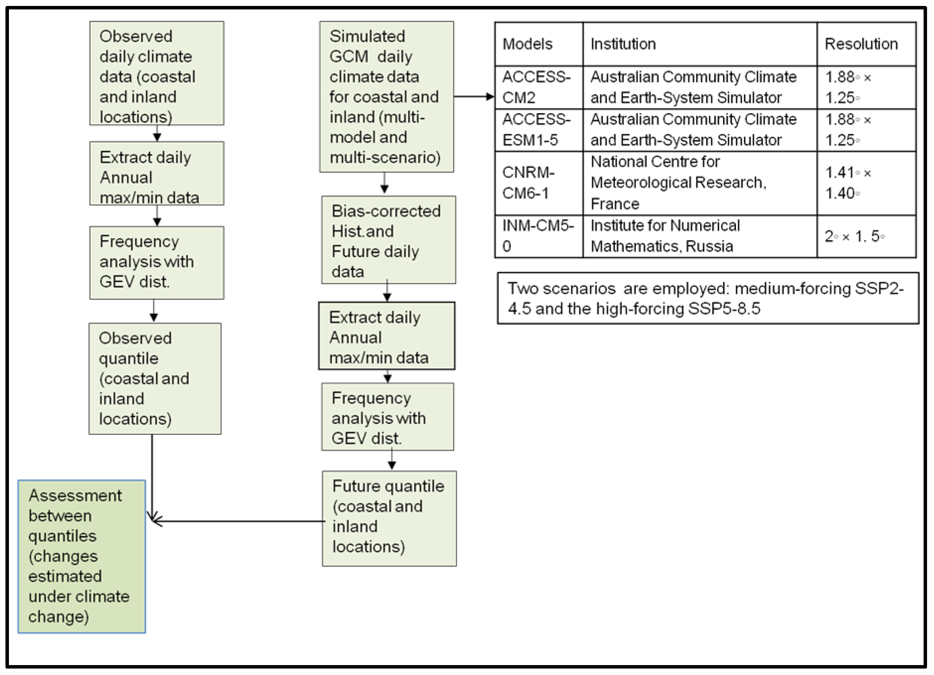
The overall analysis is illustrated in a flow chart in Figure 1.

Figure 1.
Proposed framework for evaluating climate extremes under climate change using a multi-model ensemble approach. The employed GCMs and scenarios are listed in the framework.
2.3. Observed and Simulated Data
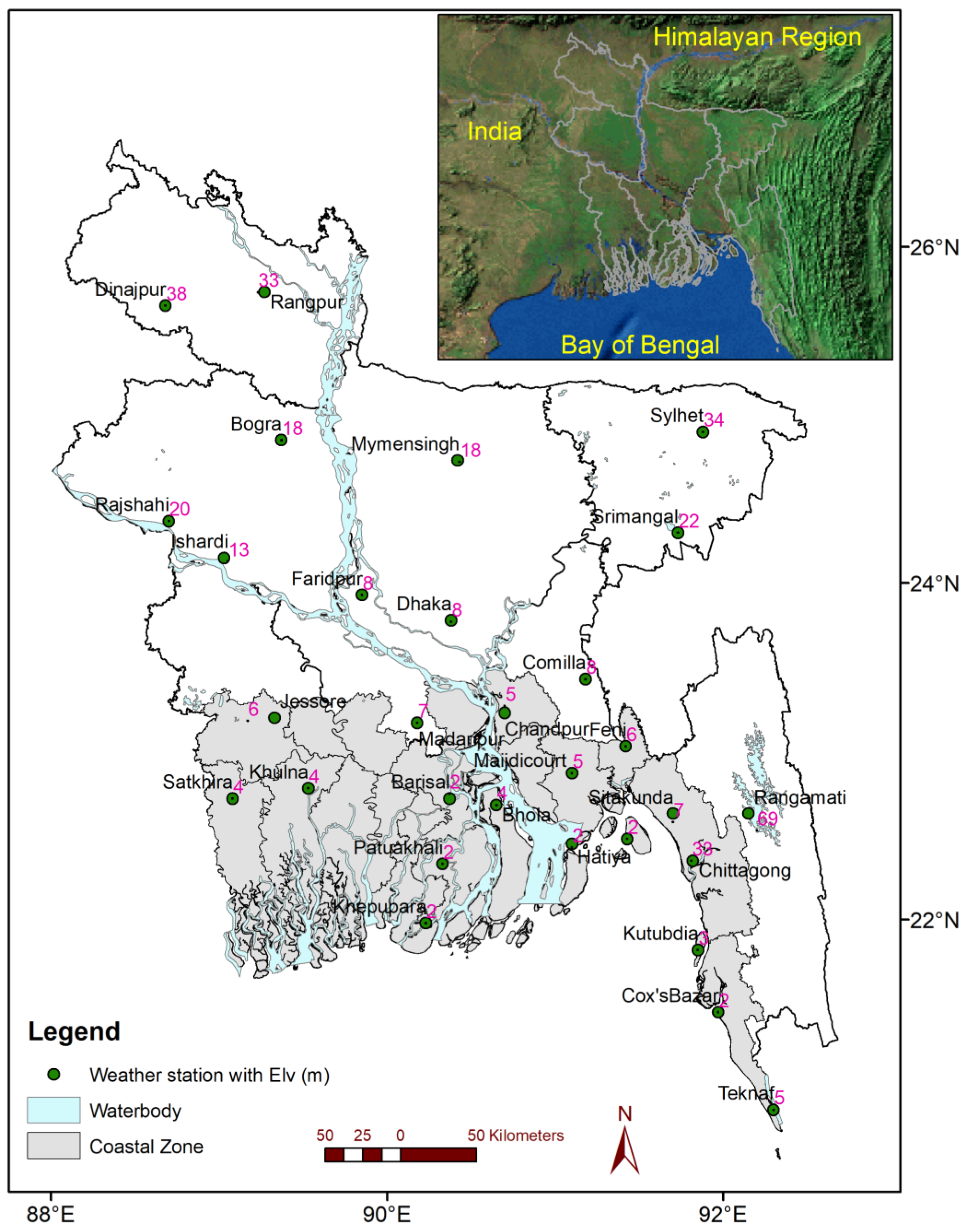
Observed daily rainfall, daily maximum and minimum temperature data of 35 stations were collected from the Bangladesh Meteorological Department (BMD). One of the major challenges with observational data is the missing data. Continuous rainfall records (<2% missing data) of more than 28 years (1986–2014) are available at only 30 stations. Thus, the data from 30 stations were considered in this study. The missing data in this case (<2% of the data) were replaced by the average values of three nearest neighboring stations. The locations of the considered stations are shown in Figure 2.
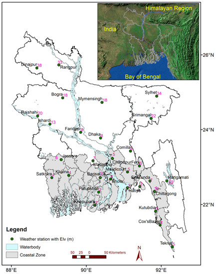
Figure 2.
Map of Bangladesh showing coastal (gray color) and inland regions (white color) with location of weather stations. The coastal zone is defined by the Bangladesh Government according to natural systems and events that govern its opportunities and vulnerabilities [76]. The elevation (m) associated with stations (number in pink color) are also indicated in the plot.
In Bangladesh, the coastal zone is defined by the Bangladeshi Government according to natural systems and events that govern its opportunities and vulnerabilities [76]. It includes factors such as tidal variations, soil salinity levels, surface or groundwater salinity and, cyclonic and storm surge risks. According to these processes, the coastal zone is made up of sixteen districts in the southern part of the country (out of sixty-four) [21]. The coastal locations are emphasized in the map. Out of 30 stations, 17 stations fall in this area. The remaining 13 are considered inland stations. Annual maximum (minimum) data were used to model extremes in this work. The series of annual maximum (rainfall of one-day duration and daily maximum temperature) and annual minimum (daily minimum temperature) were extracted for each station.
We obtain climate projections from the state-of-the-art CMIP6 framework. We use four GCMs in our analysis, which are listed in Figure 1. These climate models were selected based on the result of the work by [66]. These models came out as the top ranked GCMs in simulating Bangladesh observed climate.
Simulated data from four GCMs under two SSPs (medium-forcing SSP2-4.5 and the high-forcing SSP5-8.5) were obtained from the Earth System Grid Data Portal: https://esgf-node.llnl.gov/search/cmip6 (accessed on 5 October 2022). The medium and high-forcing scenarios SSP2-4.5 and SSP5-8.5 are selected for this work, which is deemed appropriate for covering the uncertainty of the estimate of future conditions of Bengal delta. The simulated daily rainfall, daily maximum and daily minimum temperature data were obtained for Bangladesh at 30 meteorological stations over the period 2021–2100. The data used in this study were already bias corrected. The performance of the bias-corrected data was evaluated by [32,33].
3. Results
3.1. Characteristics of Observed and Bias-Corrected Data
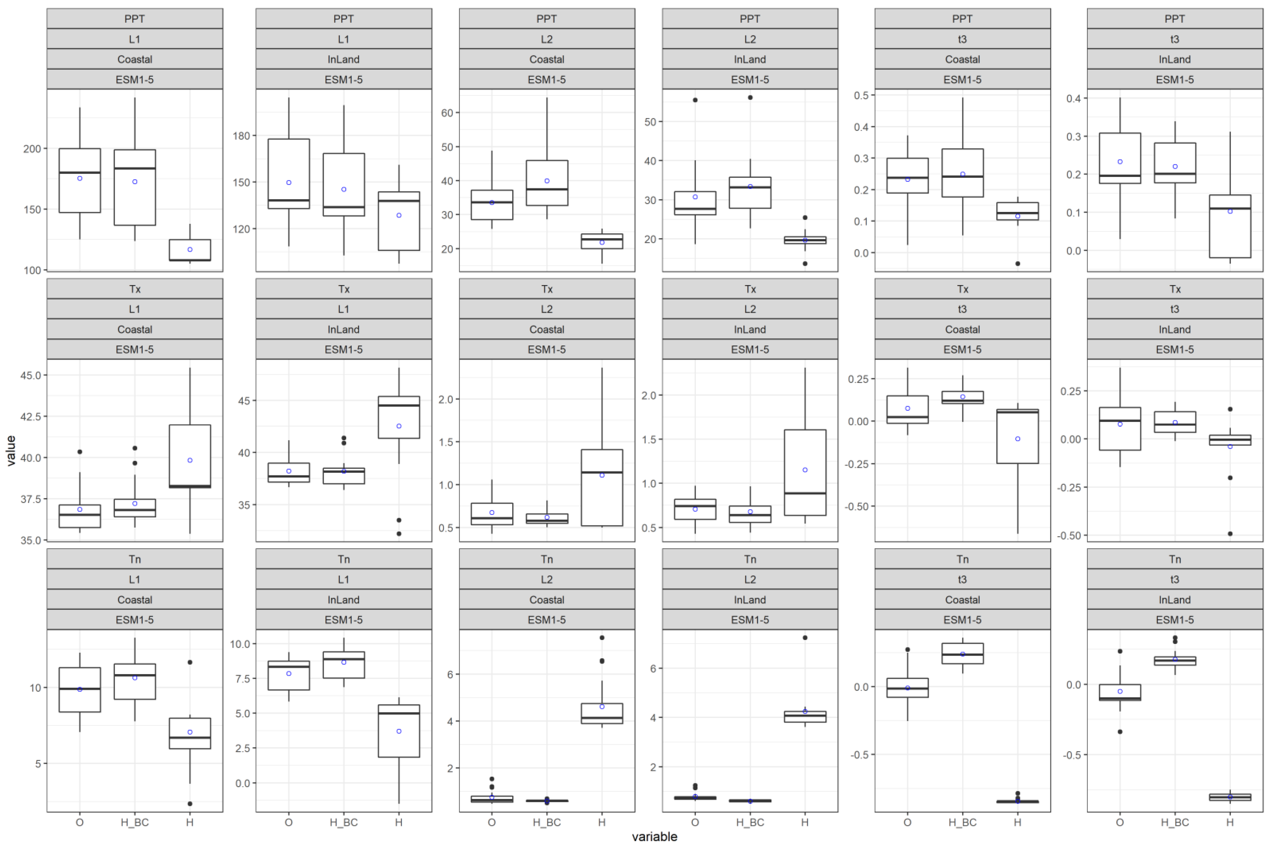
We analyzed three climate extremes—namely rainfall of 1-day duration (PPT), daily maximum temperature (Tx) and daily minimum temperature (Tn)—based on L-moments to understand the behavior of the datasets. The crucial L-moments: first L-moment second L-moment and L-skewness were estimated for both observed and simulated datasets. Figure 3 shows the estimated L-statistics in box plots for the present condition. The plots are also used to demonstrate the performance of the bias-corrected data in simulating L-statistics. The plots include the statistics derived from the observed data (specified as ‘O’); bias-corrected historical data (specified as ‘H_BC’) and simulated historical uncorrected data (specified as ‘H’). The assessment regarding inland and coast are separately shown in box plots. The title of each plot indicates the above attributes including the type of extremes assessed (PPT, Tx or Tn). Values from 13 stations are included in inland box plots while 17 stations are included in coastal box plots. The L-moment values are only displayed for ESM1-5 climate model for demonstration purpose. The average value (denoted as blue circle) is pointed out on each box plot so that an appraisal can be obtained.
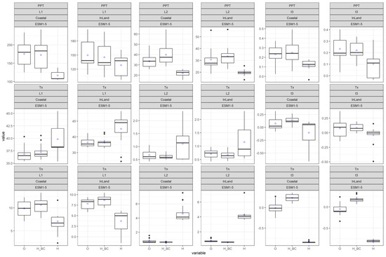
Figure 3.
Performance of bias-corrected data. Box plots of fitted L−moments (1st L−moment (L1), 2nd L−moment (L2) and L−skewness (t3)) at observed and simulated historic conditions ( data from GCM model, ESM1−5, is used for demonstration) for PPT, Tx and Tn for both coastal and inland region. ‘O’ represents estimate of L−moments based on observed data while ‘H_BC’ and ‘H’ represent L-moments estimate, respectively based on bias-corrected historical and uncorrected historical simulated data. The “blue circle” on each box plot represents the average value.
There is a considerable difference recognized between statistics of observed data and simulated historical uncorrected data. This is true for both the inland and coastal region. Quite a big margin of underestimation is noticed by the uncorrected PPT historical data of ESM1-5 model (see Figure 3: first row). With the bias-corrected data, the L-statistics present quite a similar average value to that of the observed data. The similar characteristic (average value of observed and bias-corrected data) is also noticed for Tx and Tn (Figure 3: second and third row). Overall, bias-corrected data mimic the observed data quite well. Hence, this is a significant enhancement. The analogous performance is recognized for other considered GCMs (Figures S1–S3) which have been included in the Supplementary File.
3.2. Examination of Parameters
Three climate extremes, PPT, Tx and Tn, were analyzed for coastal and inland locations. Annual maximum datasets of PPT and Tx and annual minimum datasets of Tn were fitted to GEV distribution. Three GEV parameters, specifically location, scale and shape, were estimated using the method of L-moments (see Equations (5)–(7)).
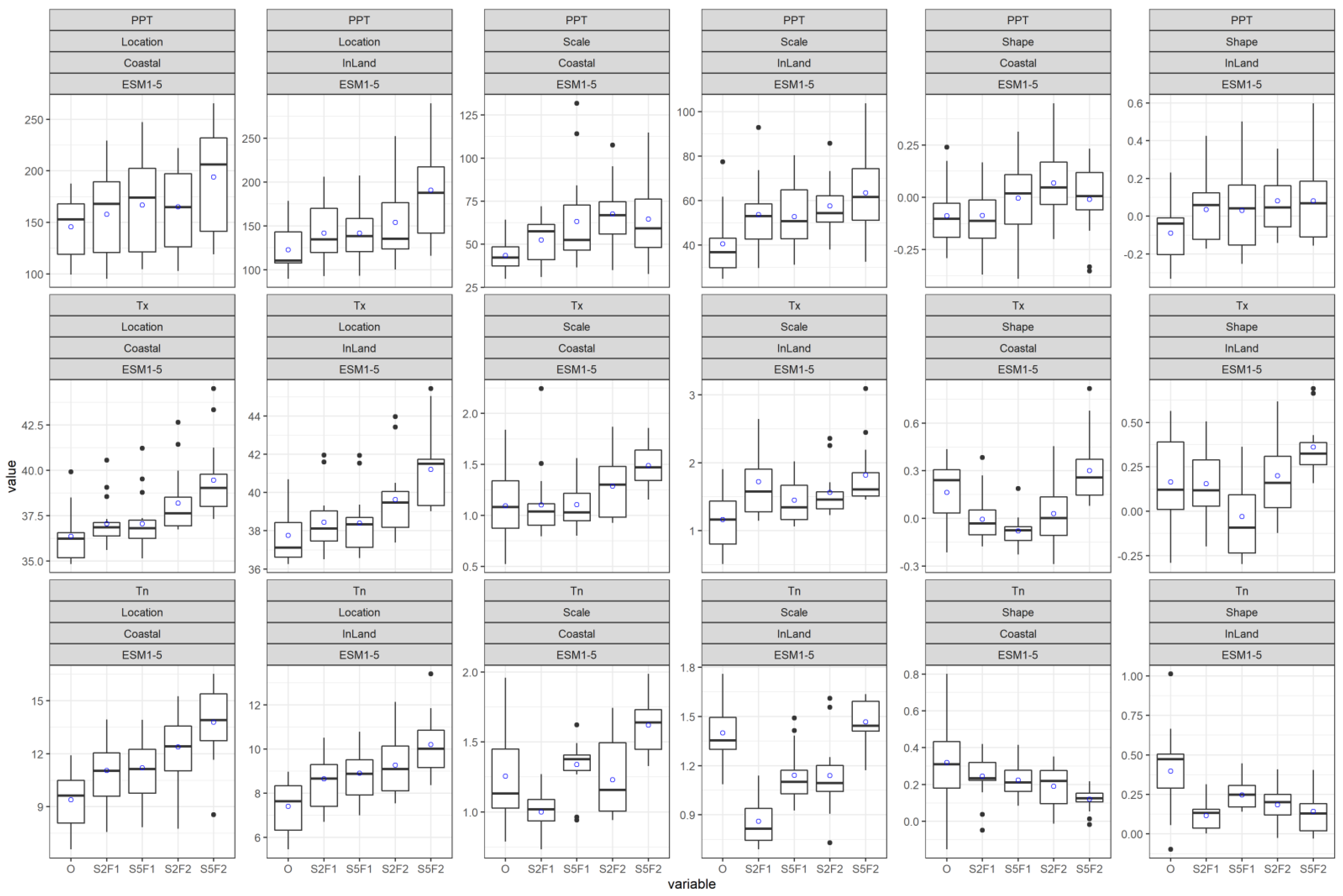
Figure 4 shows the parameter values in box plots for PPT, Tx and Tn. The assessment regarding inland and coast are separately shown in box plots. The title of each plot indicates the above attributes, including the type of extremes assessed (PPT, Tx or Tn). Values from 13 stations are included in inland box plots, while 17 stations are included in coastal box plots. The plots comprise parameters derived from observed and simulated bias-corrected future data. The simulated data include near future (F1:2021–2060) and far future (F2: 2061–2100) under two SSPs: 245 and 585 derived from the considered GCM models. The parameter values are only displayed for the ESM1-5 climate model for demonstrative purposes. The average value (denoted as blue circle) is pointed out on each box plot so that an appraisal can be obtained.
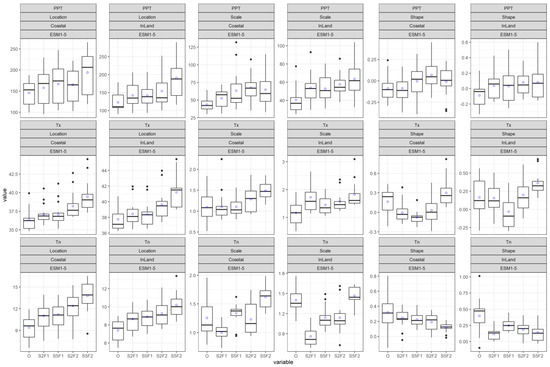
Figure 4.
Box plots of fitted GEV parameters (Location, Scale and Shape) at observed (o) and future conditions (only data from GCM model, ESM1-5, is used for demonstration) for PPT, Tx and Tn for both coastal and inland region. Future scenarios were represented by ‘S245F1’, ‘S585F1’, ‘S245F2’ and ‘S585F2’, where S245 and S585, respectively, designate SSP245 and SSP585, and F1 and F2, respectively designate the near (2021–2060) and far future (2061–2100). The “blue circle” on each box plot represents the average value.
Regarding location parameters for the observed case, the mean PPT value is considerably higher (145 > 122) in the coastal region than inland (see first and second plot of row 1 of Figure 4). In case of temperature extremes, the contrasting behavior is noticed. A higher Tx value is observed inland compared to the coastal locations (37.7 > 36.3), while for Tn the opposite is noted: the inland value is lower than coastal value (7.4 < 9.4).
The behavior of the location parameter under climate change for all the extremes gives similar characteristics (see all plots of columns 1 and 2 of Figure 4): the higher-emission scenario presents a greater value than that of the medium emission scenario. So does the far future time horizon, which gives a higher value than that of the near future. The attribute holds true for all the selected GCMs. This points out that the location of the distribution shifts rightwards under the impact of climate change.
Regarding scale parameters for the observed case, the average PPT value is higher in coastal regions than inland, which translates to a higher dispersion in coastal datasets. The value of the shape parameter in both cases is quite similar (under zero, i.e., unbounded) which suggests the skewness of both datasets is in the same range. The scale and shape parameters of Tx and Tn are also in the same range for both coastal and inland locations. The shape parameter is upper bounded in both cases for Tx and Tn, which means the skewness is low compared to rainfall value, which is expected.
A similar discernible pattern (such as a location parameter) under climate change is absent for scale and shape parameters (except for PPT, where a moderately increasing trend is noted for scale parameter). In certain situations, the average scale and shape parameters are lower in the far future than in the near future, and vice versa. From this, it is inferred that there would be no orderly changes in the shape of frequency in the future. From this, it can also be concluded that a substantial amount of uncertainty prevails in the future extremes.
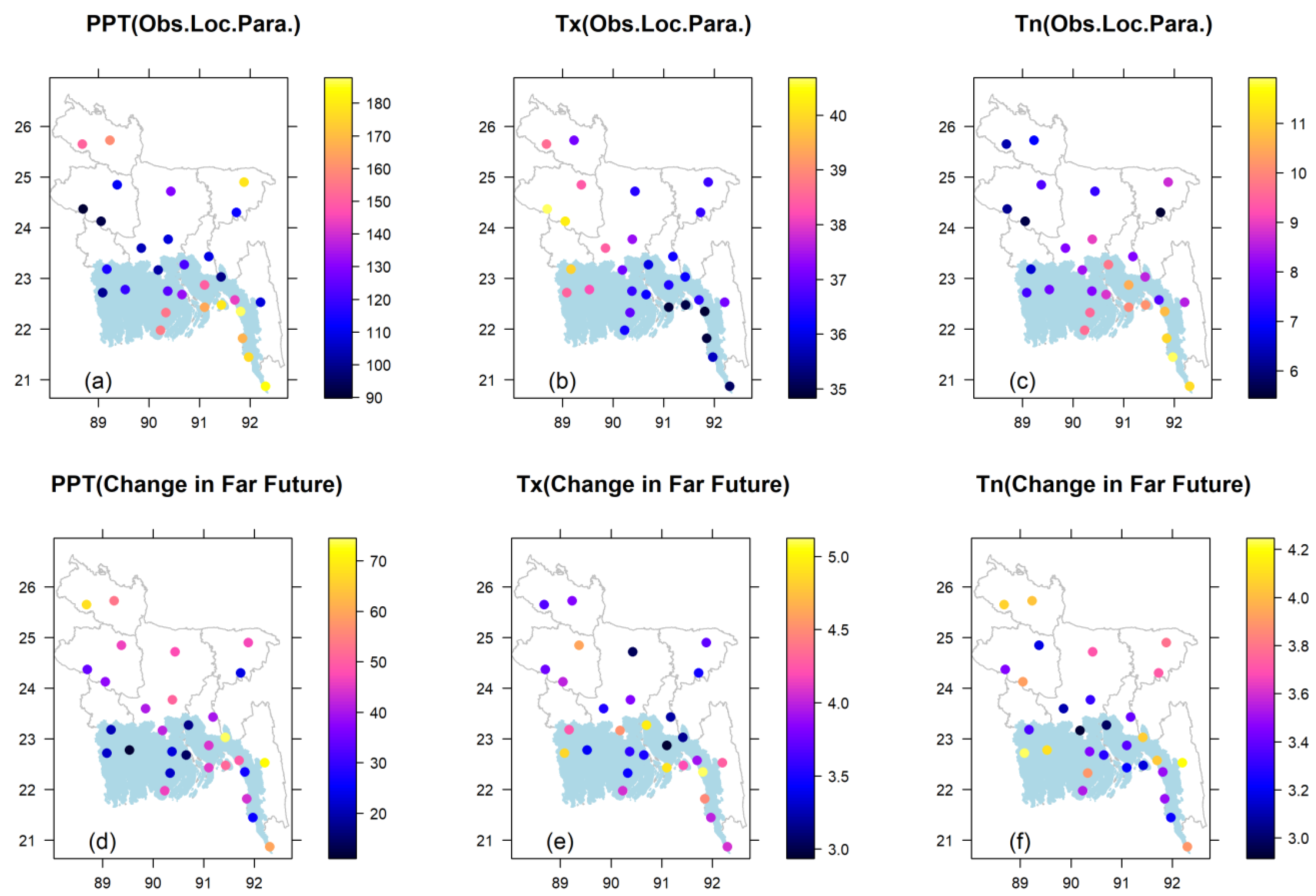
Since the location parameter has a clear trend (which also influences the extreme estimate to a great extent), the spatial distribution of the parameter has been displayed over the study region. Maps for the observed case and maps for the changes in values under climate change are shown in Figure 5. The change is assessed with respect to the observed value. Only the changes with reference to the scenario: SSP585 (far future) are used.
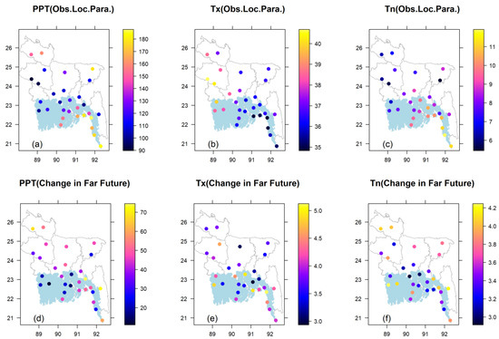
Figure 5.
Spatial distribution of location parameters based on observed data, (a) PPT, (b) Tx, and (c) Tn and their changes in location for (d) PPT, (e) Tx, and (f) Tn under climate change with scenario SSP585 in the far future.
The observed parameter values for PPT are highest along the coast, extreme north, and north-east (inland area) near the Himalayan regions (Figure 5a). The lowest values are generally observed in the west side, which mainly falls in the inland area. Change values are site dependent, and different values are recognized across the study area. The highest positive changes can generally be found along the coast (south-east) and north-middle part of the country (Figure 5d). The lowest positive changes are noticed in the west side.
The spatial pattern of observed Tx is quite opposite to PPT. The highest values are generally observed in the west side, which mainly falls in the inland area (Figure 5b). The lowest values are found along the coast and eastern half of the country. The highest positive (increased) changes are recognized in the south-east along the coast (Figure 5e). Contrasting spatial behavior is observed for Tn with reference to Tx. The lowest observed values are noticed in the west, but they are moderated along the coast in the south (Figure 5c). The highest positive changes are found in the middle–northern part of the country (Figure 5f).
Hence, climate change is predicted to increase the location parameters in all extreme cases in both coastal and inland locations—rainfall amount should progress to higher levels and extreme temperatures should shift to warmer values.
3.3. Assessment of Extreme Quantile
With the estimated parameters, extremes in terms of return levels were calculated. The analysis reported here for the 50-year return level (PPT50, Tx50, and Tn50) represents a medium-high quantile value. The changes of extreme values for those cases under climate change were also evaluated.
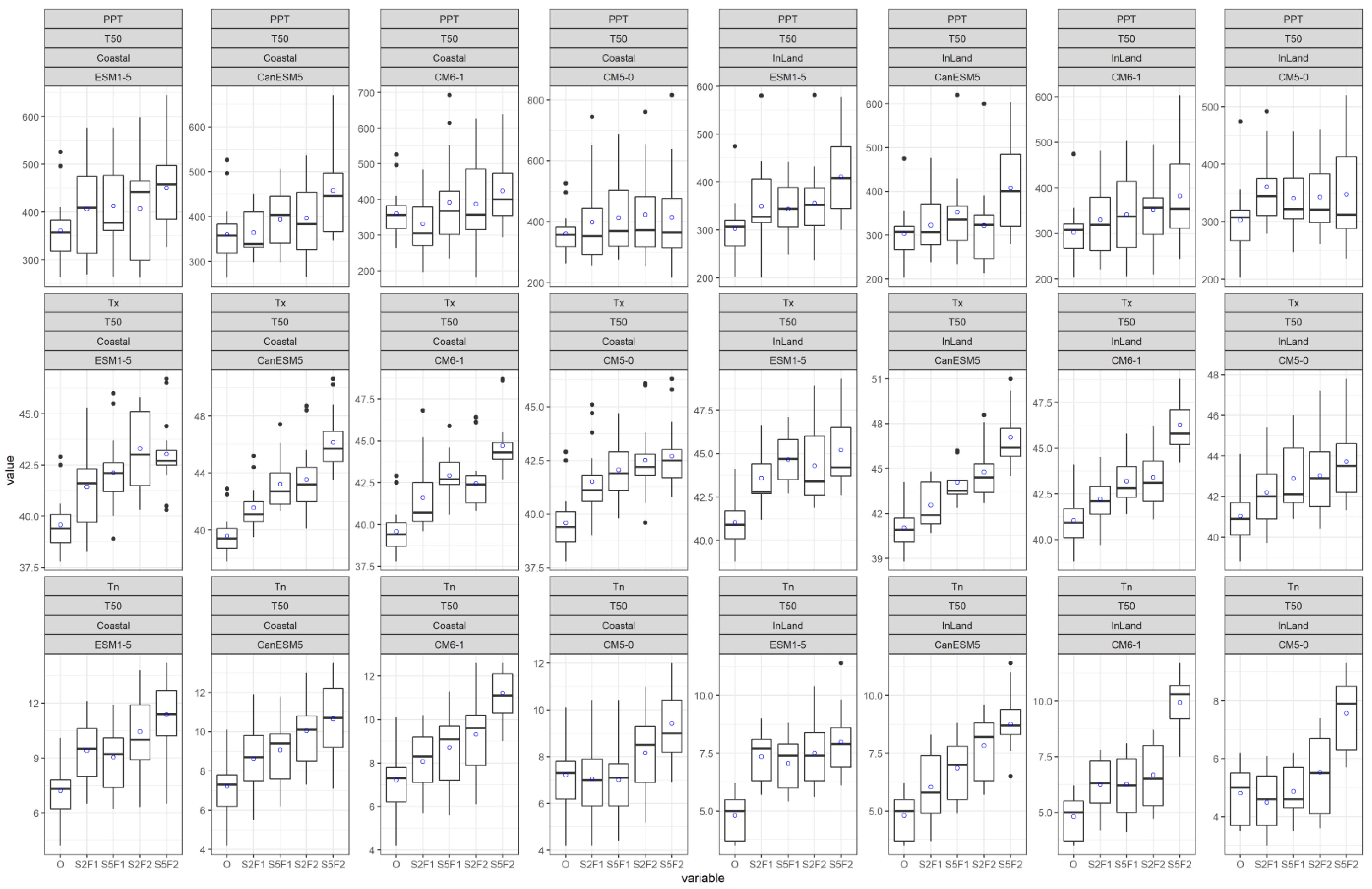
Figure 6 shows the quantile values in box plots for all the GCMs considered in this study. First row of Figure 6 shows the quantile values for PPT, while the second and third row, respectively, show the quantile values for Tx and Tn. Inland and coastal values are shown separately in the figure. Estimated quantiles are displayed for the observed data, as well as for simulated data derived from all the considered GCMs. The mean values for observed, as well as future climate (for both scenarios), are summarized for coastal and inland locations in Table 1.
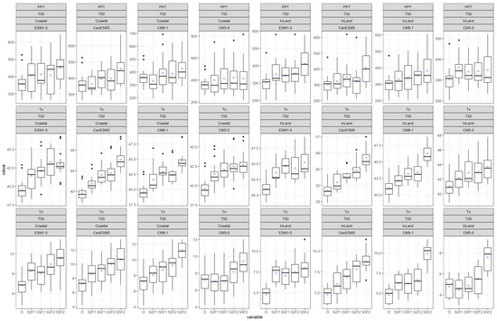
Figure 6.
Box plots of 50-year return level at observed (o) and future conditions (simulations from 4 GCMs) for PPT, Tx and Tn. Future scenarios were represented by ‘S245F1’, ‘S585F1’, ‘S245F2’ and ‘S585F2’ where S245 and S585, respectively, designate SSP245 and SSP585, and F1 and F2, respectively designate future time horizon 2021–2060 and 2061–2100. The “blue circle” on each box plot represents the average value.

Table 1.
Coastal and inland average estimate of climate extremes at present and under climate change with different scenarios in two future time horizons.
The observed mean value of PPT50 is considerably higher (about 20%) in coastal regions than in inland areas. In case of temperature extremes, the contrasting behavior is observed for Tx and Tn. In case of Tx50, a higher value is noticed for inland than coastal locations (the difference is about 1.4 °C), and the opposite is observed for Tn50 (the difference is about 2.4 °C).
Under climate change, the quantile values increase for all the extremes. A greater value is identified in the far future than in the near future. The larger value is also found in the higher-emission scenario compared to the medium-emission scenario. However, the differences between coastal and inland estimates vary under climate change. For rainfall, it is expected to increase in PPT50 by 76 mm (22%) for coastal regions, while for inland locations, the value is about 85 mm (28%) under SSP585 in the far future. This suggests that the difference in PPT50 value between coastal and inland is reduced under climate change. Nonetheless, the inland estimate under climate change is barely able to exceed the observed coastal estimate.
Regarding coastal extreme temperature, the SSP585 suggests an increase in Tx50 of 4.5 °C by the end of the century. With Tn50, the value is 3.5 °C. Inland, the scenario indicates an increase in Tx50 of 4.6 °C, which is quite similar to that of the coast. With Tn50, the increase is about 3.8 °C. This implies that the difference in Tx50 under climate change is quite similar to the observed difference between coastal and inland locations (1.5 °C compared to observed 1.4 °C). However, for Tn50, the difference is reduced a little (2.1 °C compared to the observed difference of 2.4 °C) under climate change.
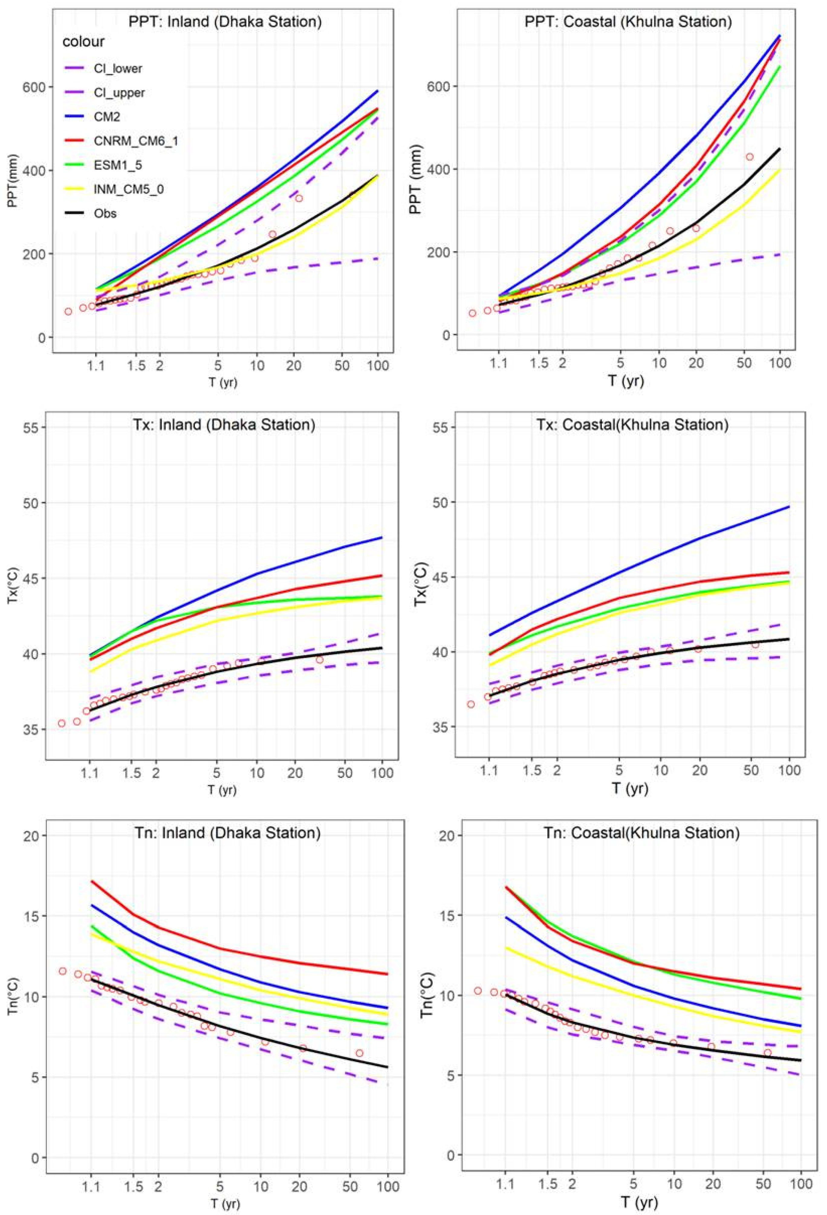
Considerable uncertainty is present in estimating quantile values which have been shown by the box plots (see Figure 6). Further, two stations were selected, namely Dhaka (inland) and Khulna (coastal), to demonstrate the uncertainty in the probability plots (return period value in terms of years) at an individual station. Figure 7 shows the plots for PPT, Tx and Tn for observed and future conditions. Projections from the scenario SSP585 in the far future were used to display the plots. The probability plots using observed data (solid black line) and the associated 95% confidence intervals, CI, (dotted lines) are also shown. The CIs were constructed based on a bootstrapping method. They can be represented as curves due to climate variability.
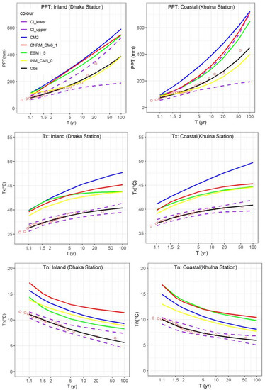
Figure 7.
Examination of probability plots of climate extremes (PPT, Tx and Tn) at observed and future conditions (4 GCMs under SSP585 in the far future) for the selected coastal and inland stations. The y axis represents return period (T) in years.
In most instances, the CIs were outstripped by the curves derived from the future simulated data. That implies that the impact of climate change is significant, and it can change the frequency of climate extremes for both coastal and inland regions of Bengal delta. It also shows that different quantiles were obtained by different GCMs at different locations.
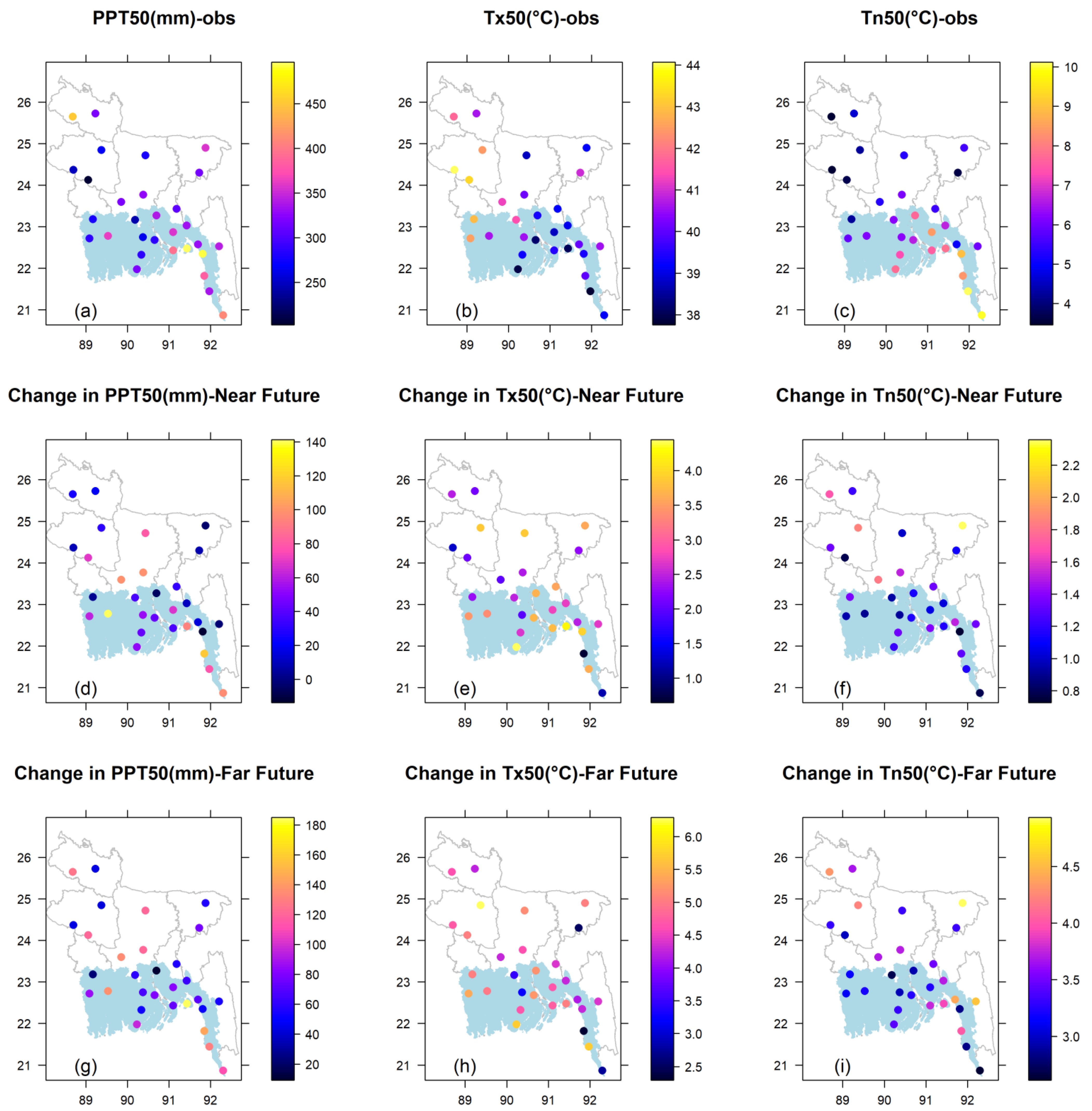
We also constructed maps for 50-year quantile values for observed cases (Figure 8a–c) and maps of change values (difference between future and observed estimate) (Figure 8d–i) under climate change to reveal the spatial behavior of extreme quantiles. The change values of extremes are displayed for the scenario SSP585 in the near and far future.
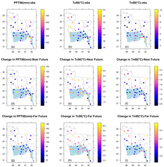
Figure 8.
Spatial distribution of 50-year quantile based on observed data (a) PPT (mm); (b) Tx (°C) and (c) Tn (°C) and their changes under high emission scenario (SSP585) in the near future: (d) change in PPT (mm); (e) change in Tx (°C); and in the far future: (f) change in Tn (°C) and in the far future; (g) change in PPT (mm); (h) change in Tx (°C); (i) change in Tn (°C).
Since the location parameter dominates the estimate to a great extent, the spatial characteristics of observed estimates are quite similar to that of the location parameter. However, in some sites, they behave quite differently, and that is due to the influence of scale and shape parameters of that site. The observed values of PPT50 are the highest along the coast and the extreme north (inland area) near the Himalayan regions (Figure 8a). The lowest values are generally observed in the west side, which mainly falls in the inland area. The change values under climate change are different across the country. Highest increase (positive changes) values of PPT50 can be found along the extreme southern coast and northern-middle part of the country (Figure 8d,g). The lowest positive changes generally are observed in the west and eastern side.
In case of temperature extremes, contrasting behavior is noted for Tx50 and Tn50. The highest observed values are generally found in the west side, which mainly falls in the inland area. The lowest values are prominent along the coast and eastern half of the country (Figure 8b). Change values are different in different locations; however, the highest positive changes are noticed in the southern coastal locations and middle-western inland area (Figure 8e,h). The spatial pattern of observed Tn50 is quite opposite to Tx50. The lowest observed estimates are predominantly found in the western side, but medium to high values are identified in the south along the coast (Figure 8c). The change values are quite uniform compared to Tx, but the highest positive changes are observed generally in inland area (Figure 8f,i). Quite a similar pattern of changes is obtained for the near and far future; however, the greatest changes are shown in the far future.
4. Discussion
The purpose of this work is to compare the effects of climate change on climate extremes between coastal and inland locations based on an ensemble of GCMs derived from CMIP6.
Since very often, the generated data from GCMs do not satisfactorily simulate the observed data at the local scale, bias correction is often considered. This is normally carried out to reduce the errors. In this study, the bias-corrected data (evaluated based on summary L-moments) reduced the error quite appropriately (see Figures S1–S3 in the Supplementary File). The observed and bias-corrected data show similar characteristics which indicate its effectiveness. This is in agreement with the past studies in this region [32,33].
We employed a GEV-based frequency model to analyze extremes at present and under climate change conditions. In regard to GEV parameters, the location is the only parameter that increases linearly under climate change for all the extremes in both regions. This suggests a uniform repositioning of the location parameter to the right for the extreme tail of the GEV distribution. There are no such considerable changes in scale and shape parameters. The result compliments the effective non-stationary analysis, where location is always used as the time-dependent variable [77,78].
The noteworthy increase in location parameter (Figure 4) reflects the overall changes in the return period values (See Figure 6). The extremes increase appreciably under climate change throughout the country (See Figure 8). This reveals that extreme rainfall and temperatures have the tendency to increase markedly by the end of this century, which is in line with the previous studies worldwide [9,10,34,45,53,54,55,79,80,81]
The spatial behavior of observed climate extremes is quite similar to that of location parameters. This happens because the location parameter dictates the quantile to a great degree, especially when the return period is low to medium [52,82]. Rainfall extremes in both coastal and inland locations are expected to amplify noticeably, which is generally in accord with the previous studies in the study region [21,22]. However, a slightly higher rate of increase of extreme rainfall is expected in inland locations, which is in agreement with the findings in [21]. Thus, the difference of estimate under climate change is reduced a little compared to the observed difference. Nonetheless, the inland estimate under climate change is barely able to exceed the observed coastal estimate. As a result, it can be said that the coastal region is expected to be more vulnerable to heavy storm and subsequent severe flooding. In regard to temperature extremes, both coastal and inland locations are expected to increase appreciably, which is in line with the previous studies [21,22,27], but the inland region displayed a slight increase in Tx, which is quite in agreement with the outcome in Bangladesh [28,83]. With Tn, the increase rate is higher in inland locations than in the coastal region. The amplification of Tx, in particular, in the north-western inland area is of great concern, because desertification is already on the rise [30,84]. With further increase, the region is vulnerable to severe drought in the future.
It is also recognized that warming rates of Tx (in both regions) exceed that of Tn (see Table 1) which is in line with the outcome for subtropical and tropical territories [10], including Bangladesh [29].
Overall, the coastal area is expected to be more vulnerable to flooding, while the inland area to drought in the Bengal delta region. Even though the inland area is prone to drought, the extreme rainfall is expected to increase there. Changes in dynamic and thermodynamic activity can explain a significant increase in the maximum one-day rainfall during warmer circumstances [85,86].
The extreme estimates under climate change, based on which outcomes are drawn, are subject to uncertainty. Using four GCMs and two SSPs suitable for Bangladesh, we satisfactorily envelop the larger degree of uncertainty that has been displayed in several assessments (See Figure 4, Figure 6 and Figure 7). There is visible inter-model uncertainty in the projected extremes, as indicated in Figure 7. This uncertainty should be taken into account when estimation is sought; for example, for risk management of floods and drought. The intra-model uncertainty (uncertainty within the model) is also an issue with the climate change impact analysis. To accurately assess the uncertainty, it is envisaged to carry out the intra-model uncertainty by including a member ensemble to a particular GCM. Thus, further investigation is required in this direction.
Topography is also considered an important factor inducing biases in the simulated datasets [87,88]. In high elevation areas, the GCM is likely to introduce bias, since it assumes a smoother and lower topography than is actually the case [89]. The considered study area is relatively a less complex topography (about 80% plain land), and hilly regions are in the northeast and southeast of the inland areas [90]. A similar degree of biases is recognized (in simulating summary L-statistics) in coastal and inland regions (see Figure 3 and related figures (Figures S1–S3) in the Supplementary File). However, a detailed examination in the hilly regions is required to understand the fully fledged topographical effect on GCMs.
The findings of our study have noteworthy policy implications for the delta region. With a substantial rise in extreme temperature on the cards, sustained drought may surface in the northern and western territories. Drought-tolerant agricultural cultivars and optimal use of surface water resources may be necessary to adapt to the drying circumstances. Additionally, with the rise in extreme temperatures, the saline water intrusion in the southern region might be exacerbated under climate change [29], which requires effective water resources management. With the expectation of increase in extreme rainfall over the coastal regions, the risk of severe floods and landslides might be aggravated, which leads to a need for sustainable flood risk management.
5. Conclusions
This work compares the effect of climate change on climate extremes between coastal and inland locations in the Bengal delta region. The multi-model ensemble method was employed to examine the impact in two future time horizons: 2021-2060 and 2061–2100. The GEV-based frequency analysis was applied to study the climate extremes at present and under climate change conditions.
The conclusions obtained from the study are summarized below:
- The location parameter of GEV is expected to increase linearly under climate change in rainfall and temperature extremes for both coastal and inland regions. Changes in location suggest a uniform repositioning for the extreme tail of the GEV. There are no such substantial changes in scale and shape parameters.
- The coast and inland both are expected to amplify the extreme rainfall considerably. The rate of increase is slightly higher in inland locations under climate change; nonetheless, the inland estimate by the end of the century is barely able to exceed the observed coastal estimate.
- In regard to temperature extremes, both coastal and inland locations are expected to increase appreciably under climate change. With Tx, the rate of increase is almost similar; however, with Tn, the increase rate is slightly higher in inland locations than in the coastal region. The coastal and inland average change in Tx50 by the end of this century is, respectively, 4.5 and 4.6 °C in the SSP585 experiment, compared to the corresponding changes of 3.5 and 3.8 °C in Tn50. The warming rates of Tx surpass those of Tn.
- The coastal area is expected to be more vulnerable to flooding, while the inland is more vulnerable to drought under climate change in the Bengal delta region.
The present study considers four GCMs to complete the assessment. Further investigation is needed to assess the uncertainty in full scale (inter and intra-variability) by including more GCMs and a member ensemble in a particular GCM model. The findings of our work have key scientific and practical implications for highly vulnerable regions, such as the Bengal delta, in terms of water resource management; agricultural arrangement; and flood and drought deterrence. The study is expected to assist decision makers with developing ways to offset the effects of climate extremes in coastal and inland locations.
Supplementary Materials
The following supporting information can be downloaded at: https://www.mdpi.com/article/10.3390/atmos13111747/s1, Figure S1: Performance of bias-corrected data for the GCM model: CanESM5, Figure S2: Performance of bias-corrected data for the GCM model: CNRM-CM6-1, Figure S3: Performance of bias-corrected data for the GCM model: INM-CM5-0.
Author Contributions
Conceptualization, S.D.; methodology, S.D.; software, S.D.; validation, S.D.; formal analysis, S.D.; investigation, S.D.; resources, S.D.; data curation, M.K.; writing—original draft preparation, S.D., M.K. and A.R.M.T.I.; writing—review and editing, S.D., A.K. and D.Z.; visualization, S.D.; supervision, S.D.; project administration, S.D.; funding acquisition, S.D. All authors have read and agreed to the published version of the manuscript.
Funding
This research was funded by Nanjing University of Information Science and Technology, grant number 2243141501015 of the first author.
Institutional Review Board Statement
Not applicable.
Informed Consent Statement
Not applicable.
Data Availability Statement
The observed daily rainfall and temperature data were obtained from the Bangladesh Meteorological Department: http://live4.bmd.gov.bd/ (accessed on 5 October 2022). The observed data are available on request from the corresponding author. Simulated data from four GCMs under two SSPs (medium-forcing SSP2-4.5 and the high-forcing SSP5-8.5) were obtained from the Earth System Grid Data Portal: https://esgf-node.llnl.gov/search/cmip6 (accessed on 5 October 2022).
Acknowledgments
The authors thank the three anonymous reviewers for their critical comments, which helped improve the quality of the manuscript.
Conflicts of Interest
The authors declare no conflict of interest.
References
- IPCC. Summary for Policymakers. In Global Warming of 1.5 °C.; An IPCC Special Report on the impacts of global warming of 1.5 °C above pre-industrial levels and related global greenhouse gas emission pathways, in the context of strengthening the global response to; World Meteorological Organization: Geneva, Switzerland, 2018. [Google Scholar]
- IPCC. Summary for Policymakers in Climate Change 2013: The Physical Science Basis, Contribution of Working Group I to the Fifth Assessment Report of the Intergovernmental Panel on Climate Change; Stocker, T.F., Qin, D., Plattner, G., Tignor, M., Allen, S.K., Boschung, Eds.; Cambridge University Press: Cambridge, NY, USA, 2013. [Google Scholar]
- Palazzi, E.; von Hardenberg, J.; Terzago, S.; Provenzale, A. Precipitation in the Karakoram-Himalaya: A CMIP5 view. Clim. Dyn. 2015, 45, 21–45. [Google Scholar] [CrossRef]
- Alexander, L.V.; Zhang, X.; Peterson, T.C.; Caesar, J.; Gleason, B.; Tank, A.M.G.K.; Haylock, M.; Collins, D.; Trewin, B.; Rahimzadeh, F.; et al. Global observed changes in daily climate extremes of temperature and precipitation. J. Geophys. Res. Atmos. 2006, 111, 1042–1063. [Google Scholar] [CrossRef]
- Easterling, D.R.; Evans, J.L.; Groisman, P.Y.; Karl, T.R.; Kunkel, K.E.; Ambenje, P. Observed variability and trends in extreme climate events: A brief review. Bull. Am. Meteorol. Soc. 2000, 81, 417–425. [Google Scholar] [CrossRef]
- Trenberth, K.E.; Jones, P.D.; Ambenje, P.; Bojariu, R.; Easterling, D.; Klein Tank, A.; Parker, D.; Rahimzadeh, F.; Renwick, J.A.; Rusticucci, M. Observations. Surface and atmospheric climate change. In Climate Change 2007: The Physical Science Basis. Contribution of Working Group 1 to the 4th Assessment Report of the Intergovernmental Panel on Climate Change; Cambridge University Press: Geneva, Switzerland, 2007; Chapter 3. [Google Scholar]
- Shaby, B.A.; Reich, B.J. Bayesian spatial extreme value analysis to assess the changing risk of concurrent high temperatures across large portions of European cropland. Environmetrics 2012, 23, 638–648. [Google Scholar] [CrossRef]
- Papalexiou, S.M.; Montanari, A. Global and Regional Increase of Precipitation Extremes Under Global Warming. Water Resour. Res. 2019, 55, 4901–4914. [Google Scholar] [CrossRef]
- Fowler, H.J.; Ali, H.; Allan, R.P.; Ban, N.; Barbero, R.; Berg, P.; Blenkinsop, S.; Cabi, N.S.; Chan, S.; Dale, M.; et al. Towards advancing scientific knowledge of climate change impacts on short-duration rainfall extremes. Philos. Trans. R. Soc. A Math. Phys. Eng. Sci. 2021, 379, 20190542. [Google Scholar] [CrossRef]
- Kharin, V.V.; Zwiers, F.W.; Zhang, X.; Wehner, M. Changes in temperature and precipitation extremes in the CMIP5 ensemble. Clim. chang. 2013, 119, 345–357. [Google Scholar] [CrossRef]
- Tebaldi, C.; Hayhoe, K.; Arblaster, J.M.; Meehl, G.A. Going to the extremes: An intercomparison of model-simulated historical and future changes in extreme events. Clim. chang. 2006, 79, 185–211. [Google Scholar] [CrossRef]
- Kharin, V.V.; Zwiers, F.W.; Zhang, X.; Hegerl, G.C. Changes in temperature and precipitation extremes in the IPCC ensemble of global coupled model simulations. J. Clim. 2007, 20, 1419–1444. [Google Scholar] [CrossRef]
- Frías, M.D.; Mínguez, R.; Gutiérrez, J.M.; Méndez, F.J. Future regional projections of extreme temperatures in Europe: A nonstationary seasonal approach. Clim. chang. 2012, 113, 371–392. [Google Scholar] [CrossRef]
- Tang, B.; Hu, W.; Duan, A. Future projection of extreme precipitation indices over the Indochina Peninsula and South China in CMIP6 models. J. Clim. 2021, 34, 8793–8811. [Google Scholar] [CrossRef]
- Das, S.; Millington, N.; Simonovic, S.P. Distribution choice for the assessment of design rainfall for the city of London (Ontario, Canada) under climate change. Can. J. Civ. Eng. 2013, 40, 121–129. [Google Scholar] [CrossRef]
- Losada, I.J.; Toimil, A.; Muñoz, A.; Garcia-Fletcher, A.P.; Diaz-Simal, P. A planning strategy for the adaptation of coastal areas to climate change: The Spanish case. Ocean Coast. Manag. 2019, 182, 104983. [Google Scholar] [CrossRef]
- Taherkhani, M.; Vitousek, S.; Barnard, P.L.; Frazer, N.; Anderson, T.R.; Fletcher, C.H. Sea-level rise exponentially increases coastal flood frequency. Sci. Rep. 2020, 10, 1–17. [Google Scholar] [CrossRef] [PubMed]
- Zhang, Y.; Wang, Y.; Chen, Y.; Liang, F.; Liu, H. Assessment of future flash flood inundations in coastal regions under climate change scenarios—A case study of Hadahe River basin in northeastern China. Sci. Total Environ. 2019, 693, 133550. [Google Scholar] [CrossRef]
- Abiodun, B.J.; Adegoke, J.; Abatan, A.A.; Ibe, C.A.; Egbebiyi, T.S.; Engelbrecht, F.; Pinto, I. Potential impacts of climate change on extreme precipitation over four African coastal cities. Clim. Change 2017, 143, 399–413. [Google Scholar] [CrossRef]
- Karbassi, A.R.; Maghrebi, M.; Lak, R.; Noori, R.; Sadrinasab, M. Application of sediment cores in reconstruction of long-term temperature and metal contents at the northern region of the Persian Gulf. Desert 2019, 24, 109–118. [Google Scholar]
- Abdullah, A.Y.M.; Bhuian, M.H.; Kiselev, G.; Dewan, A.; Hasan, Q.K.; Rafiuddin, M. Extreme temperature and rainfall events in Bangladesh: A comparison between coastal and inland areas. Int. J. Climatol. 2020, 42, 3253–3273. [Google Scholar] [CrossRef]
- Hasan, M.A.; Islam, A.K.M.S.; Akanda, A.S. Climate projections and extremes in dynamically downscaled CMIP5 model outputs over the Bengal delta: A quartile based bias-correction approach with new gridded data. Clim. Dyn. 2018, 51, 2169–2190. [Google Scholar] [CrossRef]
- Mirza, M.M.Q. Climate change, flooding in South Asia and implications. Reg. Environ. chang. 2011, 11, 95–107. [Google Scholar] [CrossRef]
- Sönke, K.; Eckstein, D.; Dorsch, L.; Fischer, L. Global Climate Risk Index 2016: Who Suffers Most from Extreme Weather Events? Weather-Related Loss Events in 2014 and 1995 to 2014; Germanwatch e.V.: Berlin, Germany, 2015; ISBN 9783943704044. [Google Scholar]
- Kamruzzaman, M.; Jang, M.W.; Cho, J.; Hwang, S. Future changes in precipitation and drought characteristics over Bangladesh under CMIP5 climatological projections. Water 2019, 11, 2219. [Google Scholar] [CrossRef]
- Sarker, M.A.R.; Alam, K.; Gow, J. Exploring the relationship between climate change and rice yield in Bangladesh: An analysis of time series data. Agric. Syst. 2012, 112, 11–16. [Google Scholar] [CrossRef]
- Khan, M.J.U.; Islam, A.K.M.S.; Das, M.K.; Mohammed, K.; Bala, S.K.; Islam, G.M.T. Observed trends in climate extremes over Bangladesh from 1981 to 2010. Clim. Res. 2019, 77, 45–61. [Google Scholar] [CrossRef]
- Shahid, S.; Wang, X.J.; Harun, S.B.; Shamsudin, S.B.; Ismail, T.; Minhans, A. Climate variability and changes in the major cities of Bangladesh: Observations, possible impacts and adaptation. Reg. Environ. chang. 2016, 16, 459–471. [Google Scholar] [CrossRef]
- Mallick, J.; Islam, A.R.M.T.; Ghose, B.; Islam, H.M.T.; Rana, Y.; Hu, Z.; Bhat, S.A.; Pal, S.C.; Ismail, Z. Bin Spatiotemporal trends of temperature extremes in Bangladesh under changing climate using multi-statistical techniques. Theor. Appl. Climatol. 2021, 147, 307–324. [Google Scholar] [CrossRef]
- Islam, A.R.M.T.; Islam, H.M.T.; Shahid, S.; Khatun, M.K.; Ali, M.M.; Rahman, M.S.; Ibrahim, S.M.; Almoajel, A.M. Spatiotemporal nexus between vegetation change and extreme climatic indices and their possible causes of change. J. Environ. Manag. 2021, 289, 112505. [Google Scholar] [CrossRef]
- Wahiduzzaman, M.; Islam, A.R.M.T.; Luo, J.; Shahid, S.; Uddin, M.J.; Shimul, S.M.; Sattar, M.A. Trends and variabilities of thunderstorm days over bangladesh on the enso and iod timescales. Atmosphere 2020, 11, 1176. [Google Scholar] [CrossRef]
- Das, S.; Reza, A.; Islam, T.; Kamruzzaman, M. Assessment of climate change impact on temperature extremes in a tropical region with the climate projections from CMIP6 model. Clim. Dyn. 2022, 1–20. [Google Scholar] [CrossRef]
- Das, S.; Kamruzzaman, M.; Islam, A.R.M.T. Assessment of characteristic changes of regional estimation of extreme rainfall under climate change: A case study in a tropical monsoon region with the climate projections from CMIP6 model. J. Hydrol. 2022, 610, 128002. [Google Scholar] [CrossRef]
- García-Cueto, O.R.; Cavazos, M.T.; de Grau, P.; Santillán-Soto, N. Analysis and modeling of extreme temperatures in several cities in northwestern Mexico under climate change conditions. Theor. Appl. Climatol. 2014, 116, 211–225. [Google Scholar] [CrossRef]
- Cunnane, C. Statistical Distributions for Flood Frequency Analysis; Operational Hydrology Report (WMO): Geneva, Switzerland, 1989. [Google Scholar]
- Das, S. Assessing the Regional Concept with Sub-Sampling Approach to Identify Probability Distribution for at-Site Hydrological Frequency Analysis. Water Resour. Manag. 2020, 34, 803–817. [Google Scholar] [CrossRef]
- Hosking, J.R.M.; Wallis, J.R. Regional Frequency Analysis: An Approach Based on L-Moments; Cambridge University Press: Cambridge, NY, USA, 1997; ISBN 0521019400. [Google Scholar]
- Das, S.; Zhu, D.; Cheng, C.H. A Regional Approach of Decadal Assessment of Extreme Precipitation Estimates: A Case Study in the Yangtze River Basin, China. Pure Appl. Geophys. 2020, 177, 1079–1093. [Google Scholar] [CrossRef]
- Papalexiou, S.M.; Koutsoyiannis, D. Battle of extreme value distributions: A global survey on extreme daily rainfall. Water Resour. Res. 2013, 49, 187–201. [Google Scholar] [CrossRef]
- Gumbel, E.J. The return period of flood flow. Ann. Math. Stat. 1941, 12, 163–190. [Google Scholar] [CrossRef]
- Kyselý, J.; Gaál, L.; Picek, J. Comparison of regional and at-site approaches to modelling probabilities of heavy precipitation. Int. J. Climatol. 2011, 31, 1457–1472. [Google Scholar] [CrossRef]
- Goubanova, K.; Li, L. Extremes in temperature and precipitation around the Mediterranean basin in an ensemble of future climate scenario simulations. Glob. Planet. chang. 2007, 57, 27–42. [Google Scholar] [CrossRef]
- Nikulin, G.; Kjellström, E.; Hansson, U.; Strandberg, G.; Ullerstig, A. Evaluation and future projections of temperature, precipitation and wind extremes over Europe in an ensemble of regional climate simulations. Tellus Ser. A Dyn. Meteorol. Oceanogr. 2011, 63, 41–55. [Google Scholar] [CrossRef]
- Wehner, M.; Gleckler, P.; Lee, J. Characterization of long period return values of extreme daily temperature and precipitation in the CMIP6 models: Part 1, model evaluation. Weather Clim. Extrem. 2020, 30, 100283. [Google Scholar] [CrossRef]
- Rusticucci, M.; Tencer, B. Observed changes in return values of annual temperature extremes over Argentina. J. Clim. 2008, 21, 5455–5467. [Google Scholar] [CrossRef]
- Zwiers, F.W.; Zhang, X.; Feng, Y. Anthropogenic influence on long return period daily temperature extremes at regional scales. J. Clim. 2011, 24, 881–892. [Google Scholar] [CrossRef]
- Bonaccorso, B.; Brigandì, G.; Aronica, G.T. Regional sub-hourly extreme rainfall estimates in Sicily under a scale invariance framework. Water Resour. Manag. 2020, 34, 4363–4380. [Google Scholar] [CrossRef]
- Das, S.; Zhu, D. Comparison between observed and remotely sensed attributes to include in the region-of-influence approach of extreme precipitation estimation: A case study in the Yangtze River basin, China. Hydrol. Sci. J. 2021, 66, 1777–1789. [Google Scholar] [CrossRef]
- Hosking, J.R.M. L-moments: Analysis and estimation of distributions using linear combinations of order statistics. J. R. Stat. Soc. Ser. C Appl. Stat. 1990, 52, 105–124. [Google Scholar] [CrossRef]
- Greenwood, J.A.; Landwehr, J.M.; Matalas, N.C.; Wallis, J.R. Probability weighted moments: Definition and relation to parameters of several distributions expressable in inverse form. Water Resour. Res. 1979, 15, 1049–1054. [Google Scholar] [CrossRef]
- Das, S. Extreme rainfall estimation at ungauged locations: Information that needs to be included in low-lying monsoon climate regions like Bangladesh. J. Hydrol. 2021, 601, 126616. [Google Scholar] [CrossRef]
- Huang, W.K.; Stein, M.L.; McInerney, D.J.; Sun, S.; Moyer, E.J. Estimating changes in temperature extremes from millennial-scale climate simulations using generalized extreme value (GEV) distributions. Adv. Stat. Climatol. Meteorol. Oceanogr. 2016, 2, 79–103. [Google Scholar] [CrossRef]
- Hosseinzadehtalaei, P.; Tabari, H.; Willems, P. Climate change impact on short-duration extreme precipitation and intensity–duration–frequency curves over Europe. J. Hydrol. 2020, 590, 125249. [Google Scholar] [CrossRef]
- Sung, J.H.; Eum, H.I.; Park, J.; Cho, J. Assessment of Climate Change Impacts on Extreme Precipitation Events: Applications of CMIP5 Climate Projections Statistically Downscaled over South Korea. Adv. Meteorol. 2018, 2018, 4720523. [Google Scholar] [CrossRef]
- Yilmaz, A.G.; Hossain, I.; Perera, B.J.C. Effect of climate change and variability on extreme rainfall intensity—frequency—duration relationships: A case study of Melbourne. Hydrol. Earth Syst. Sci. 2014, 18, 4065–4076. [Google Scholar] [CrossRef]
- Masud, B.; Cui, Q.; Ammar, M.E.; Bonsal, B.R.; Islam, Z.; Faramarzi, M. Means and extremes: Evaluation of a CMIP6 multi-model ensemble in reproducing historical climate characteristics across Alberta, Canada. Water 2021, 13, 737. [Google Scholar] [CrossRef]
- Abdelmoaty, H.M.; Papalexiou, S.M.; Rajulapati, C.R.; AghaKouchak, A. Biases Beyond the Mean in CMIP6 Extreme Precipitation: A Global Investigation. Earth’s Future 2021, 9, e2021EF002196. [Google Scholar] [CrossRef]
- Dong, T.; Dong, W. Evaluation of extreme precipitation over Asia in CMIP6 models. Clim. Dyn. 2021, 57, 1751–1769. [Google Scholar] [CrossRef]
- Carvalho, D.; Cardoso Pereira, S.; Rocha, A. Future surface temperatures over Europe according to CMIP6 climate projections: An analysis with original and bias-corrected data. Clim. chang. 2021, 167, 10. [Google Scholar] [CrossRef]
- Koteswara Rao, K.; Lakshmi Kumar, T.V.; Kulkarni, A.; Chowdary, J.S.; Desamsetti, S. Characteristic changes in climate projections over Indus Basin using the bias corrected CMIP6 simulations. Clim. Dyn. 2022, 58, 3471–3495. [Google Scholar] [CrossRef]
- Eyring, V.; Cox, P.M.; Flato, G.M.; Gleckler, P.J.; Abramowitz, G.; Caldwell, P.; Collins, W.D.; Gier, B.K.; Hall, A.D.; Hoffman, F.M.; et al. Taking climate model evaluation to the next level. Nat. Clim. chang. 2019, 9, 102–110. [Google Scholar] [CrossRef]
- Eyring, V.; Bony, S.; Meehl, G.A.; Senior, C.A.; Stevens, B.; Stouffer, R.J.; Taylor, K.E. Overview of the Coupled Model Intercomparison Project Phase 6 (CMIP6) experimental design and organization. Geosci. Model Dev. 2016, 9, 1937–1958. [Google Scholar] [CrossRef]
- Riahi, K.; van Vuuren, D.P.; Kriegler, E.; Edmonds, J.; O’Neill, B.C.; Fujimori, S.; Bauer, N.; Calvin, K.; Dellink, R.; Fricko, O.; et al. The Shared Socioeconomic Pathways and their energy, land use, and greenhouse gas emissions implications: An overview. Glob. Environ. chang. 2017, 42, 153–168. [Google Scholar] [CrossRef]
- O’Neill, B.C.; Tebaldi, C.; Van Vuuren, D.P.; Eyring, V.; Friedlingstein, P.; Hurtt, G.; Knutti, R.; Kriegler, E.; Lamarque, J.F.; Lowe, J.; et al. The Scenario Model Intercomparison Project (ScenarioMIP) for CMIP6. Geosci. Model Dev. 2016, 9, 3461–3482. [Google Scholar] [CrossRef]
- Rivera, J.A.; Arnould, G. Evaluation of the ability of CMIP6 models to simulate precipitation over Southwestern South America: Climatic features and long-term trends (1901–2014). Atmos. Res. 2020, 241, 104953. [Google Scholar] [CrossRef]
- Kamruzzaman, M.; Shahid, S.; Islam, A.R.M.T.; Hwang, S.; Cho, J.; Zaman, M.A.U.; Ahmed, M.; Rahman, M.M.; Hossain, M.B. Comparison of CMIP6 and CMIP5 Model Performance in Simulating Historical Precipitation and Temperature in Bangladesh: A Preliminary Study. Theor. Appl. Climatol. 2021, 145, 1385–1406. [Google Scholar] [CrossRef]
- Heo, J.H.; Ahn, H.; Shin, J.Y.; Kjeldsen, T.R.; Jeong, C. Probability distributions for a quantile mapping technique for a bias correction of precipitation data: A case study to precipitation data under climate change. Water 2019, 11, 1475. [Google Scholar] [CrossRef]
- Pierce, D.W.; Cayan, D.R.; Maurer, E.P.; Abatzoglou, J.T.; Hegewisch, K.C. Improved bias correction techniques for hydrological simulations of climate change. J. Hydrometeorol. 2015, 16, 2421–2442. [Google Scholar] [CrossRef]
- Jeon, S.; Paciorek, C.J.; Wehner, M.F. Quantile-based bias correction and uncertainty quantification of extreme event attribution statements. Weather Clim. Extrem. 2015, 12, 24–32. [Google Scholar] [CrossRef]
- Jakob Themeßl, M.; Gobiet, A.; Leuprecht, A. Empirical-statistical downscaling and error correction of daily precipitation from regional climate models. Int. J. Climatol. 2011, 31, 1530–1544. [Google Scholar] [CrossRef]
- Kamruzzaman, M.; Shahid, S.; Roy, D.K.; Islam, A.R.M.T.; Hwang, S.; Cho, J.; Zaman, M.A.U.; Sultana, T.; Rashid, T.; Akter, F. Assessment of CMIP6 global climate models in reconstructing rainfall climatology of Bangladesh. Int. J. Climatol. 2021, 42, 3928–3953. [Google Scholar] [CrossRef]
- Teng, J.; Potter, N.J.; Chiew, F.H.S.; Zhang, L.; Wang, B.; Vaze, J.; Evans, J.P. How does bias correction of regional climate model precipitation affect modelled runoff? Hydrol. Earth Syst. Sci. 2015, 19, 711–728. [Google Scholar] [CrossRef]
- Fowler, H.J.; Blenkinsop, S.; Tebaldi, C. Linking climate change modelling to impacts studies: Recent advances in downscaling techniques for hydrological modelling. Int. J. Climatol. 2007, 27, 1547–1578. [Google Scholar] [CrossRef]
- Villarini, G.; Vecchi, G.A. Twenty-first-century projections of North Atlantic tropical storms from CMIP5 models. Nat. Clim. chang. 2012, 2, 604–607. [Google Scholar] [CrossRef]
- Sillmann, J.; Kharin, V.V.; Zwiers, F.W.; Zhang, X.; Bronaugh, D. Climate extremes indices in the CMIP5 multimodel ensemble: Part 2. Future climate projections. J. Geophys. Res. Atmos. 2013, 118, 2473–2493. [Google Scholar] [CrossRef]
- Uddin, A.M.K.; Kaudstaal, R. Delineation of the coastal zone; Dhaka, Bangladesh, 2003. [Google Scholar]
- Khaliq, M.N.; Ouarda, T.B.M.J.; Ondo, J.C.; Gachon, P.; Bobée, B. Frequency analysis of a sequence of dependent and/or non-stationary hydro-meteorological observations: A review. J. Hydrol. 2006, 329, 534–552. [Google Scholar] [CrossRef]
- López, J.; Francés, F. Non-stationary flood frequency analysis in continental Spanish rivers, using climate and reservoir indices as external covariates. Hydrol. Earth Syst. Sci. 2013, 17, 3189–3203. [Google Scholar] [CrossRef]
- Wang, X.L.; Trewin, B.; Feng, Y.; Jones, D. Historical changes in Australian temperature extremes as inferred from extreme value distribution analysis. Geophys. Res. Lett. 2013, 40, 573–578. [Google Scholar] [CrossRef]
- Duffy, P.B.; Tebaldi, C. Increasing prevalence of extreme summer temperatures in the U.S.: A Letter. Clim. chang. 2012, 111, 487–495. [Google Scholar] [CrossRef]
- Forestieri, A.; Arnone, E.; Blenkinsop, S.; Candela, A.; Fowler, H.; Noto, L.V. The impact of climate change on extreme precipitation in Sicily, Italy. Hydrol. Process. 2018, 32, 332–348. [Google Scholar] [CrossRef]
- Das, S.; Zhu, D.; Yin, Y. Comparison of mapping approaches for estimating extreme precipitation of any return period at ungauged locations. Stoch. Environ. Res. Risk Assess. 2020, 34, 1175–1196. [Google Scholar] [CrossRef]
- Rahman, M.S.; Islam, A.R.M.T. Are precipitation concentration and intensity changing in Bangladesh overtimes? Analysis of the possible causes of changes in precipitation systems. Sci. Total Environ. 2019, 690, 370–387. [Google Scholar] [CrossRef]
- Shahid, S. Spatial and temporal characteristics of droughts in the western part of Bangladesh. Hydrol. Process. 2008, 22, 2235–2247. [Google Scholar] [CrossRef]
- Vittal, H.; Ghosh, S.; Karmakar, S.; Pathak, A.; Murtugudde, R. Lack of Dependence of Indian Summer Monsoon Rainfall Extremes on Temperature: An Observational Evidence. Sci. Rep. 2016, 6, 31039. [Google Scholar] [CrossRef]
- Panthou, G.; Mailhot, A.; Laurence, E.; Talbot, G. Relationship between surface temperature and extreme rainfalls: A multi-time-scale and event-based analysis. J. Hydrometeorol. 2014, 15, 1999–2011. [Google Scholar] [CrossRef]
- Dutta, D.; Bhattacharjya, R.K. A statistical bias correction technique for global climate model predicted near-surface temperature in India using the generalized regression neural network. J. Water Clim. chang. 2022, 13, 854–871. [Google Scholar] [CrossRef]
- Jia, K.; Ruan, Y.; Yang, Y.; You, Z. Assessment of CMIP5 GCM Simulation Performance for Temperature Projection in the Tibetan Plateau. Earth Space Sci. 2019, 6, 2362–2378. [Google Scholar] [CrossRef]
- Zhao, T.B.; Guo, W.D.; Fu, C. Bin Calibrating and evaluating reanalysis surface temperature error by topographic correction. J. Clim. 2008, 21, 1440–1446. [Google Scholar] [CrossRef]
- Das, S. Performance of region-of-influence approach of frequency analysis of extreme rainfall in monsoon climate conditions. Int. J. Climatol. 2017, 37, 612–623. [Google Scholar] [CrossRef]
Publisher’s Note: MDPI stays neutral with regard to jurisdictional claims in published maps and institutional affiliations. |
© 2022 by the authors. Licensee MDPI, Basel, Switzerland. This article is an open access article distributed under the terms and conditions of the Creative Commons Attribution (CC BY) license (https://creativecommons.org/licenses/by/4.0/).

