Study on Surface Characteristic Parameters and Surface Energy Exchange in Eastern Edge of the Tibetan Plateau

Abstract

Mount Emei is located on the eastern edge of the Tibetan Plateau, on the transition zone between the main body of the Tibetan Plateau and the Sichuan Basin in China. It is not only the necessary place for the eastward movement of the plateau system but also the place where the southwest vortex begins to develop. Its special geographical location makes it particularly important to understand the turbulence characteristics and surface energy balance of this place. Based on the Atmospheric Boundary Layer (ABL) tower data, radiation observation data and surface flux data of Mount Emei station on the eastern edge of the Tibetan Plateau from December 2019 to February 2022, the components of surface equilibrium are estimated by the eddy correlation method and Thermal Diffusion Equation and Correction (TDEC) method, the characteristics of surface energy exchange in the Mount Emei area are analyzed, and the aerodynamic and thermodynamic parameters are estimated. The results show that the annual average value of zero-plane displacement $\mathrm{d}$ is 10.45 m, the annual average values of aerodynamic roughness $Z_{0m}$ and aerothermal roughness $Z_{0h}$ are 1.61 and 1.67 m, respectively, and the annual average values of momentum flux transport coefficient $C_D$ and sensible heat flux transport coefficient $C_H$ are $1.58\times {10}^{-2}$ and $3.79\times {10}^{-3}$, respectively. The dimensionless vertical wind fluctuation variance in the Mount Emei area under unstable conditions can better conform to the 1/3rd power law of the Monin–Obukhov similarity theory, while the dimensionless horizontal wind fluctuation variance under unstable lamination and the dimensionless 3D wind fluctuation variance under stable condition does not conform to this law. In the near-neutral case, the dimensionless velocity variance in the vertical direction in this area is 1.314. The daytime dominance of sensible and latent heat fluxes varied seasonally, with latent heat fluxes dominating in summer and sensible heat transport dominating in winter. he surface albedo of Mount Emei in four seasons is between 0.04 and 0.08. The surface albedo in summer and autumn is higher than that in Mount Emei. The influence of the underlying surface on surface reflectance is much greater than other factors, such as altitude, longitude and latitude. The non-closure phenomenon is significant in the Mount Emei area. The energy closure rates before and after considering canopy thermal storage are 46% and 48%, respectively. The possible reason for the energy non-closure in this area is that the influence of horizontal advection and vertical advection on the energy closure is not considered.

1. Introduction

The Atmospheric Boundary Layer (ABL) is the transition gas layer between the disturbed air flow on the ground and the frictionless air flow in the free atmosphere [1]. As a bridge of land (sea)–air interaction and each sphere interaction, it is the exchange place of matter, energy and water vapor between the free atmosphere and the surface. It is not only closely related to some weather phenomena that affect human life but also directly related to environmental problems such as air pollution, soil erosion and ecological deterioration [2]. In addition, weather forecasting and climate simulation should take into account the processes in the ABL, so the ABL plays an important role in atmospheric movement and human life.

The Tibetan Plateau is the initiator and regulator of climate change in the northern hemisphere. Its climate change not only directly drives the climate change in eastern and southwestern China but also has a great impact on the northern hemisphere and even has noteworthy sensitivity, advancement and regulation to global climate change. With global warming, the surface and atmospheric heating of the Tibetan Plateau are weakened [3,4,5]. In recent decades, a large number of heat flux observations show that only 70–90% of the observed turbulent fluxes can be used by the surface, and almost every observation station has the problem of unclosed surface energy balance [6,7,8,9]. In recent years, China has successively carried out many important atmospheric scientific experiments around the plateau and its surrounding areas and established many comprehensive atmospheric observation stations [10]. With the progress of sensors and data acquisition technology, automatic meteorological observation technology has developed rapidly, field observation experiments are more convenient, first-hand observation data have been obtained, and the ABL structure, near-surface meteorological elements and energy exchange characteristics of the Tibetan Plateau are further understood, making some scientific research achievements. The first Tibetan Plateau meteorological science experiment (QX-PMEX) was synchronized with the global experiment for international Atmospheric Research (FGGE) and the Summer Monsoon Experiment (MONEX), which effectively promoted the theoretical research on the meteorological and climate impact of the Tibetan Plateau. At the same time, QX-PMEX takes the temporal and spatial transformation of the plateau surface radiation balance and heat balance as the main research purpose has made important progress in the study of plateau radiation climate and revealed many meaningful observation facts. The Second Tibetan Plateau meteorological science experiment (TIPEX) takes the observation of the material and energy exchange process between the surface and the atmosphere as one of the main research contents to understand the characteristics of turbulent transport and radiation on the underlying surface of the plateau. At the same time, in order to obtain the research data on the radiation balance of the Tibetan Plateau, TIPEX established radiation observation stations in Gaize, Dangxiong and Qamdo, and analyzed the variation characteristics of total radiation, reflectivity, surface effective radiation and net radiation in the above areas [11,12]. Since the 1990s, the core of international attention has been the study of the impact of Plateau Atmospheric land-surface processes on the Asian monsoon. The “Asian monsoon Tibetan Plateau Experiment of global energy and water cycle” (GAME/Tibet, 1996–2000), jointly organized by China and Japan, puts forward the study of energy exchange between the surface and atmosphere of the Tibetan Plateau as an important scientific direction, Moreover, the “global coordinated enhanced observation program (CEOP) experimental study on the Tibetan Plateau of the Asian Australian monsoon” (CAMP/Tibet, 2001–2005) once again strongly verified the above view [13,14,15,16,17]. Li et al. [18] found that the sensible heat flux was greater than the latent heat flux in the dry season; on the contrary, in the rainy season, the latent heat flux was dominant, and the net radiation value during the monsoon was greater than that before and after the monsoon. Li et al. [19] used the data of the Litang comprehensive atmospheric observation station to compare and analyze the near-surface micro-meteorological characteristics and turbulent transport in winter and summer. Zhao et al. [20] analyzed the land surface process observation data of the Shiquanhe station in the west of the Tibetan Plateau from June 2015 to January 2017 and found that the seasonal changes in temperature, solar radiation and specific humidity in the Shiquanhe area are relatively significant, and the surface albedo is affected by soil humidity, with slight seasonal changes, which is equivalent to the desert and the Gobi. Aerodynamic roughness and zero plane displacement are different due to the distribution of ground objects in all directions. There are great differences in the performance of different thermal roughness calculation schemes in this area. The additional damping and thermal roughness of heat transfer are affected by the stratification of the atmospheric boundary. Fu et al. [21] used the radiosonde data of Everest, Nyingchi, Naqu and Shiquanhe stations in May, July and October 2019 in the three-dimensional comprehensive enhanced observation test of the second comprehensive scientific investigation of the Tibetan Plateau and ERA5 reanalysis data (the atmospheric reanalysis global climate data of the fifth generation European medium term weather prediction center) to explore the relationship between the structure of the ABL and the sensible and latent heat flux on the plateau under the control of different wind fields, and found that sensible heat fluxes dominate at each site under the south branch of the westerly wind field, and latent heat fluxes dominate at each site under the plateau summer wind field.

The surface characteristic parameters are important parameters reflecting the interaction between the underlying surface and atmosphere. Understanding the surface characteristic parameters of different underlying surfaces plays an important role in quantitatively describing surface water and heat exchange. Christof et al. [22] presented the results from a series of wind-tunnel experiments. The results show that, under aerodynamically rough conditions, the mean value of the roughness length for fresh snow is $z_0$ = 0.24 mm with a standard deviation $\sigma \left(z_0\right)=0.05 \mathrm{mm}$. The variations in z₀ are associated with variations in the roughness geometry. Akihiro et al. [23] carried out a series of experiments in a pasture field during a growing season and found that the values of $z_{0h}$ are shown to vary over the range of ${10}^{-1}~{10}^{-7}$ m both diurnally and seasonally. Alexander et al. [24] concluded that when determining d for canopies with unknown properties from single-level measurements, as is increasingly done, it is important to compare the results of a number of methods rather than rely on a single one. Using stationary datasets from the Terrain-Induced rotor Experiment conducted in Owens Valley, California, Nevio et al. [25] found that a larger anisotropy of the overflow over complex than over flat terrain and a weak variation with the height of near-neutral values of parameters in the flux–variance similarity functions. In the study of near-surface turbulence, verifying the applicability of Monin Obukhov similarity theory [26] is an important prerequisite for understanding the land–atmosphere interaction. It has been confirmed [27,28,29] that variables such as wind speed in the near-surface layer of plateau area meet the “1/3” and “−1/3” power laws obtained in similar plain areas, and the similarity of vertical wind speed is better than that of horizontal wind speed [30]; Franceschi et al. [31] presents the analysis of field measurements in the atmospheric surface layer over the floor of the Adige Valley, near the city of Bolzano in the Alps. The analysis of the non-dimensional standard deviations (${\sigma }_u,{\sigma }_v$,${\sigma }_w$) legitimates the adoption, for all the wind components, of the same Monin–Obukhov similarity relationship in the form ${\sigma }_i/u^{*}={\alpha }_i{\left(1+{\beta }_i\left|\zeta \right|\right)}^{1/3}$, originally proposed only for flattening uniform terrain under steady state conditions, and the extension of this expression to the case of winds over a valley floor in slowly varying situations. The coefficients ${\alpha }_i$ are very similar for along-valley and cross-valley winds, as are the ${\beta }_i$ ones.

Mount Emei is located on the southeast edge of the Tibetan Plateau and on the transition zone between the main body of the Tibetan Plateau and the Sichuan Basin. It is not only the necessary place for the eastward movement of the plateau system but also the place where the southwest vortex began to develop. When the southwest vortex moves eastward, it will cause rainstorms and heavy rainstorms in large areas of China, resulting in disastrous weather. Therefore, it is very important to understand the characteristics of turbulence and energy exchange in this area [32]. In recent years, there have been many analyses on the characteristics of turbulence and energy exchange at stations on the Tibetan Plateau, but there are few analyses on the characteristics of turbulence and energy exchange in the Mount Emei area on the eastern edge of the Tibetan Plateau. Using observation data from Mount Emei station from November 2018 to February 2019, Lv et al. [33] analyzed the variation characteristics of near-surface meteorological elements and the characteristics of surface energy exchange in winter in the Mount Emei region. In this paper, we will continue to investigate the variability characteristics of surface energy exchange in the Mount Emei region to further understand the surface energy balance characteristics of the eastern slope of the Tibetan Plateau.

The study of the characteristic parameters of ABL and the characteristics of the earth–atmosphere energy exchange in the Mount Emei area is not only helpful for a more reasonable and accurate description of various exchange processes between land and air but is also of great significance for a better understanding of the occurrence and development law of weather and climate systems in this area. This paper focuses on the variance similarity analysis of near-surface turbulence in the Mount Emei area, discusses the characteristics of surface energy exchange, and compares it with the research results of other stations on the Tibetan Plateau. Finally, the surface energy closure is briefly analyzed, and some useful results are obtained, which provides an important theoretical basis for further study of the climate system change and its impact on the Tibetan Plateau in the future.

2. Materials and Methods

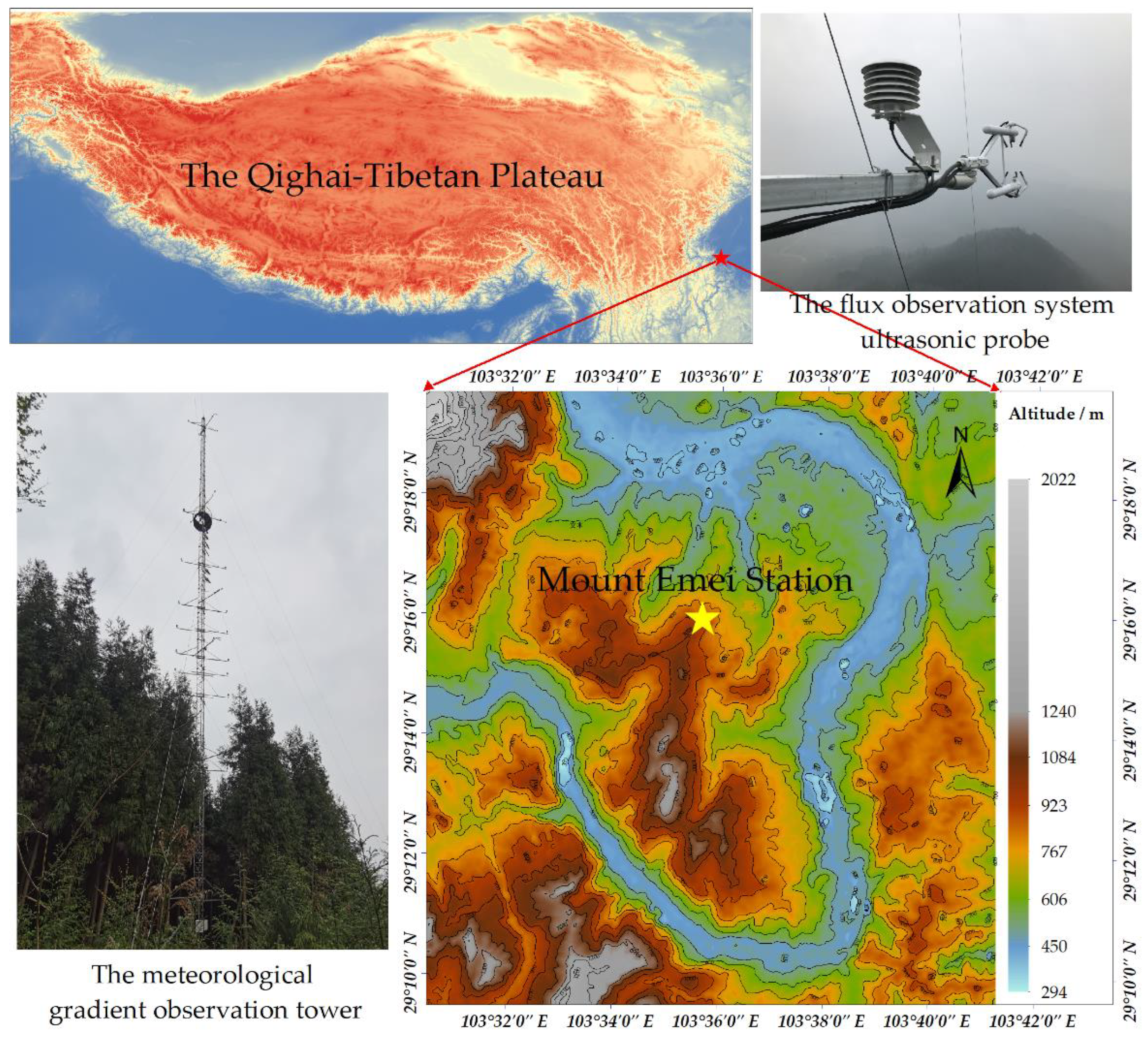
2.1. Introduction of Study Area and Data

The Emei Mountains belong to the Qionglai Mountains of the Transverse Mountain System and are divided into Mount Da’e, Mount Er’e, Mount San’e and Mount Si’e. The observations used in this paper are all from the Mount Emei Comprehensive Atmosphere and Environment Observation Experiment Station of Chengdu University of Information Engineering, which is erected at Mount Si’e (29.16° N, 103.36° E) at an altitude of 970 m. The station is hereafter referred to as the Mount Emei Station [34]. The Mount Emei station is specifically located in the village of Mount Si’e, Huluba Town, Shawan District, Leshan, Sichuan, 37.4 km southeast of the main peak of Mount Da’e, the Golden Peak, and surrounded by the Dadu River in all directions except for a relatively high elevation mountain range to its northwest, with a complex mountain forest on the lower bedding surface (Figure 1) and an average forest canopy height of 14 m. Mount Si’e belongs to the subtropical mountainous evergreen broad-leaved forest climate zone, and its climate is characterized by warm winters and hot summers with abundant precipitation.

The observation program of Mount Emei Station includes two parts: mean field and turbulence field, mainly observing the basic meteorological elements in the near-surface layer, soil temperature, soil humidity, radiation fluxes, and the momentum, heat, water vapor and $\mathrm{C}{\mathrm{O}}_2$, fluxes between the ground and air. The Mount Emei station meteorological gradient observation tower is 60 m high, and the basic meteorological elements such as wind speed, temperature and humidity are observed at 2, 10, 1, 18, 20, 22, 25, 30, 38, 56 and 58 m. Three sets of eddy covariance observation systems (Campbell CSAT3A 3D ultrasonic anemometer, EC150 infrared $\mathrm{C}{\mathrm{O}}_2$, ${\mathrm{H}}_2\mathrm{O}$ gas analyzer, and net radiation sensor CNR4) and the flux observation system ultrasonic probes were installed at 20, 38, and 56 m, respectively. The data collector is Campbell CR6Series, and the observation frequency of the eddy-motion correlation system is 10 Hz.

In this paper, observations from December 2019 to November 2020 were selected to estimate important aerodynamic and thermodynamic parameters such as zero-plane displacement, aerodynamic roughness, aerothermal roughness, momentum flux transport coefficient and sensible heat flux transport coefficient, and observations from March 2021–February 2022 were selected to analyze the variation characteristics of radiation and surface flux at this site for variance similarity analysis. (Note: the flux data of 20 and 56 m heights in 2021 are missing due to external factors, so the flux data used in this paper are all at 38 m height.) In this paper, the seasons are winter (December–February), spring (March–May), summer (June–August), and autumn (September–November). The time in this paper is Beijing time (UTC + (+0800) = Beijing time).

2.2. Method

2.2.1. Eddy Correlation Method

Eddy correlation technology is a method to calculate the covariance between the fluctuation of these meteorological elements and the vertical wind speed by using the observed meteorological elements (such as three-dimensional wind speed, temperature, water vapor, $\mathrm{C}{\mathrm{O}}_2$ concentration, etc.) and then calculate the fluxes in turbulent transport. In this paper, the TK3b software developed by the Department of Micro Meteorology of Bayreuth University in Germany is used to calculate the surface flux and evapotranspiration [35].

To ensure data reliability, after inputting the original turbulence data, data pre-processing was first performed to remove the anomalous point data with deviations greater than 5 times the standard deviation from the original data, interpolate the missing time series, and then perform flux calculation and necessary corrections. The formulas of momentum flux ($\tau$, unit: $\mathrm{W}·{\mathrm{m}}^{-2}$), sensible heat flux ($H$, unit: $\mathrm{W}·{\mathrm{m}}^{-2}$) and latent heat flux (LE, unit: $\mathrm{W}·{\mathrm{m}}^{-2}$) are as follows:

$$\tau =-\rho \overline{u^{\prime }{w}^{\prime }}$$

(1)

$$H=\rho C_p\overline{w^{\prime }{T}^{\prime }}$$

(2)

$$LE=\rho \lambda \overline{w^{\prime }{q}^{\prime }}$$

(3)

where $\rho$ is the air density (unit: $\mathrm{g}·{\mathrm{m}}^{-3}$); $\lambda$ is the latent heat of vaporization (unit: $\mathrm{J}·{\mathrm{g}}^{-1}$); $C_p$ is the specific heat at constant pressure (unit: $\mathrm{J}·{\mathrm{kg}}^{-1}·{°\mathrm{C}}^{-1}$); $u^{\prime }$, $w^{\prime }$,$T^{\prime }$ and $q^{\prime }$ are deviations of horizontal wind ($u$, unit: $\mathrm{m}·{\mathrm{s}}^{-1}$), vertical wind ($w$, unit: $\mathrm{m}·{\mathrm{s}}^{-1}$), temperature ($T$, unit: $°\mathrm{C}$), and specific humidity ($q$) from their averages over eddy covariance integration times. Finally, the calculated flux is subject to quality control and quality control evaluation. The selection of flux results adopts the quality grade evaluation system recommended in TK3 [36].

The advantage of the eddy correlation technique is that its flux is calculated directly by measuring the turbulent fluctuation values of various properties, it is based on the physical principles on which it is based, it is not limited by advection conditions, and it is more precise and reliable [37].

2.2.2. Zero Plane Displacement $d$

Zero-plane displacement $d$ (unit: $\mathrm{m}$) is an important physical quantity describing the aerodynamic characteristics of the underlying surface, which means the interaction between the air flow and the underlying surface occurs at this height. A more common method to obtain the zero-plane displacement $d$ is the Newton iteration method, which uses multi-layer wind profile observations to calculate $d$. The specific iteration formula is as follows:

$$f \left( d \right)=\frac{u_1-u_2}{u_1-u_3}-\frac{\ln \left(z_1-d\right)- \ln \left(z_2-d\right)}{\ln \left(z_1-d\right)- \ln \left(z_3-d\right)}$$

(4)

$$g \left(d\right)=d-\frac{f \left( d \right)}{f^{\prime }\left( d \right)}$$

(5)

where $z_1$,$z_2$ and $z_3$ are the heights of three observations (unit: $\mathrm{m}$); $u_1$, $u_2$ and $u_3$ are the wind speed at the corresponding height (unit: $\mathrm{m}·{\mathrm{s}}^{-1}$). First, the initial value of zero plane displacement $d$ is given, $g\left(d\right)$ is obtained, and then $d=g\left(d\right)$ is substituted into the iterative function to calculate $g\left(d\right)$. In this way, the iteration is repeated until the difference between two adjacent $g\left(d\right)$ is less than 0.001 (error), then $g\left(d\right)$ is the calculated zero plane displacement $d$ [38].

2.2.3. Aerodynamic Roughness $z_{0m}$ and Thermodynamic Roughness $z_{0h}$

Aerodynamic roughness $z_{0m}$ (unit:$\mathrm{m}$) is the height of zero plane displacement $d$ of rough elements on the wind dragging effect to reduce the wind speed to zero. It has nothing to do with the air flow but only the surface roughness condition, and the wind profile method is one of the most common methods to determine the surface roughness. It is known that under near-neutral stratification conditions, the wind speed varies with height, satisfying the logarithmic law.

$$U=\frac{u^{*}}{\kappa }\ln \left(\frac{z-d}{z_{0m}}\right)$$

(6)

where $U$ is the wind speed at $z$ (unit: $\mathrm{m}·{\mathrm{s}}^{-1}$), $u^{*}$ is friction velocity (unit:$\mathrm{m}·{\mathrm{s}}^{-1}$), both of which can be calculated by the eddy correlation method; $\kappa$ is von Karman constant (usually 0.4); $d$ is zero plane displacement. Therefore, the aerodynamic roughness $z_{0m}$ under the near neutral layer can be calculated by using $U$ and $u^{*}$.

The air thermodynamic roughness $z_{0h}$ (unit: $\mathrm{m})$ refers to the height that the temperature profile extends to the air temperature when the near-surface meets the MOST, which is more related to the surface temperature. It is related to the seasonal variation. The near-surface temperature clearance under the near neutral stratification is:

$$T-T_0=\frac{T_0}{k}\left(\ln \frac{z}{z_0}\right)$$

(7)

If $z_{0m}$ is replaced by surface thermodynamic roughness $z_{0h}$, there are:

$$z_{0h}=z{e}^{-\frac{k\left(T-T_0\right)}{T_0}}$$

(8)

where $T$ is the air temperature at the reference height (unit: $°\mathrm{C}$); $T_0$ is the surface temperature (unit: $°\mathrm{C}$); $\kappa$ is von-Karman constant (usually 0.4). Therefore, the air thermodynamic roughness $z_{0h}$ can be obtained by using $T$ and $T_0$ [39].

2.2.4. Momentum Flux Transport Coefficient $C_D$ and Sensible Heat Flux Transport Coefficient $C_H$

In this paper, the eddy correlation method is used to calculate the momentum flux transport coefficient $C_D$ and the sensible heat flux transport coefficient $C_H$. In the near-surface layer, the calculation formulas of $C_D$ and $C_H$ are as follows:

$$\overline{u^{\prime }{w}^{\prime }}=-C_D u^2$$

(9)

$$\overline{w^{\prime }{T}^{\prime }}=-C_H u \left(T_0-T\right)$$

(10)

where $\overline{u^{\prime }{w}^{\prime }}$ and $\overline{w^{\prime }{T}^{\prime }}$ are the covariance of vertical wind speed and horizontal wind speed, vertical wind speed and temperature, respectively, which are calculated by the eddy correlation method. u and T are the horizontal wind speed and temperature at the reference height, respectively. $T_0$ is the surface temperature [40]. The relative error of the observation is smaller when the wind speed is larger, and the stability of the end-flow data is also stronger, so the data with a wind speed of less than 5$\mathrm{m}·{\mathrm{s}}^{-1}$ are excluded from the calculation process.

2.2.5. Calculation Method of Surface Soil Heat Flux (TDEC)

This paper uses the heat conduction equation correction method (TDEC) designed by Yang et al. [41] to calculate soil heat flux based on soil temperature and humidity to estimate soil heat flux.

The one-dimensional heat conduction equation of soil is

$$\frac{\partial {\rho }_s{c}_{s}T}{{\partial }_t}=-\frac{\partial G}{\partial z}$$

(11)

where ${\rho }_s{C}_s$ is the soil heat flux (unit: $\mathrm{J}·{\mathrm{kg}}^{-1}·{\mathrm{K}}^{-1}$); T is the soil temperature (unit: $\mathrm{K}$); t is the time (unit: $\mathrm{s}$); G is the soil heat flux (unit:$\mathrm{W}·{\mathrm{m}}^{-2}$); $z$ is the depth of the soil (unit: $\mathrm{m}$).

By integrating the two sides of the one-dimensional heat conduction equation of soil, we can obtain

$$G\left(z\right)=G\left(Z_r\right)+\underset{Z_r}{\overset{Z}{{\displaystyle \int }}}\frac{\partial {\rho }_s{c}_{sT\left(z\right)}}{\partial t}dz$$

(12)

where $G \left(Z_r\right)$ is the soil heat flux at the soil depth of ($Z_r)$.

Given the temperature distribution profile $T\left(Z_i\right)$, Equation (13) can be expressed as

$$G=G\left(Z_r\right)+\frac{1}{\Delta t}{\displaystyle \sum }_{Z_i}^Z\left[{\rho }_s{c}_s\left(Z_i,t+\Delta t\right)T\left(Z_i,t+\Delta t\right)-{\rho }_s{c}_s\left(Z_i,t\right)T\left(Z_i,t\right)\right]$$

(13)

Taking $Z_r$ = 1 m, if the soil heat flux at 1 m is ignored, i.e., $G_{100}\approx 0$, the key to solving the equation is to obtain a more accurate temperature distribution profile T $\left(Z_i\right)$ by using limited observation data. Yang et al. [41] gave a new interpolation method, assuming that the soil heat conductivity is a fixed value of 0.5 or 1.0 $\mathrm{W}·{\mathrm{m}}^{-1}·{\mathrm{k}}^{-1}$, and then obtained the temperature profile through the soil heat diffusion equation. The observed temperature profile is used for correction to obtain a more accurate temperature profile. Therefore, the soil heat flux of each layer can be obtained by Formula (13).

2.2.6. Surface Energy Balance Equation

The surface energy balance equation is

$$H+LE=R_n-G-S-Q$$

(14)

where $H$ is the sensible heat flux; $LE$ is the latent heat flux; $R_n$ is the net surface radiation (unit: $\mathrm{W}·{\mathrm{m}}^{-2}$); $G$ is the heat flux of shallow soil (unit: $\mathrm{W}·{\mathrm{m}}^{-2}$); $S$ is the canopy heat reserve (unit: $\mathrm{W}·{\mathrm{m}}^{-2}$); $Q$ is the sum of additional energy sources and sinks (unit: $\mathrm{W}·{\mathrm{m}}^{-2}$).

Surface net radiation $R_n$ is the main energy source of energy and material exchange between the surface and atmosphere, which can be expressed as:

$$R_n=R_{SW-IN}-R_{SW-OUT}+R_{LW-IN}-R_{LW-OUT}$$

(15)

where $R_{SW-IN}$ is the total solar radiation; $R_{SW-OUT}$ is the surface reflected radiation; $R_{LW-IN}$ is atmospheric inverse radiation; $R_{LW-OUT}$ is atmospheric long wave radiation (unit: $\mathrm{W}·{\mathrm{m}}^{-2}$).

The crown thermal storage ($S$) is calculated as

$$S=S_a+S_{\lambda }+S_{leaves}-S_{trunks}$$

(16)

$$S_a=\frac{\partial }{\partial t}{{\displaystyle \int }}_0^{hc}\rho C_{\rho }\left(1+0.84\overline{q}\right)T_b{d}_Z$$

(17)

$$S_{\lambda }=\frac{\partial }{\partial t}{{\displaystyle \int }}_0^{hc}\rho \lambda q_b{T}_b{d}_Z$$

(18)

where $S_a$ is the sensible heat flux in the canopy (unit: $\mathrm{W}·{\mathrm{m}}^{-2}$), $S_{\lambda }$ is the latent heat flux in the canopy (unit:$\mathrm{W}·{\mathrm{m}}^{-2}$), $S_{leaves}$ is the leaf heat storage in the canopy (unit: $\mathrm{W}·{\mathrm{m}}^{-2}$), $S_{trunks}$ is the branch heat storage in the canopy (unit:$\mathrm{W}·{\mathrm{m}}^{-2}$), $hc$ is the canopy height (unit: $\mathrm{m}$), $q_b$ is the air humidity in the canopy, $q$ is the average air humidity in the canopy, and $T_b$ is the air temperature in the canopy (unit: $°\mathrm{C}$). Due to the lack of biological temperature observations such as leaves and branch trunks, the leaf heat storage $S_{leaves}$ and branch trunk heat storage $S_{trunks}$ were not considered in the canopy heat storage calculation [42].

Since the value of $Q$ is usually small and can be ignored in the surface energy balance equation, Equation (14) can be simplified to

$$H+LE=R_n-G-S_a-S_{\lambda }$$

(19)

where $\left(H+LE\right)$ is the turbulent flux;$\left(R_n-G-S_a-S_{\lambda }\right)$ is the effective energy.

2.2.7. Analysis Method of the Degree of Closure of the Surface Energy Balance

Currently, there are four main methods to analyze the degree of energy balance closure at the surface. They are the least squares method (ordinary least squares (OLS)), the pressure axis regression method (RMA), the energy balance ratio method (EBR), and the energy balance residual frequency distribution map method [43]. In this paper, OLS was used to discuss the degree of energy closure in the Emei Mount region. A linear regression analysis of turbulent fluxes and effective energy is performed, and the slope of the regression equation represents the degree of surface energy closure. If, ideally, the surface energy exchange reaches equilibrium, i.e., the turbulent flux and effective energy are equal, the slope of the equation should be 1 and pass through the origin.

3. Results and Analysis

3.1. Characteristics of Changes in Near-Surface Meteorological Elements

The seasonal average daily variation of temperature, humidity and wind speed at 2 and 10$\mathrm{m}$ within and 20, 38 and 58$\mathrm{m}$ above the canopy of the forest understory on Mount Emei and the variation of wind direction at each layer are given in Figure 2. It can be seen that the daily variation of temperature in the Mount Emei area has a unimodal structure. The temperature of each height layer has a minimal value at 07:00–09:00 in the morning, and the rate of warming increases and then decreases after sunrise, reaching the peak temperature of the day at 14:00–16:00, and the peak occurs later with the change in seasons, and the cooling rate in the afternoon is lower than that in the morning. The temperature difference between morning and evening is small in the Mount Emei area, and the seasonal variation is large. The average temperature is highest in summer and lowest in winter. In terms of different heights, the temperature is lowest at 58 m above the canopy, followed by 38 $\mathrm{m}$ height. The temperature values at 2 and 10 $\mathrm{m}$ height within the canopy are very close, and after sunrise, as the forest canopy absorbs solar radiation, it is slightly higher than the temperature at 20 $\mathrm{m}$ above the canopy from 12:00 to 16:00.

The Mount Emei area is surrounded by rivers on three sides, and the overall relative humidity is high, basically above 60% throughout the year. As can be seen from Figure 2b, the relative humidity of all layers near the ground at the site has an asymmetric “V” shape. The relative humidity of each height layer is larger from 00:00 to 08:00 and changes more slowly, during which the maximum relative humidity of the day occurs, and then the relative humidity decreases rapidly after sunrise and decreases to the minimum relative humidity of the day from 17:00 to 19:00 in the evening. There are noteworthy seasonal variations in relative humidity, and the relative humidity in autumn and winter is much higher than that in spring and summer, especially in autumn, when the average relative humidity in all layers is above 80%. In addition, the relative humidity within the canopy was greater than that above the canopy, partly because the canopy cut the wind speed blowing across the ground and reduced air flow, which played a role in moisture retention. Overall the lower layers were relatively moist and the upper layers relatively dry.

From Figure 2c, it can be seen that the wind speed near the ground shows the characteristics of high wind speed at the upper level and low wind speed at the lower level. The daily variation of wind speed at the upper levels of the site is more significant than that at the lower levels, with an irregular flat “W” pattern. The wind speed at 20, 38, and 58 $\mathrm{m}$ height on the canopy is much higher than that at 2 and 10 $\mathrm{m}$ height in the canopy, and the wind speed on the canopy has a similar trend, increasing and then decreasing from 00:00 to 12:00, with small fluctuations during the period. The maximum wind speed of the day was observed. In the afternoon, there was a decreasing–increasing process, and the wind speed decreased to the minimum value of that day, but the wind speed at 38 and 58 $\mathrm{m}$ was still much larger than that at 20$\mathrm{m}$. The wind speed at 2 and 10 m in the canopy was much higher than that at 20 m. The daily variation of wind speed at 2 and 10 $\mathrm{m}$ height in the canopy is not significant, which is due to the canopy shading, but it can still be seen that there is a minimum value of wind speed between 18:00 and 19:00, and the average wind speed at night is greater than that during the day. The variation of wind speed at each layer was significantly greater in spring and summer than in autumn and winter, especially in summer.

Figure 2d shows the rose diagram of wind frequency per 30 min at 2 and 10$\mathrm{m}$ in the canopy and 20, 38 and 58$\mathrm{m}$ in the upper canopy in the Mount Emei area. WSW, W, WNW wind direction together called west wind, and NNW, N, NNE and NE wind direction together called north wind. The figure shows that the west wind is dominant at 2, 10 and 20$\mathrm{m}$ height, with 43.6%, 43.6% and 32.94%, respectively, and the north wind is the second dominant wind at 20$\mathrm{m}$ height, with 24.85%. At 38$\mathrm{m}$ height, the north wind is the dominant wind, accounting for 34.1%, while the west wind is the second dominant wind direction, accounting for 27.1%, which shows that the west wind is absolutely dominant in high wind greater than or equal to 6 $\mathrm{m}·{\mathrm{s}}^{-1}$.

3.2. Aerodynamic and Thermodynamic Parameters

3.2.1. Zero Plane Displacement $d$, Aerodynamic Roughness $z_{0m}$ and Thermodynamic Roughness $z_{0h}$

It can be seen from the scatter diagram of the annual distribution and the monthly variation of its average value of zero plane displacement $d$, aerodynamic roughness $z_{0m}$ and aerothermodynamic roughness $z_{0h}$ (Figure 3) that the dispersion of $d$ is generally high, 80% of $d$ is 8~19 $\mathrm{m}$, the monthly average value fluctuates between 9.5 and 11.5 $\mathrm{m}$, the maximum value is 11.4 $\mathrm{m}$ in February and the minimum value is 9.52 $\mathrm{m}$ in October, and the final annual average value of zero plane displacement $d$ is 10.45 $\mathrm{m}$. The dispersion of $z_{0m}$ is also high, but more than 90% of the data are concentrated in 0~2 $\mathrm{m}$. The annual aerodynamic roughness fluctuates greatly with seasons, and its value is large in autumn, with a maximum value of 2.33 $\mathrm{m}$ in September. Its value is small in winter and has a minimum value of 0.90 m in December. The annual average dynamic roughness is 1.61 $\mathrm{m}$. The distribution of $z_{0h}$ is relatively concentrated on the whole, ranging from 1 to 2 m. The fluctuation of air thermodynamic roughness with seasons is small, and the annual average value is 1.67$\mathrm{m}$.

3.2.2. The Momentum Flux Transport Coefficient $C_D$ and the Sensible Heat Flux Transport Coefficient $C_H$

Through calculation, the distribution of the momentum flux transport coefficient $C_D$ and sensible heat flux transport coefficient $C_H$ with time, monthly average change and distribution with wind speed are obtained (Figure 4). The annual momentum flux transport coefficient $C_D$ distribution with time is relatively scattered, but more than 95% of the values are 0~0.05. From the perspective of monthly variation, the momentum flux transport coefficient $C_D$ fluctuates less in spring and summer and more in autumn and winter, with a maximum value of 0.0228 in October. The distribution of sensible heat flux transport coefficient $C_H$ with time is also relatively scattered, but more than 90% of the value is 0~0.01. The sensible heat flux transport coefficient $C_H$ is smaller in summer, larger in spring and autumn in October, and has a maximum value of 0.00467 in March. Momentum flux transport coefficient $C_D$ and sensible heat flux transport coefficient $C_H$ have similar variation characteristics with wind speed. When the wind speed is small, they both increase with the decrease in wind speed. When the wind speed is less than 6 $\mathrm{m}·{\mathrm{s}}^{-1}$, the $C_H$ value becomes more scattered. When the wind speed is large, they both decrease with the increase in wind speed, and $C_D$ gradually tends to a constant value with the increase in wind speed. The annual average values of momentum flux transport coefficient $C_D$ and sensible heat flux transport coefficient $C_H$ are $1.58\times {10}^{-2}$ and $3.79\times {10}^{-3}$, respectively.

Table 1. Comparison of overall transport coefficient under different underlying surfaces.

Observation Site	Wind Direction	Canopy Height/m	$\mathit{d}/\mathbf{m}$	${\mathit{z}}_{0\mathit{m}}/\mathbf{m}$	${\mathit{C}}_{\mathit{D}} \mathbf{(}\mathbf{\times }{\mathbf{10}}^{\mathbf{-}\mathbf{3}}\mathbf{)}$	${\mathit{C}}_{\mathit{H}} \mathbf{(}\mathbf{\times }{\mathbf{10}}^{\mathbf{-}\mathbf{3}}\mathbf{)}$	Source
Changbai Mountain	/	26	19.5	1.60	6.66	6.4	[44]
Gaize	/	0.05	/	/	2.31	2.15	[27]
Phoenix Mountain	315°~45°	18	30.29	1.80	50	5.5	[45]
Phoenix Mountain	45°~135°	18	8.24	0.67	5.5	3.0	[45]
Phoenix Mountain	135°~225°	18	16.46	1.35	22	4.0	[45]
Phoenix Mountain	225°~315°	18	/	/	/	/	[45]
Emei Mount	/	14	10.45	1.65	15.8	3.79	this paper

shows the experimental results of momentum flux transport coefficient $C_D$ and sensible heat flux transport coefficient $C_H$ on different underlying surfaces. Through comparison, it is found that there is a large difference between momentum flux transport coefficient $C_D$ and sensible heat flux transport coefficient $C_H$ on different underlying surfaces, and it varies with the wind direction. The calculated results of momentum flux transport coefficient $C_D$ and sensible heat flux transport coefficient $C_H$ in Changbai Mountain are greater than those in Mount Emei, which is determined by the different roughness of the underlying surface caused by different forest canopy heights.

3.3. The Similarity Relationship of Dimensionless Wind Speed Fluctuation Variance

According to MoninObukhov similarity theory, the fluctuation variance (${\sigma }_a/u^{*}, a=u, v, w$) of near formation wind is a function of stability parameter $z/L$ after dimensionless friction velocity ($u^{*}$), that is:

$${\sigma }_a/u^{*}={\mathsf{\Phi }}_a(z/L) a=u, v, w$$

(20)

where ${\mathsf{\Phi }}_{\mathrm{a}}$ is the universal function of wind fluctuation variance. $L$ is the Obukhov length, which characterizes the vertical scale of turbulent mixing.

Figure 5 shows the variation of dimensionless wind fluctuation variance with stability parameter $z/L$. The solid line in the figure is the curve of the universal function obtained by fitting, and the corresponding function form is as follows:

$${\sigma }_u/u^{*}=2.591{\left(1-3.993Z/L\right)}^{0.2396} z/L<0$$

(21)

$${\sigma }_v/u^{*}=1.684{\left(1-155.1Z/L\right)}^{0.1639} z/L<0$$

(22)

$${\sigma }_w/u^{*}=1.314{\left(1-3.199Z/L\right)}^{0.3338} z/L<0$$

(23)

It can be seen that under the unstable stratification, the dimensionless vertical wind fluctuation variance in the Mount Emei area can better conform to the 1/3 power law of Monin–Obukhov similarity theory, while the dimensionless horizontal wind fluctuation variance does not conform to the 1/3 power law of Monin–Obukhov similarity theory. This is caused by the topographic relief and the difference in the physical characteristics of the underlying surface. The underlying surface is mountainous forest, and the topographic relief is much larger than that of the plain, which affects the horizontal turbulence movement, while the topographic relief and the difference in the physical characteristics of the underlying surface have less influence on the vertical turbulence. Under stable conditions, the distribution of the dimensionless wind fluctuation variance with the stability parameters is relatively discrete, which does not conform to the 1/3 power law of Monin–Obukhov similarity theory. Li et al. [46] and Liuet al. [47] also found that the similarity relationship under the unstable stratification is good, while the relationship under the stable stratification disappears. The reason may be that the stability increases to a certain extent, and the atmospheric fluctuation, intermittent turbulence, etc., cause it to deviate from the similar law. In the case of near neutral, there is almost no thermal effect in the near-surface layer, and the turbulence is mainly generated by mechanical turbulence. The above dimensionless velocity variance is approximately equal to the constant in the case of near neutral, that is:

$${\sigma }_u/u^{*}=A,{\sigma }_v/u^{*}=B,{\sigma }_w/u^{*}=C$$

(24)

where $A$, $B$ and $C$ are constants. Because the dimensionless horizontal wind fluctuation variance under unstable stratification in this study does not conform to the 1/3 power law of Monin–Obukhov similarity theory, the values of $A$ and $B$ are not discussed. According to the above fitted similarity function, the $C$ value of the Mount Emei area is 1.314. Compared with the research results of different underlying surfaces and different times in other areas (

Table 2. The dimensionless wind speed fluctuation variance under near neutral stratification of different underlying surfaces.

Site	Observation Time	Canopy Height	Observation Height	${\mathit{\sigma }}_{\mathit{u}}/{\mathit{u}}^{*}=\mathit{A}$	${\mathit{\sigma }}_{\mathit{v}}/{\mathit{u}}^{*}=\mathit{B}$	${\mathit{\sigma }}_{\mathit{w}}/{\mathit{u}}^{*}=\mathit{C}$	Source
Mount Emei	December 2019–November 2020	14	38	/	/	1.314	this paper
Xiaolangdi plantation observation area	2015. Spring	10.1	30	3.31	3.17	1.84	[48]
	2016. Summer	10.1	30	2.04	2.62	1.57	[48]
Changbai Mountain	September 2003	26	42	2.47	2.47	1.47	[49]
Gaize	June–July 1998	0.05	2.57	3.21	2.69	1.46	[27]
Wudaoliang	June–July 1994	0.05	2.9	2.98	2.91	1.35	[50]
Plain area	/	/	/	2.4	1.9	1.25	[51]
Litang	January 2006	0.05	4	3.7	3.29	0.92	[19]
Litang	July 2006	0.05	4	4.44	4.28	0.96	[19]
Jinta Oasis, Gansu	June–August 2008	1–2	10	2.4	2.5	1.3	[52]
Jinta Gobi, Gansu	June–August 2008	1–2	1.84	2.8	2.7	1.1	[52]
Anduo	July 1998	0.05	2.9	4.01	3.85	1.43	[30]

), the C value in the Mount Emei area is close to that in most areas.

3.4. The Variation Characteristics of Surface Energy

3.4.1. The Variation Characteristics of Each Component of Surface Balance

Figure 6 shows the seasonal average variation of each component of the surface balance of Mount Emei station in each season. It can be seen from the figure that the diurnal and seasonal changes in each component of the surface balance are significant. The diurnal variation of net radiation is unimodal, and its value increases rapidly after sunrise. It is positive most of the time, reaches the maximum value from 12:00 to 14:00, and becomes negative about before sunset; The minimum value is reached within two hours after sunset (about 19:00). The seasonal variation difference in net radiation is mainly in the daytime. The net radiation is the strongest in spring and summer. The daily maximum exceeds 500 $\mathrm{W}·{\mathrm{m}}^{-2}$, the highest reaches 541.77$\mathrm{W}·{\mathrm{m}}^{-2}$, and the weakest in winter. The average daily variation extreme value is 260.58 $\mathrm{W}·{\mathrm{m}}^{-2}$. Soil heat flux refers to the energy transmitted between the surface and deep soil, which is an important part of the surface heat balance. The diurnal variation trend of soil heat flux is the same as that of net radiation, but the value is much smaller than that of net radiation. The dominant position of sensible heat flux and latent heat flux in the daytime varies significantly with seasons, and the sensible heat flux in spring is slightly greater than the latent heat flux. In summer, the subsurface bedding has a large vegetation cover, the transpiration of the vegetation takes away a large amount of water vapor, and the latent heat flux is greatly enhanced and dominant. The dominant position of latent heat flux decreased gradually in autumn, and there was little difference between sensible heat flux and latent heat flux. In winter, the transpiration of vegetation decreases, the sensible heat transport during the day is greater than the latent heat transport, and the sensible heat transport is dominant. In addition, the sensible heat and latent heat in this area have significant diurnal variation rules, both of which show a single peak structure. After sunrise, with the heating of the surface by solar radiation, the sensible heat flux in Mount Emei began to increase at about 6:30, and the sensible heat value was positive, indicating that the surface transported heat to the atmosphere by sensible heat, peaked at about 13:30, and then began to decrease gradually. After sunset, because the surface radiation began to cool at about 18:30, the sensible heat value became negative, indicating that the atmosphere transported heat to the surface, and the daily variation range was much greater in the daytime than at night. The latent heat flux is positive throughout the day, indicating that energy is transferred from the ground to the atmosphere.

3.4.2. Surface Radiation Budget Characteristics

Figure 7 shows the seasonal average daily variation of each component of the surface radiation balance. The surface radiation budget in the Mount Emei area is mainly $R_{SW-IN}$ and $R_{SW-OUT}$, and its radiation components have very significant characteristics of daily variation and seasonal variation. $R_{SW-IN}$ is the amount of solar radiation reaching the ground after atmospheric absorption and scattering. $R_{SW-IN}$ is affected by solar altitude angle and atmospheric transparency, The larger the solar altitude angle, the larger the $R_{SW-IN}$. The higher the atmospheric transparency, the higher the ${\mathrm{R}}_{SW-IN}$. The daytime solar altitude angle is large, and the $R_{SW-IN}$ value is large. The solar altitude angle at night is 0, and the $R_{SW-IN}$ value is 0. $R_{SW-IN}$ and $R_{LW-OUT}$ are much higher in spring and summer than in autumn and winter. The average daily variation extremes of $R_{SW-IN}$ in both spring and summer exceed 500 $\mathrm{W}·{\mathrm{m}}^{-2}$, up to 613.61 $\mathrm{W}·{\mathrm{m}}^{-2}$. The total solar radiation in winter is the smallest, and the average daily variation maximum is only 132.6 $\mathrm{W}·{\mathrm{m}}^{-2}$. Moreover, due to the change in solar altitude angle in spring and summer, the time when $R_{SW-IN}$ begins to increase is earlier than that in autumn and winter, and the time when $R_{SW-IN}$ begins to decrease in the evening lags behind that in autumn and winter.$R_{LW-OUT}$ is the reflection of the surface to $R_{SW-IN}$. The daily variation law is consistent with ${\mathrm{R}}_{SW-IN}$, but the magnitude is very different from $R_{SW-IN}$. $R_{LW-IN}$ is the long wave radiation incident on the earth’s surface through the whole atmosphere. Its change is mainly affected by temperature, cloud, carbon dioxide, water vapor and aerosol. Secondly, altitude and geographical latitude also have a certain impact on the long wave downward radiation [53]. The higher the altitude, the lower the air pressure and the smaller the water vapor content, the lower the $R_{LW-IN}$ value. During the day,$R_{LW-IN}$ is always kept within a certain range, with relatively gentle daily variation, amplitude far less than other radiation components, and significant seasonal variation. In winter, due to low temperature and water vapor content, $R_{LW-IN}$ is far less than that in other seasons. The $R_{LW-IN}$ emitted and reflected by the surface is $R_{LW-OUT}$, which is mainly affected by the surface temperature. The daily variation characteristics are consistent with the temperature variation characteristics.$R_{LW-OUT}$ is the smallest in winter and the largest in summer.

The daily variation of each component presents a single peak structure. Before sunrise, $R_{SW-IN}$ and $R_{SW-OUT}$ were zero. After 8:00, $R_{SW-IN}$ and $R_{SW-OUT}$ gradually increased, peaked between 14:00 and 15:00, began to decrease gradually, and decreased to zero around 18:30. After sunrise, due to the rise of temperature, $R_{LW-IN}$ and $R_{LW-OUT}$ also began to rise, but the rise range was small, with a peak around 14:00. Then it began to decrease slowly. At night, due to the cooling of surface and atmospheric radiation, the long wave radiation value is small, and it is the valley value of long wave radiation before sunrise.

3.4.3. Variation Characteristics of Surface Albedo

Table 3. Surface reflectance of stations in northern Tibet Plateau and Mount Emei station in each season.

Site (Underpad Surface)	Longitude and Latitude	Altitude	Spring	Summer	Autumn	Winter	Source
D105 (alpine Grassland)	32.69° N, 91.94° E	5020 m	0.28	0.22	0.23	0.32	[56]
Anduo (alpine Grassland)	32.24° N, 91.64° E	4700 m	0.27	0.22	0.23	0.33	[56]
Naqu (alpine Grassland)	31.37° N, 91.90° E	4534 m	0.24	0.18	0.18	0.35	[56]
Pailong (gravel and grass)	30.04° N, 95.61° E	2058 m	0.14	0.13	0.14	0.14	[33]
Danka (grass)	29.89° N, 95.68° E	2701 m	0.14	0.13	0.14	0.17	[33]
Mount Emei (grass)	29.52° N, 103.34° E	3070 m	0.18	0.16	0.18	0.31	[33]
Mount Emei (forest)	29.52° N, 103.34° E	970 m	0.07	0.06	0.06	0.04	This paper

shows the average value of the average surface albedo in the daytime of each season in Mount Emei. It can be seen that the surface albedo in the daytime of each season in this area has little difference, ranging from 0.05 to 0.08, which is closely related to the fact that this area is an evergreen forest in all seasons. However, the surface albedo in winter is slightly lower than that in other seasons, which is 0.05 and is related to the phenological changes in forest canopy leaves [54]. Due to the difference in climate and underlying surface properties in the observation area, the influence of latitude and altitude on surface albedo is also different. Table 3 also lists the surface albedo of some stations on the Qinghai Tibet-Plateau and under the grass bedding surface at different elevations of Mount Emei. Under the same underlying surface, the difference in surface albedo between stations at different altitudes is within 0.05, while the surface albedo of stations with higher altitude underlying surface of alpine meadow is significantly higher than that of stations with underlying grassland surface, and much higher than that of stations with underlying forest surface. The difference between the surface albedo of alpine meadow and grass underlay sites and that of forest underlay sites in this paper is more than 0.1. When the altitude is similar, the higher the northern latitude, the greater the ground albedo, which is consistent with the conclusion of Zhong et al. [55]. In addition, except for the Mount Emei Station (forest), the surface albedo of other stations on the plateau in winter is higher than that in other seasons, which is due to the snowy weather at other stations in winter. It can be seen that the influence of the underlying surface on the surface albedo is far greater than other factors such as altitude, longitude and latitude.

3.4.4. Characteristics of Changes in the Degree of Energy Balance Closure

The problem of near-surface energy closure (the sum of sensible and latent heat fluxes is generally always smaller than the effective energy), especially the energy closure in the forest subsurface, has been one of the difficulties in the study of land–air interaction processes for many years. An analysis of the degree of energy balance closure in the Mount Emei region shows that the non-closure phenomenon is very significant in the region. Figure 8 depicts the changes in near-surface energy closure at Mount Emei station before and after considering canopy thermal storage. Before considering canopy thermal storage, the energy closure at Mount Emei station is 46%, and the correlation coefficient $R^2$ is 0.68. After considering canopy storage, the energy closure increases to 48%. It can be seen that the influence of the sensible heat flux $S_a$ in the canopy and the latent heat flux $S_{\lambda }$ in the canopy on the surface energy balance is small, and although the influence of Sa and S_λ on the energy closure rate is considered, there is still an energy imbalance of about 52%. This indicates that the energy balance problem in the forest understory is complex and there are still some other energy transfer mechanisms to be considered, such as the local vertical circulation over the forest or the storage of energy by the leaves and canopy of the forest canopy, etc.

Table 4. Energy closure rate between some stations in Qinghai-Tibet Plateau and Mount Emei station.

Observation Site	Longitude and Latitude	Altitude/m	Underpad Surface	Closure Rate/%	Source
Nyainrong Station	32.17° N, 92.30 E	4607	alpine grassland	74.0	[57]
Nagqu Station	32.37 N, 91.90 E	4509	alpine grassland	66.4	[58]
Dangxiong Grassland Station	30.51 N, 91.05 E	4333	alpine meadows	53.0	[59]
Everest Station	28.36 N, 86.95 E	4276	river beach sand and gravel grass	40.0	[58]
Pai Lung Station	30.04 N, 95.61 E	2058	gravel and grass	57.2	[33]
Emei Mountain (grass)	29.52 N, 103.34 E	3070	grass	64.5	[33]
Emei Mountain (forest)	29.16 N, 103.36 E	970	forest	48	This paper

shows the energy closure rates of some stations on the Qinghai-Tibet Plateau and Mount Emei station, and it can be seen that all stations have different degrees of energy non-closure. The energy closure rates of different types of substrates vary widely, with the grass substrates having high closure rates above 60% and the forest substrates and riverbank gravel substrates having the lowest closure rates. Lv et al. [33] derived a daytime closure rate of 67.22% for the Mount Emei area (grassland sub-bedding surface) in winter, which is different from the results obtained in this paper (forest sub-bedding surface and is due to the different sub-bedding surfaces.

Combined with the specific situation of the surface of Mount Emei station, preliminary analysis of the possible reasons for its energy non-closure are mainly as follows. First, the study area of this paper is a forest understory with dense vegetation in all seasons, and the plant canopy heat storage accounts for a considerable proportion of the heat storage. In this paper, due to the lack of biological temperature observation data such as leaves and branch trunks, the leaf heat storage and branch trunk heat storage in the canopy are not considered; second, the soil heat flux calculated by the TDEC method in this paper, which uses multi-layer soil temperature and humidity for calculation, has better estimation results compared with other methods. However, it also assumes the soil thermal conductivity to estimate the soil heat flux, which also has errors with the actual soil heat flux, plus seasonal changes and vegetation cover, etc. The soil thermal conductivity is more complex, and the estimated soil heat flux has more significant errors, which has a greater impact on the degree of energy balance closure. Third, ignoring the advection term will affect the closure of the energy balance. The location of the flux station requires that the underlying surface is a large and flat homogeneous source area, but this condition is difficult to meet in the field, leading to the widespread advection phenomenon. In the vortex-related technology flux observation, it is generally believed that the vertical advection can be ignored by rotating the coordinates so that the vertical wind speed is zero. However, in fact, when the air flows through the observation station, there is an upward or downward air flow, and vertical advection will occur. In addition, horizontal advection of air with uneven temperature levels under the action of a wind field will also cause horizontal heat transfer near the ground, which will lead to changes in the heat budget in a unit air block. Lu et al. [60] found that the contribution of near-surface horizontal advection to the near-surface energy closure of Zoige alpine wetland in summer is 5.8%, which shows that the horizontal advection has a great impact on the near-surface energy closure. Since no more than two flux observation towers are observed in parallel in this observation, the loss amount cannot be obtained.

4. Conclusions

Based on the ABL gradient tower data, the radiation observation data of an automatic weather station and the surface flux data of Mount Emei station on the eastern edge of Qinghai Tibet Plateau from December 2019 to November 2020 and from March 2021 to February 2022, the components of surface equilibrium are estimated by eddy correlation method and TDEC method, the characteristics of surface energy exchange in the Mount Emei area are analyzed, and the important aerodynamic and thermodynamic parameters such as zero plane displacement, aerodynamic roughness, aerothermal roughness, momentum flux transport coefficient and sensible heat flux transport coefficient are estimated. The main conclusions are as follows:

(1)

The annual average value of zero-plane displacement $\mathrm{d}$ calculated is 10.45 $\mathrm{m}$. Aerodynamic roughness basically does not change with seasons, and aerodynamic thermal roughness fluctuates slightly with seasons. The annual average values of aerodynamic roughness $z_{0m}$ and aerothermal roughness $z_{0h}$ obtained by calculation are 1.65 and 9.95 $\mathrm{m}$, respectively. The annual average values of momentum flux transport coefficient $C_D$ and sensible heat flux transport coefficient $C_H$ are $1.58\times {10}^{-2}$ and $3.79\times {10}^{-3}$, respectively.

(2)

Under unstable stratification, the dimensionless vertical wind fluctuation variance in the Mount Emei area can better conform to the 1/3rd power law of Monin–Obukhov similar theory, while the dimensionless horizontal wind fluctuation variance does not conform to the 1/3rd power law of Monin–Obukhov similar theory. This is caused by the topographic relief and the difference in the physical characteristics of the underlying surface. Under the stable stratification condition, the dimensionless wind fluctuation variance does not conform to the 1/3 order law of Monin–Obukhov similar theory. In the near-neutral case, the dimensionless velocity variance in the vertical direction in this area is 1.314.

(3)

The sensible heat flux in spring is slightly greater than the latent heat flux, the latent heat flux in summer is dominant, the dominant position of latent heat flux in autumn is gradually reduced, the difference between sensible heat flux and latent heat flux is small, and the sensible heat flux in winter is dominant.

(4)

The average surface albedo of the Mount Emei area in each season in the daytime has little difference, ranging from 0.05 to 0.08. The surface albedo in winter is slightly smaller than that in other seasons, which is 0.05. The station is a forest underlay, so its albedo is less than most stations on the plateau.

(5)

The non-closure phenomenon is significant in the Mount Emei area. Before considering the canopy thermal storage, the energy closure rate of the Mount Emei station was 46%, and after considering the canopy thermal storage, the energy closure rate increased to 48%. The possible reason for the energy non-closure in this area is that the influence of horizontal advection and vertical advection on the energy closure is not considered. Second, consider the effects of the leaf heat storage, branch heat storage in the canopy on the energy closure, and the more significant errors in the estimated soil heat fluxes.

This study only makes a preliminary analysis of the characteristics of surface flux in the Mount Emei area. Further long-term observation and research are needed to deeply understand the earth–atmosphere interaction in this area.

References

1. Stull, R.B. An Introduction to Boundary Layer Meteorology; Kluwer Academic Publishers: Boston, MA, USA, 1988; pp. 3–666. [Google Scholar]
2. Ding, A.J. Study on Variation Characteristics and Transport of Air Pollutants at Low Level in East Asia. Ph.D. Thesis, Nanjing University, Nanjing, China, 2004. [Google Scholar]
3. Wu, G.X.; Liu, X.; Zhang, Q.; Qian, Y.F.; Mao, J.Y.; Liu, Y.M.; Li, W.P. Progresses in the Study of the Climate Impacts of the Elevated Heating over the Tibetan Plateau. Clim. Environ. Res. 2002, 7, 184–201. [Google Scholar]
4. Duan, A.M.; Wu, G.X. Weakening trend in the atmospheric heat source over the Tibetan Plateau during recent decades. Part I: Observations. J. Clim. 2010, 21, 3149–3164. [Google Scholar] [CrossRef] [Green Version]
5. Yang, K.; Wu, H.; Qin, J.; Lin, C.G.; Tang, W.J.; Chen, Y.Y. Recent climate changes over the Tibetan Plateau and their impacts on energy and water cycle: A review. Glob. Planet Chang. 2014, 112, 79–91. [Google Scholar] [CrossRef]
6. Wilson, K.; Goldstein, A.; Falge, E.; Aubinet, M.; Baldocchi, D.; Berbigier, P.; Bernhofer, C.; Ceulemans, R.; Dolman, H.; Field, C.; et al. Energy balance closure at FLUXNET sites. J. Agric. Meteorol. 2002, 113, 223–243. [Google Scholar] [CrossRef] [Green Version]
7. Foken, T.; Wimmer, F.; Mauder, M. The Energy Balance Closure Problem: An Overview. Ecol. Appl. 2008, 18, 1351–1367. [Google Scholar] [CrossRef]
8. Oncley, S.; Foken, T.; Vogt, R.; Kohsiek, W.; DeBruin, H.A.; Bernhofer, C.; Christen, A.; Van Gorsel, E.; Grantz, D.; Feigenwinteret, C.; et al. The energy balance experimentEBEX-2020. Part I: Overview and energy balance. Bound.-Layer Meteor. 2007, 123, 1–28. [Google Scholar] [CrossRef]
9. Jacobs, A.; Heusinkveld, B.; Holtslag, A. Towards closing the surface energy budget of a mid-latitude grassland. Int. J. Climatol. 2010, 9, 30. [Google Scholar] [CrossRef] [Green Version]
10. Xu, X.D.; Chen, L.S. Advances of the Study on Tibetan Plateau Experiment of Atmospheric Sciences. J. Appl. Meteor. Sci. 2006, 6, 756–772. [Google Scholar]
11. Li, D.L.; Zhang, J.J.; Wu, H.B. A diagnostic study on surface sensible heat flux anomaly in summer over the Qinghai-Xizang Plateau. Plateau Meteor. 1997, 16, 367–375. [Google Scholar]
12. Li, G.P.; Duan, T.Y.; Wu, G.F. The Intersity of Surface Heat Source and Surface Heat Balance on the Western Qinghai-Xizang Plateau. Sci. Geogr. Sin. 2003, 23, 13–18. [Google Scholar]
13. Ma, Y.M.; Yao, T.D.; Wang, J.M. Experimental Study of Energy and Water Cycle in Tibetan Plateau--The Progress Introduction on the Study of GAME/Tibet and CAMP/Tibet. Plateau Meteor. 2006, 25, 344–351. [Google Scholar]
14. Li, M.S.; Ma, Y.M.; Hu, Z.Y.; Ma, W.Q.; Wang, J.M.; Ogino, S. Study on Characteristics of ABL over Naqu Region of Northern Tibetan Plateau. Plateau Meteor. 2004, 23, 728–773. [Google Scholar]
15. Li, M.S.; Yang, Y.X.; Ma, Y.M.; Sun, F.L.; Chen, X.L.; Wang, B.B.; Zhu, Z.K. Analyses on Turbulence Data Control and Distribution of Surface Energy Flux in Namco Area of Tibetan Plateau. Plateau Meteor. 2012, 31, 875–884. [Google Scholar]
16. Chen, X.L.; Ma, Y.M.; Li, M.S.; Ma, W.Q.; Wang, H. Analyses on Near Surface Layer Atmospheric Characteristics and Soil Features in Northern Tibetan Plateau. Plateau Meteor. 2008, 27, 941–948. [Google Scholar]
17. Li, M.S.; Babel, W.; Tanaka, K.; Foken, T. Note on the application of planar-fit rotation for non-omnidirectional sonic anemometers. Atmos. Meas. Tech. 2012, 5, 7323–7340. [Google Scholar] [CrossRef] [Green Version]
18. Li, M.S.; Ma, Y.M.; Sun, F.L.; Zhao, Y.Z.; Wang, Y.J.; Lv, Y.Q. Characteristics of Micrometeorology and Exchange of Surface Energy in the Namco Region. Plateau Meteor. 2008, 27, 727–732. [Google Scholar]
19. Li, Y.; Li, Y.Q.; Zhao, X.B. Analyses of turbulent fluxes and micrometeorological characteristics in the surface layer at Litang of the eastern Tibetan Plateau. Acta Meteor. Sin. 2009, 67, 417–425. [Google Scholar]
20. Zhao, X.B.; Liu, C.W.; Tong, B.; Li, Y.B.; Wang, L.L.; Ma, Y.M.; Gao, Z.Q. Study on Surface Process Parameters and Soil Thermal Parameters at Shiquanhe in the Western Qinghai-Xizang Plateau. Plateau Meteor. 2021, 40, 711–723. [Google Scholar]
21. Fu, W.; Li, M.S.; Yin, S.C.; Lv, Z.; Wang, L.Z.; Shu, L. Study on the ABL Structure of the QinghaiXizang Plateau under the South Branch of the Westerly Wind and the Plateau Monsoon Circulation Field. Plateau Meteor. 2022, 41, 190–203. [Google Scholar]
22. Gromke, C.; Manes, C.; Walter, B.; Lehning, M.; Guala, M. Aerodynamic Roughness Length of Fresh Snow. Bound.-Layer Meteorol. 2011, 141, 21–34. [Google Scholar] [CrossRef] [Green Version]
23. Kubota, A.; Sugita, M. Radiometrically determined skin temperature and scalar roughness to estimate surface heat flux. Part I: Parameterization of radiometric scalar roughness. Bound.-Layer Meteorol. 1994, 69, 397–416. [Google Scholar] [CrossRef]
24. Graf, A.; Boer, A.; Moene, A.; Vereecken, H. Intercomparison of Methods for the Simultaneous Estimation of Zero-Plane Displacement and Aerodynamic Roughness Length from Single-Level Eddy-Covariance Data. Bound.-Layer Meteorol. 2014, 151, 373–387. [Google Scholar] [CrossRef]
25. Babić, N.; Večenaj, Ž.; De Wekker, S.F.J. Flux–Variance Similarity in Complex Terrain and Its Sensitivity to Different Methods of Treating Non-stationarity. Bound.-Layer Meteorol. 2016, 159, 123–145. [Google Scholar] [CrossRef]
26. Monin, A.S.; Obukhov, A.M. Dimensionless characteristics of turbulence in the atmospheric surface layer. Dokl. Akad. Nauk SSSR 1953, 93, 223–226. [Google Scholar]
27. Liu, H.Z.; Hong, Z.X. Turbulent Characteristics in the Surface Layer over Gerze Area in the Tibetan Plateau. Chinese J. Atmos. Sci. 2000, 24, 289–300. [Google Scholar]
28. Chen, Y.G.; Zhang, Y.; Wang, S.Y. Seasonal variation of turbulence characteristics over alpine meadow ecosystem. Plateau Meteor. 2014, 33, 585–595. [Google Scholar]
29. Liwei, Y.A.N.G.; Xiaoqing, G.A.O.; Xiaoying, H.U.I.; Na, G.A.O.; Ya, Z.H.O.U.; Xuhong, H.O.U. Study on turbulence characteristics in the atmospheric surface layer over Nyainrong grassland in central Qinghai-Tibetan Plateau. Plateau Meteor. 2017, 36, 875–885. [Google Scholar]
30. Ma, Y.; Ma, W.; Hu, Z.; Li, M.; Wang, J.; Ishikawa, H.; Tsukamoto, O. Similarity analysis of atmospheric turbulent intensity over grassland surface of Qinghai-Xizang Plateau. Plateau Meteor. 2002, 21, 514–517. [Google Scholar]
31. Franceschi, M.D.; Zardi, D.; Tagliazucca, M.; Tampieri, F. Analysis of second-order moments in surface layer turbulence in an Alpine valley. Q. J. R. Meteorol. Soc. 2010, 135, 1750–1765. [Google Scholar] [CrossRef]
32. Li, Y.; Li, Y.Q.; Zhao, X.B. The Comparison and Analysis of ABL observational data between the East of Tibetan Plateau and Chengdu Plain (I). Plateau Mt. Meteor Res. 2008, 28, 30–35. [Google Scholar]
33. Lv, Z.; Li, M.S.; Liu, X.R.; Yin, S.C.; Song, X.Y.; Fu, W.; Wang, L.Z.; Shu, L. Characteristics of Surface Energy Exchange in Emei Mountain Area on the Eastern Qinghai-Tibetan Plateau in Winter. Plateau Meteor. 2020, 39, 445–458. [Google Scholar]
34. Chang, N.; Li, M.S.; Wang, L.Z.; Gong, M.; Fu, W.; Shu, L. Study on Micrometeorological Characteristics of Near Surface Layer in Emei Mount Area. Plateau Meteor. 2022, 41, 226–240. [Google Scholar]
35. Mahrt, L. Flux sampling errors for aircraft and towers. J. Atmos. Ocean. Technol. 1998, 15, 416–429. [Google Scholar] [CrossRef]
36. Foken, T.; Wichura, B. Tools for quality assessment of surface-based flux measurements. Agric. Meteorol. 1996, 78, 83–105. [Google Scholar] [CrossRef]
37. Yu, G.R.; Sun, X.M. Principles and Methods of Flux Observation in Terrestrial Ecosystems, 2nd ed.; Higher Education Press: Beijing, China, 2006; pp. 1–335. [Google Scholar]
38. Feng, J.W.; Liu, H.Z.; Wang, L.; Du, Q.; Shi, L.Q. Seasonal and inter-annual variation of surface roughness length and bulk transfer coefficients in a semiarid area. Sci. China Earth Sci. 2011, 42, 24–33. [Google Scholar] [CrossRef]
39. Yue, P.; Zhang, Q.; Zhao, W.; Wang, S.; Shi, J.S.; Wang, R.A. Characteristics of Turbulence Transfer in Surface Layer over Semi-Arid Grassland in Loess Plateau in Summer. Plateau Meteor. 2015, 34, 21–29. [Google Scholar]
40. Yue, P.; Zhang, Q.; Li, Y.H.; Wang, R.Y.; Wang, S.; Sun, X.Y. Bulk transfer coefficients of momentum and sensible heat over semiarid grassland surface and their parameterization scheme. Acta Phys. Sin. 2013, 62, 527–535. [Google Scholar]
41. Yang, K.; Wang, J.M. A temperature prediction-correction method for estimating surface soil heat flux from soil temperature and moisture data. Sci. China Ser. D-Earth Sci. 2008, 51, 721–729. [Google Scholar] [CrossRef]
42. Tian, Z.W.; Wang, W.Z.; Wang, J.M. Analyzing the effects of energy storage terms in vegetation-atmosphere system on energy balance closure. J. Glaciol. Geocryol. 2016, 38, 794–803. [Google Scholar]
43. Sun, C.; Jiang, H.; Chen, J.; Liu, Y.L.; Niu, X.D.; Chen, X.F.; Fang, C.Y. Energy flux and balance analysis of Phyllostachys edulis forest ecosystem in subtropical China. Acta Ecol. Sinica. 2015, 35, 4128–4136. [Google Scholar]
44. Liu, H.P.; Liu, S.H.; Zhu, T.Y.; Jin, C.J.; Kong, F.Z.; Guan, D.X. Determination of Aerodynamic Parameters of Changbai Mountain Forest. Acta Scicntiarum Nat. Univ. Pekin. 1997, 33, 116–122. [Google Scholar]
45. Liu, Y.J.; Wei, Z.G.; Chen, C.; Dong, W.J.; Zhu, X.; Chen, G.Y.; Liu, Y.J. Comparison of Meteorological Elements in Dry and Wet Seasons and Parameterization of Momentum and Sensible Heat Exchange Coefficients near the Underlying Surface of the Zhuhai Phoenix Mountain Forest. Clim. Environ. Res. 2020, 25, 457–468. [Google Scholar]
46. Li, M.; Ma, Y.; Ma, W.; Hu, Z.; Ishikawa, H.; Su, Z.; Sun, F. Analysis of turbulence characteristics over the northern Tibetan Plateau area. Adv. Atmos. Sci. 2006, 23, 579–585. [Google Scholar] [CrossRef]
47. Hui-zhi, L.I.U.; Jian-wu, F.E.N.G.; Han, Z.O.U.; Ai-guo, L.I. Turbulent characteristics of the surface layer in Rongbuk Valley on the northern slope of Mt. Qomolangma. Plateau Meteor. 2007, 26, 1151–1161. [Google Scholar]
48. Zhang, G.; Zheng, N.; Zhang, J.S.; Meng, P. Turbulence micro-meteorological characteristics over the plantation canopy. Chin. J. Appl. Ecol. 2018, 29, 1787–1796. [Google Scholar]
49. Xu, J.Q.; Chen, B.Y.; Sui, X.X. Observational Analysis on Turbulent Characteritics of the Atmospheric Surface Layer Above Forest. J. Arid. Meteor. 2014, 32, 1–9. [Google Scholar]
50. Qi, Y.Q.; Wang, J.M.; Jia, L.; Liu, W.; Ma, Y.M.; Ren, Y.X. A Study of Turbulent Transfer Characteristics in Wudaoliang Area of Qinghai-Xizang Plateau. Plateau Meteor. 1996, 15, 43–48. [Google Scholar]
51. Panofsky, H.A.; Tennekes, H.; Lenschow, D.H.; Wyngaard, J.C. The characteristics of turbulent velocity components in the surface layer under convective conditions. Bound.-Layer Meteorol. 1977, 11, 355–361. [Google Scholar] [CrossRef]
52. Chen, J.B.; Lv, S.H.; Yu, Y. Comparison of heat and matter transfer characteristics in the surface layers of oasis and Gobi. Chinese J. Geophys. 2012, 55, 1817–1830. [Google Scholar]
53. Ji, G.L.; Jiang, H.; Lv, L.Z. Characteristics of Longwave Radiation over the Qinghai-Xizang Plateau. Plateau Meteor. 1995, 14, 68–75. [Google Scholar]
54. Guan, D.X.; Jin, M.S.; Xu, H. Reflectivity of broad-leaved Korean pine forest in growing season on Changbai Mountain. Chin. J. Appl. Ecol. 2002, 13, 1544–1546. [Google Scholar]
55. Zhong, L.; Ma, Y.M.; Li, M.S. An Analysis of Atmosphere Turbulence and Energy Transfer Characteristics of Surface Layer over Rongbu Valley in Mt. Qomolangma Area. Chinese J. Atmos Sci. 2007, 31, 48–56. [Google Scholar]
56. Li, Y.; Hu, Z.Y. A Preliminary Study on Land-Surface Albedo in Northern Tibetan Plateau. Plateau Meteor. 2006, 25, 1034–1041. [Google Scholar]
57. Yang, L.W.; Gao, X.Q.; Hui, X.Y.; Zhou, Y.; Hou, X.H. A study on energy balance and transfer in the surface layer over semi-arid grassland of Nyainrong area in central Tibetan Plateau in summer. Clim. Environ. Res. 2017, 22, 335–345. (In Chinese) [Google Scholar]
58. Hu, Y.Y.; Zhou, L.; Ma, Y.M.; Zou, B.J.; Huang, Z.Y.; Xu, K.P.; Feng, L. Model estimation and validation of the surface energy fluxes at typical underlying surfaces over the Qinghai Tibetan Plateau. Plateau Meteor. 2018, 37, 1499–1510. [Google Scholar]
59. Li, Q.; Zhang, X.Z.; Shi, P.L.; He, Y.T.; Xu, L.L.; Sun, W. Study on the Energy Balance Closure of Alpine Meadow on Tibetan Plateau. J. Nat. Resour. 2008, 23, 391–399. [Google Scholar]
60. Lu, X.C.; Wen, J.; Yang, Y.; Tian, H.; Liu, W.H.; W, Y.Y.; Jiang, Y.Q. Research on the Influence of Horizontal Thermal Advection on Surface Energy Balance in Zoige Alpine Wetland. Plateau Meteor. 2022, 41, 122–131. [Google Scholar]
Figure 1. Topography of Mount Emei station and meteorological observation tower. ★ is the station location.
Atmosphere 13 01749 g001
Figure 2. (a) Seasonal average daily variation of temperatures in the near-surface layer; (b) seasonal average daily variation of relative humidity in the near-surface layer; (c) seasonal average daily variation of wind speed in the near-surface layer; (d) wind frequency diagram for the near-surface layer.
Atmosphere 13 01749 g002
Figure 3. (a) Annual distribution scatter diagram of d ; (b) monthly average variation diagram of d ; (c) annual distribution scatter diagram of z 0 m ; (d) monthly variation diagram of average value of z 0 m ; (e) annual distribution scatter diagram of z 0 h ; (f) monthly variation diagram of average value of z 0 h .
Atmosphere 13 01749 g003
Figure 4. (a) Annual distribution scatter diagram of C D ; (b) monthly average variation diagram of C D ; (c) scatter diagram of C D varying with wind speed; (d) annual distribution scatter diagram of C H ; (e) monthly average variation diagram of C H ; (f) scatter diagram of C H varying with wind speed.
Atmosphere 13 01749 g004
Figure 5. Variation of dimensionless wind fluctuation variance with relative stability parameters z / L at Mount Emei station.
Atmosphere 13 01749 g005
Figure 6. Average daily variation of each component of surface balance in each season.
Atmosphere 13 01749 g006
Figure 7. Seasonal average daily variation of each component of surface radiation balance.
Atmosphere 13 01749 g007
Figure 8. (a) Near-surface energy closure at Mount Emei station before considering canopy thermal storage. (b) Near-surface energy closure at Mount Emei station after considering canopy thermal storage.
Atmosphere 13 01749 g008