Sensitivity of Chlorophyll Variability to Specific Growth Rate of Phytoplankton Equation over the Yangtze River Estuary in a Physical–Biogeochemical Model

Abstract

In addition to nutrients and light, temperature plays a crucial role in marine biogeochemical processes. In this study, the sensitivity of the growth rate of phytoplankton to temperature was systematically studied by using a two-level nested physical–biogeochemical coupled model for the Yangtze River estuary of the East China Sea. The physical component of the coupled model is configured from the Regional Ocean Modeling System (ROMS) with the highest horizontal resolution of 3 km. The biogeochemical component of the coupled model is based on the carbon, silicon and nitrogen ecosystem model (CoSiNE). Five specific growth rate of phytoplankton equations with different relation to temperature were tested with the objective of reproducing the temporal evolution of chlorophyll concentration as observed by SeaWiFS. Our results indicate that the specific growth rate of phytoplankton equation which is from Geider’s work, reaches a maximum at 22 °C and remains constant with higher temperature, can reproduce the seasonal variation of chlorophyll very well, and may be suitable for application in the physical–biogeochemical coupled model (ROMS-CoSiNE) of the Yangtze River estuary.

1. Introduction

Temperature is an important factor influencing many physical, chemical, and biological processes in the ocean, either directly or indirectly. From the biological point of view, temperature directly affects the metabolism, growth, and reproduction of phytoplankton, which is crucial in the spatial and temporal variability of marine organisms [1]. The increase of temperature can significantly affect the growth of phytoplankton biomass. It has impacts on the sudden proliferation and seasonal distribution of phytoplankton [2,3].

Due to the importance of temperature to biological processes, Di et al. [4] used observed data to establish a linear relationship between the specific growth rate of phytoplankton and temperature over the San Joaquin River. Based on a large number of observations and experiments, Mclaren [5] suggested that the specific growth rate of phytoplankton equation is a power function including temperature. Eppley [6] used the measurements from many laboratories and suggested using a constant and exponential equation to describe this relationship. At present, the most commonly used representation of specific growth rate of phytoplankton is the Van’t Hoff equation and a modified Eppley equation [7,8,9]. Although Moisan [10] used many numerical experiments to suggest that Eppley equation tends to overestimate phytoplankton growth by as much as 80% during spring, the conclusion has not been verified over coastal regions.

Although there are many studies regarding the effects of temperature on the phytoplankton growth rate for open seas, few focused on the coastal regions. Given the diversity of marine ecosystems, especially around coastal regions due to factors such as water turbidity, freshwater discharge, and complex topography, there might be significant differences in the relationship of phytoplankton growth rate and its environment variables, such as temperature. The Yangtze River estuary and East China Sea have complex regional ocean dynamics with interaction of freshwater input and coastal ocean dynamics, among other factors [11,12]. The strong biogeochemical and physical interactions of the region cause frequent occurrence of harmful algal blooms around the Yangtze River estuary [13].

In this study, a physical–biogeochemical model is used to investigate the sensitivity of chlorophyll concentration variability to different forms of specific growth rate of phytoplankton equation. The objective of the present research is to identify a suitable specific growth rate of phytoplankton equation for the present configuration of the physical–biogeochemical model over the Yangtze River estuary. Section 2 introduces the data and methodology we used, and the numerical experiment design in the study. In Section 3, we first validate the sea surface temperature (SST) from the model against reanalysis product, and then compare the simulations of five specific growth rate of phytoplankton equations with the SeaWiFS observation. Section 4 presents the discussion and conclusions.

2. Data and Methodology

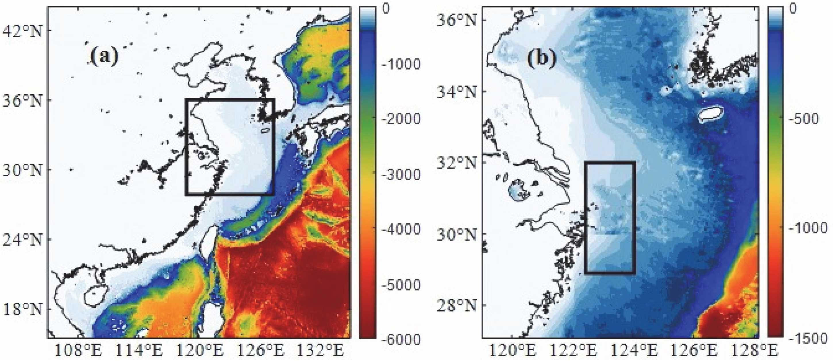
2.1. Model and Data

The regional ocean modeling system (ROMS) solves the hydrostatic, primitive equations with horizontal curvilinear coordinates and terrain-following vertical coordinate [14] and has been used to investigate regional ocean dynamics and to conduct real-time forecasting for many coastal regions successfully, such as California [15] and the Alaska coastal region [14]. The biogeochemical model, which is based on the carbon, silicon and nitrogen ecosystem (CoSiNE) model [16,17,18,19,20], is used to simulate the ecosystem dynamics of equatorial Pacific and South China successfully.

In the study, a two-level nested physical–biogeochemical coupled model (ROMS-CoSiNE) is used to simulate the chlorophyll concentration over the Yangtze River estuary. The outer model domain (L0, Figure 1a) covers the whole Chinese coastal and western Pacific region from 15.5° N to 44° N, 105° E to 135° E with a 9-km horizontal resolution. The inner one (L1, Figure 1b) covers the Yangtze River estuary and East China Sea with a 3-km horizontal resolution. There are 16 levels in the vertical direction. In this study, we only present the result from the L1 domain for its high horizontal resolution (Figure 1b), and we focus on the area of 29° N–32° N and 122.5° E–124° E (red rectangle in Figure 1b) over the Yangtze River estuary which includes the Zhoushan islands. The time period we emphasize is from April to August.

The initial condition of the coupled model is the climatological temperature, salinity, nutrients (nitrate, silicate and phosphate) and dissolved oxygen from the World Ocean Atlas (WOA) 2005 [21]. The atmospheric forcing fields, such as monthly 2 m air temperature, relative humidity, 10 m wind, precipitation, short-wave radiation, long-wave radiation, are from the National Centers for Environmental Prediction/National Center for Atmospheric Research reanalysis (NCEP/NCAR) [22]. The latent, sensible heat flux and wind stress are computed by using the air temperature, relative humidity, and wind based on the bulk formula of model [23,24]. For the biogeochemical model, there are 31 biological variables.

Table 1. The initial conditions for the coupled physical–biogeochemical model for the Yangtze River estuary.

Parameter Description	Value	Data Source
Nitrate (NO3)/mmol·m−3 Silicate (Si(OH)4)/mmol·m−3 Phosphate (PO4)/mmol·m−3 Oxygen (O2)/mmol·m−3		World Ocean Atlas 2005 (WOA05) [21]
Ammonium (NH4)/mmol·m−3	0.0001 mmol·m−3	Xiu and Chai [20]
Total alkalinity (Talk)/mmol·m−3		GLODAP dataset [25]
Total CO2 (TCO2)/mmol·m−3	0.0001 mmol·m−3	Xiu and Chai [20]
Semi-labile DOC (SDOC)/mmol·m−3	surface to bottom: decreases according to a hyperbolic tangent function from 15 mmol·m−3 to 0.01 mmol·m−3.
Labile DOC (LDOC)/mmol·m−3	0–500 m: 2.0 mmol·m−3; 500 m to bottom: 0.01 mmol·m−3.
Colored labile dissolved organic carbon (CLDOC)/mmol·m−3	0.0001 mmol·m−3
Labile DON (LDON)/mmol·m−3	9.95
Semi-labile DON (SDON)/mmol·m−3	15.38
Colored semi-labile (CSDOC)/mmol·m−3	0.4
Detritus-nitrogen (DDN)/mmol·m−3	0.0001 mmol·m−3
Detritus-silicate (DDSI)/mmol·m−3	0.0001 mmol·m−3
Detritus-carbon (DDC)/mmol·m−3	0.0001 mmol·m−3
Bacteria nitrogen (BAC)/mmol·m−3	surface to bottom: decreases according to a hyperbolic tangent function from 0.03 mmol·m−3 to 0.01 mmol·m−3.
Small phytoplankton (S1)/mmol·m−3	0.0001 mmol·m−3
Diatoms (S2)/mmol·m−3	0.0001 mmol·m−3
Coccolithophorids (S3)/mmol·m−3	0.0001 mmol·m−3
Chlorophyll in small phytoplankton (chl1)/mg·m−3	0.0001 mg·m−3
Chlorophyll in large phytoplankton (chl2)/mg·m−3	0.0001 mg·m−3
Coccolithophorids chlorophyll (chl3)/mg·m−3	0.0001 mg·m−3
Carbon in small phytoplankton (C1)/mmol·m−3	0.0001 mmol·m−3
Carbon in large phytoplankton (C2)/mmol·m−3	0.0001 mmol·m−3
Coccolithophorids carbon (C3)/mmol·m−3	0.0001 mmol·m−3
Micro zooplankton (ZZ1)/mmol·m−3	0.0001 mmol·m−3
Meso zooplankton (ZZ2)/mmol·m−3	0.0001 mmol·m−3
zz1-carbon (ZZC1)/mmol·m−3	0.0001 mmol·m−3
zz2-carbon (ZZC2)/mmol·m−3	0.0001 mmol·m−3
Particulate inorganic carbon (DDCA)/mmol·m−3	0.0001 mmol·m−3

shows all the initial conditions for ecosystem variables, and can also be found in Xiu and Chai [20].

The coupled model is also forced by freshwater discharge from the Yangtze River. The discharge of Yangtze River is based on daily observation from Datong hydrological station. The Yangtze River Datong hydrological station is located in the Meilong town of Chizhou, Anhui province. The station was built in the early twentieth century and is located at the upper boundary of the ocean tidal influence. This station has long-term discharge observation in the lower reaches of the Yangtze River. For the discharge data, we selected data from 1998 to 2010.

The observational monthly chlorophyll concentration (1998–2010) of the sea-viewing wide field-of-view sensor (SeaWiFS) is from the National Aeronautics and Space Administration (NASA) Goddard Space Flight Center (GSFC) and can be downloaded from https://oceancolor.gsfc.nasa.gov/l3/order/ (accessed on 21 August 2022). The SST data assimilation product (1998–2010) is from Estimating the Circulation and Climate of the Ocean Phase II (ECCO2). ECCO2 is an ocean reanalysis product that assimilates many types of observational data, including sea surface height, sea surface temperature, sea surface salinity from satellite missions, and in situ temperature and salinity profiles [26,27,28]. It can be download from http://apdrc.soest.hawaii.edu/data/data.php (accessed on 21 August 2022).

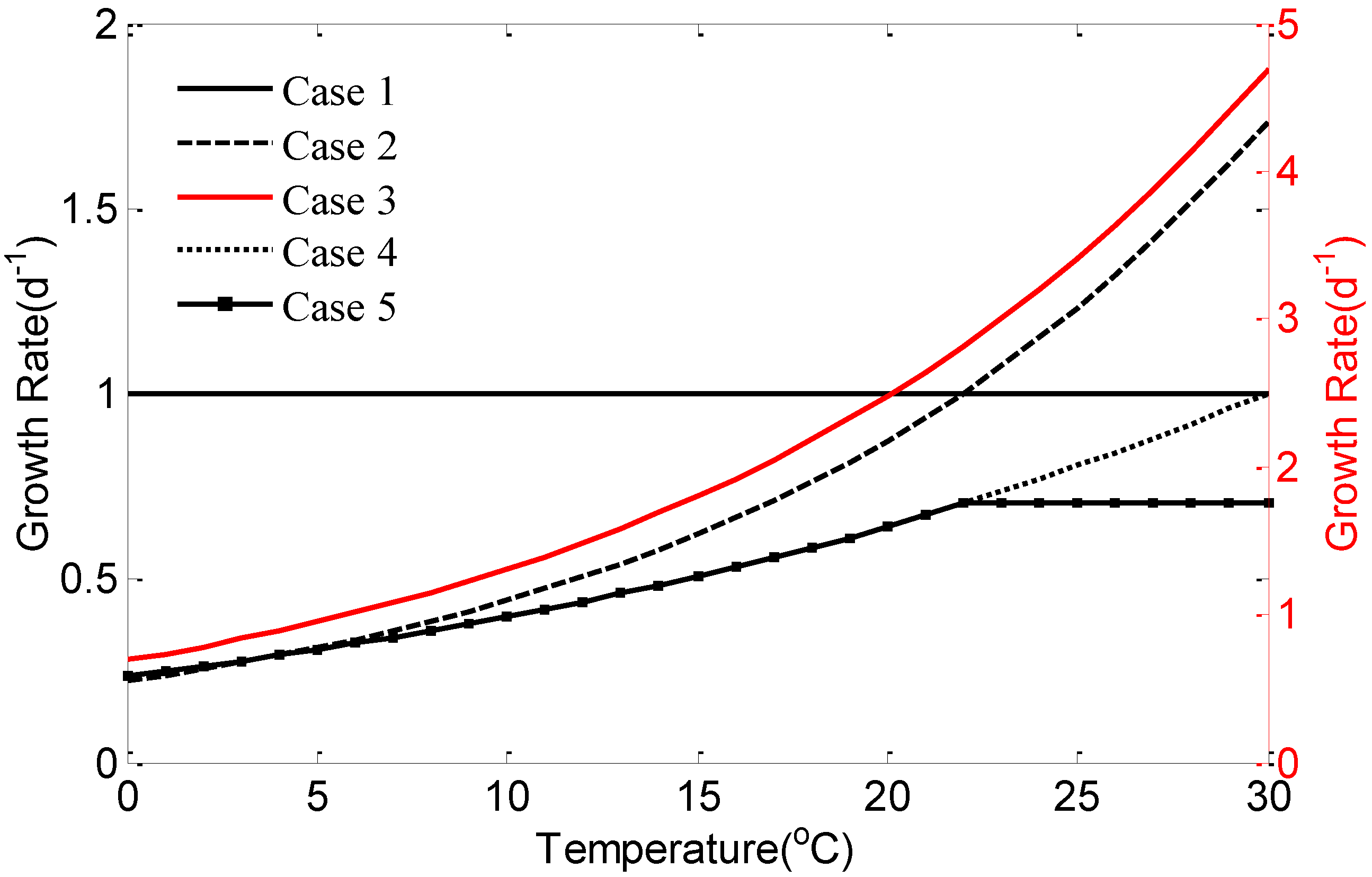
2.2. Experiment Design

In present study, the attenuation of photosynthetically active radiation is calculated based on water depth and phytoplankton biomass (Equation (1), P1: picoplankton nitrogen, P2: diatoms nitrogen, P3: coccolithophorids nitrogen), which is commonly used in most ecosystem models [20,29],

$$\mathrm{PAR}\left(\mathrm{z}\right)=\mathrm{PAR}\left(0\right)\times \exp \left\{-k_{1}z-k_2{{\displaystyle \int }}_{-z}^0\left(P1+P2+P3\right)dz\right\},$$

(1)

where $k_1$ and $k_2$ are the light attenuation coefficients of seawater (0.046 ${\mathrm{m}}^{-1}$) and phytoplankton (0.03 ${\mathrm{m}}^{-1}$), respectively.

Yangtze River freshwater discharge brings a huge amount of nutrients into the estuary [30,31,32,33,34]. Nutrients are an important factor influencing marine ecosystems, and directly affect biological processes in the ocean [34,35,36,37]. In order to study the ecological environment over the Yangtze River estuary, we first add the freshwater over the Yangtze River estuary in the physical–biogeochemical coupled model. The freshwater discharge (unit: m³/s) of the Yangtze River is first converted into a Gaussian distributed precipitation rate (unit: m/s) around the river mouth based on a spatial scale, which is a parameter related with model resolution and taken as 120 km (60 km for L1 domain) in our study. This method was used in many other studies in which the complex estuary dynamics cannot be explicitly resolved in coarse resolution ocean models [38,39,40,41]. Then, different nutrients are added in the physical–biogeochemical model, by multiplying the discharge with the observed nutrients concentration (nitrate: 41.9 mmol/m³ average from January 1963 to December 1999; silicate: 95.6 mmol/m³, and phosphate: 0.21 mmol/m³ average from January 1963 to December 1984; Liu et al. [31]), and assuming the added nutrients will be mixed in the top 10 m of the water column. In this way, we can convert the river discharge into the change of nutrient concentration rate (unit: mmol/m³·s).

The chlorophyll production in our physical–biogeochemical model can be written as the right side of Equation (2), in which the ${\mathsf{\rho }}_{\mathrm{chlorophyll}}$ is the regulation factor for chlorophyll synthesis governed by the imbalance between rates of light absorption and photosynthesis as expressed in Equation (3). NP and RP are new production and regenerated production depending on nutrients (nitrate and ammonium), light, temperature, and C (carbon): N (nitrate) ratio. ${\mathrm{P}}^{\mathrm{C}}$ (Equation (4)) is the carbon-specific photosynthetic rate, and related with the specific growth rate of phytoplankton equation ($\mathsf{\mu }$) and photosynthetically active radiation (PAR). The ${\mathsf{\theta }}_{\max }^{\mathrm{N}}$ is the maximum ratio of chlorophyll and nitrate. The ${\mathsf{\theta }}^{\mathrm{C}}$ is the ratio of chlorophyll and carbon. Coefficient $\mathsf{\alpha }$ is constant, which is taken as 0.25 in our model setup. The details of the functions and the values of relevant parameters can be found in Xiu and Chai [19,20]. Due to the seasonal variation of temperature, the specific growth rate of phytoplankton equation can directly affect the growth of phytoplankton, and is crucial for the seasonal variation of chlorophyll concentration,

$$chlorophyll\left(z\right)={\rho }_{\mathrm{chlorophyll}}\left(z\right)\left(NP\left(z\right)+RP\left(z\right)\right),$$

(2)

$${\rho }_{\mathrm{chlorophyll}}\left(z\right)=\frac{P^C\times {\theta }_{\max }^N}{\alpha \times {\theta }^C\left(z\right)\times PAR\left(z\right)},$$

(3)

$$P^C\left(z\right)=\mu \times \left(1-\mathit{exp}\left(\frac{-\alpha \times {\theta }^C\left(z\right)\times PAR\left(z\right)}{\mu }\right)\right).$$

(4)

In order to analyze the sensitivity of the chlorophyll concentration on temperature in the coupled model, five forms of the specific growth rate of phytoplankton equation were tested (

Table 2. Five kinds of the specific growth rate of phytoplankton equations in the coupled model (${\mathrm{T}}_{\mathrm{opt}}$ = 22 °C).

Cases	Specific Growth Rate of Phytoplankton Equations	Source
Case 1	Q10 = ${\mu }_0$·1.0	Eppley [6]
Case 2	$\mu$ = ${\mu }_0$·e(0.069·(T-Topt))	Zhou et al. [29]
Case 3	$\mu$ = ${\mu }_0$·0.69·(1.066T)	Eppley [6]
Case 4	$\mu$ = ${\mu }_0$·e(−4000.0·(1.0/(T+273.15)−1.0/303.15))	Geider [43]; Moore et al. [44]; Fujii et al. [45]
Case 5	$\mu$ = ${\mu }_0$·e(−4000.0·(1.0/(T+273.15)−1.0/303.15)) $\mu$= ${\mu }_0$·e(−4000.0·(1.0/(Topt+273.15)−1.0/303.15)) (T > 22 °C)	Lin [47]; Li [48]

). The forcing and boundary conditions are identical for the five experiments except different forms of specific growth rate of phytoplankton equation are used. The length of the integration is 13 years from 1998 to 2010. For the convenience of discussion, these five forms are called Case 1, Case 2, Case 3, Case 4, and Case 5, respectively. Based on the laboratory growth rate measurement, Eppley [6] suggested that the equation between temperature and growth rate should be a constant, called Q10, and the value of the Q10 is normally taken as 1.88 with the temperature in the range of 0–40 °C. In Case 1, we used Q10 = ${\mathsf{\mu }}_0$·1.0 in Chinese coastal water which has averaged a temperature of approximately 8.0–29.6 °C [42] (observation data from Ministry of Natural Resources of the People’s Republic of China, and can be download from http://www.oceanguide.org.cn/hyyj/, accessed on 21 August 2022) over the Yangtze River estuary. In Case 2, we used a form of specific growth rate of phytoplankton equation that was tested in a simplified version of the physical–biogeochemical with 13 ecological variables [29]. In Case 3, the specific growth rate of phytoplankton equation changes with temperature as ${\mathsf{\mu }}_0$·0.69·(1.066 T) [6]. The specific growth rate of phytoplankton equation of Case 4 is an exponential equation, which is commonly used in many studies [43,44,45]. Case 5 used a modified version of specific growth rate of phytoplankton equation of Case 4, based on the assumption that the phytoplankton has an optimal temperature [46] (${\mathrm{T}}_{\mathrm{opt}}$ = 22 °C) of growth [47,48]. Above the optimal temperature, phytoplankton growth decreases due to inactivation or denaturation of proteins or other factors [49]. In all the five cases, the ${\mathsf{\mu }}_0$ is 1.0 in five equations. The SST from the five numerical experiments is compared with ECCO2 product. The seasonal variability of surface chlorophyll concentration is validated against observation from SeaWiFS.

Figure 2 shows the variations of five different specific growth rate of phytoplankton equations with different temperatures. In Case 1, the growth rate is independent of temperature, and is suitable for the growth of photosynthetic unicellular algae below 40 °C. The growth rate in Case 2 gradually increases from 0 to 2.0 d⁻¹, but it changes from 0 to 5.0 d⁻¹ for Case 3, when temperature changes from 0 to 30 °C. Case 2 and Case 3 are used to estimate the growth of picoplankton and diatoms. The growth rate of Case 4 and Case 5 specific growth rate of phytoplankton equations gradually increase from 0 to 1.0 d⁻¹, when temperature changes from 0 to 30 °C. The difference between the Case 4 and Case 5 is that when temperature exceeds 22 °C, the growth rate of Case 5 is a constant and does not increase with the increase of temperature [47,48]. Rates of growth given by Case 1–3 are much higher than Case 4–5.

3. Results

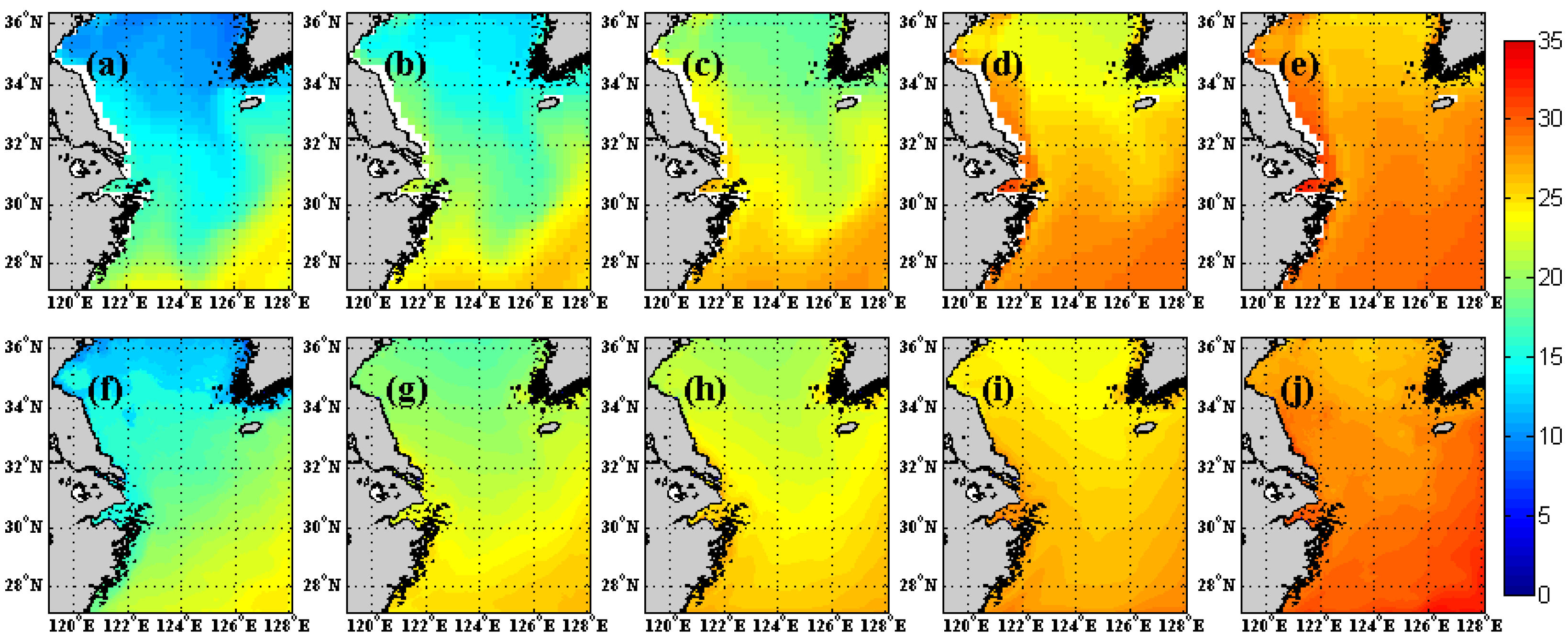
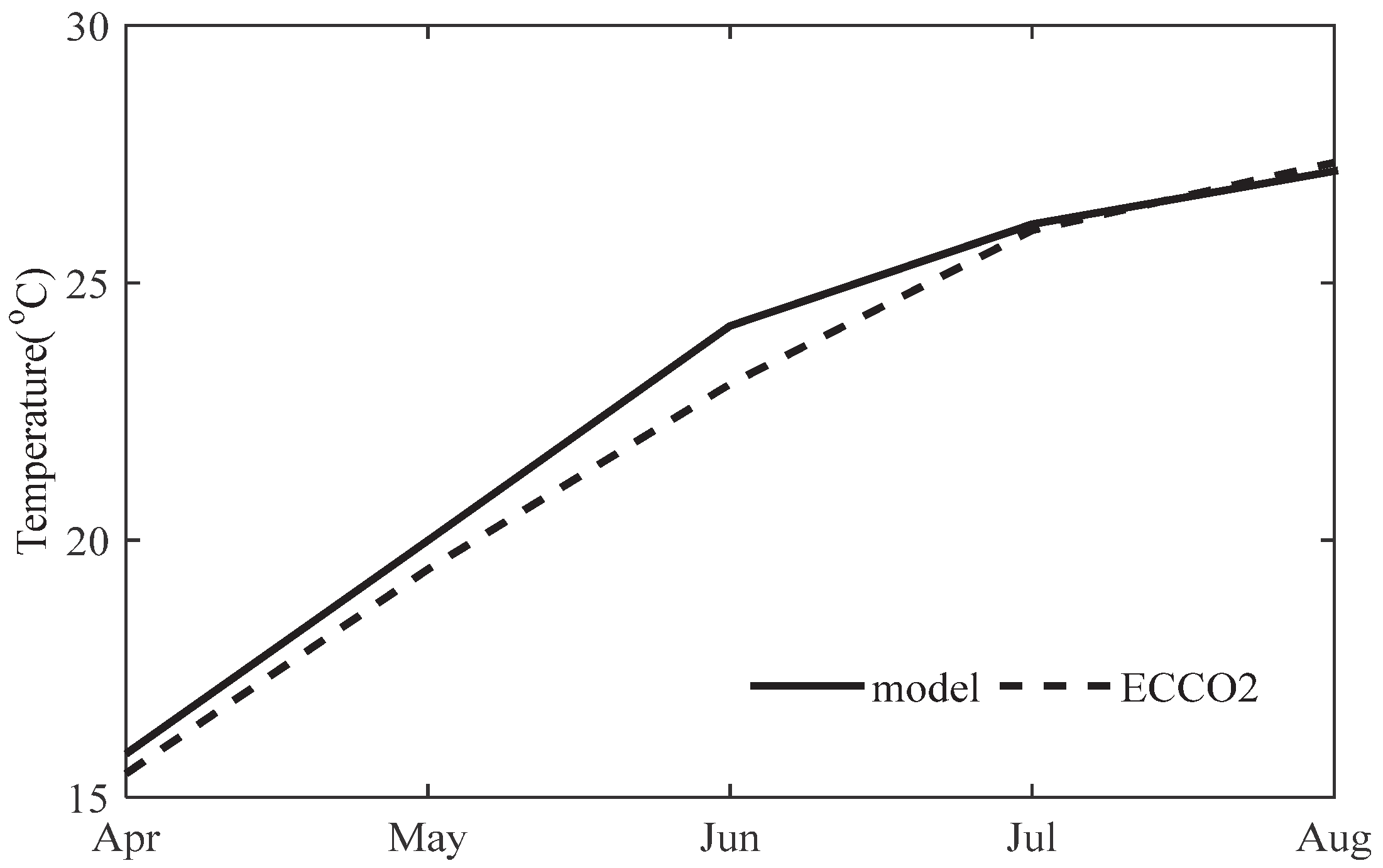
3.1. Comparison of SST with ECCO2 SST Product

In our model, the effect of temperature on the growth of phytoplankton is mainly realized through the specific growth rate of phytoplankton equation, and for different sea areas, especially in nearshore areas, affected by climate change and hydrological conditions, different specific growth rate of phytoplankton equations including temperature have different simulation results for chlorophyll concentration. In order to analyze the influence of specific growth rate of phytoplankton equation on seasonal variation of sea surface chlorophyll concentration over the region, we compared the SST from the ECCO2 product with model results from 1998 to 2010 (Figure 3). The SST fields from five cases are the same because identical heat flux forcing fields are used for all five experiments. Thus, the Case 5 result is chosen to compare with ECCO2. Based on the ECCO2 product (Figure 3a–e), SST gradually increases from 15 °C to 30 °C from April to August (13-year average from 1998–2010) over the Yangtze River estuary. The SST from model (Figure 3f–j) and ECCO2 are highly consistent.

In addition to the spatial pattern, we also compare the time series of SST from model and ECCO2 averaged over 29° N–32° N, 122.5° E–124° E, which is a region where harmful algal bloom events happen frequently [47,50]. The model and ECCO2 (Figure 4) both show the gradual increase of SST from April to August, whereas the model tends to overestimate SST by about 1 °C from April to June. Note that the temperature around the Yangtze River estuary is above 22 °C for the month of June to August, and the specific growth rate of phytoplankton equation of Case 5 will reach a maximum at 22 °C and keep as a constant for higher temperature. Thus, the model can reproduce the spatial pattern and seasonal variability of SST around the Yangtze River estuary.

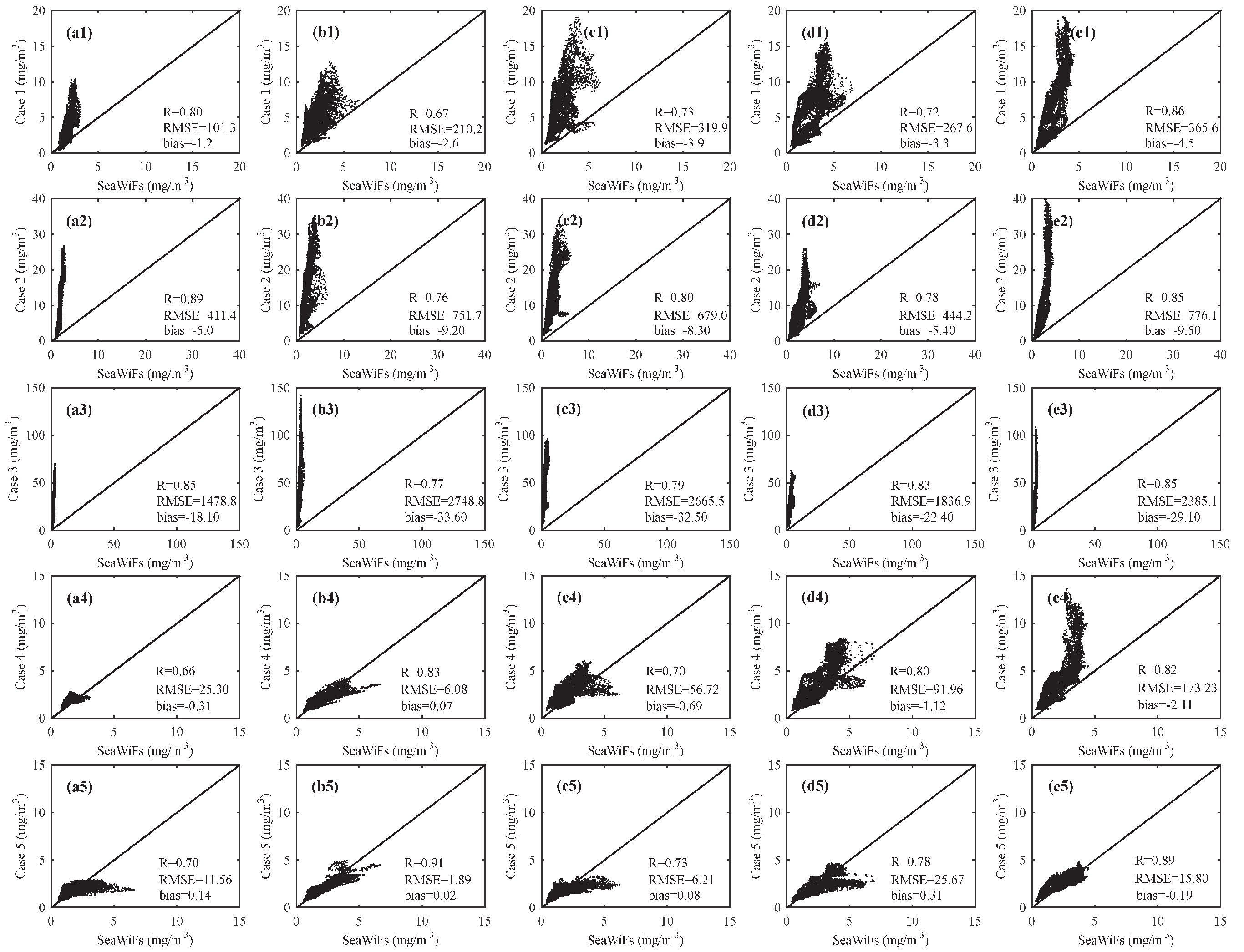
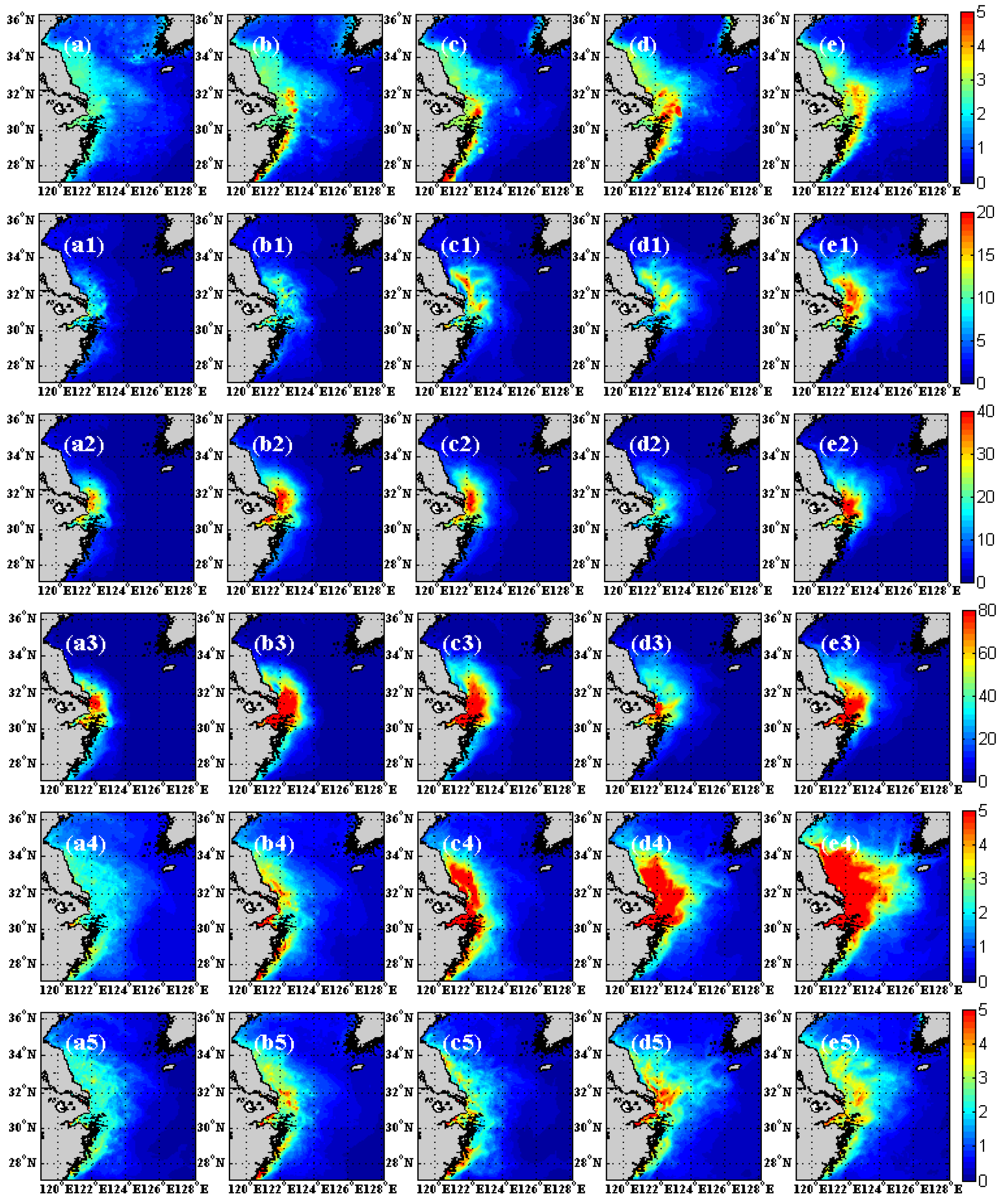
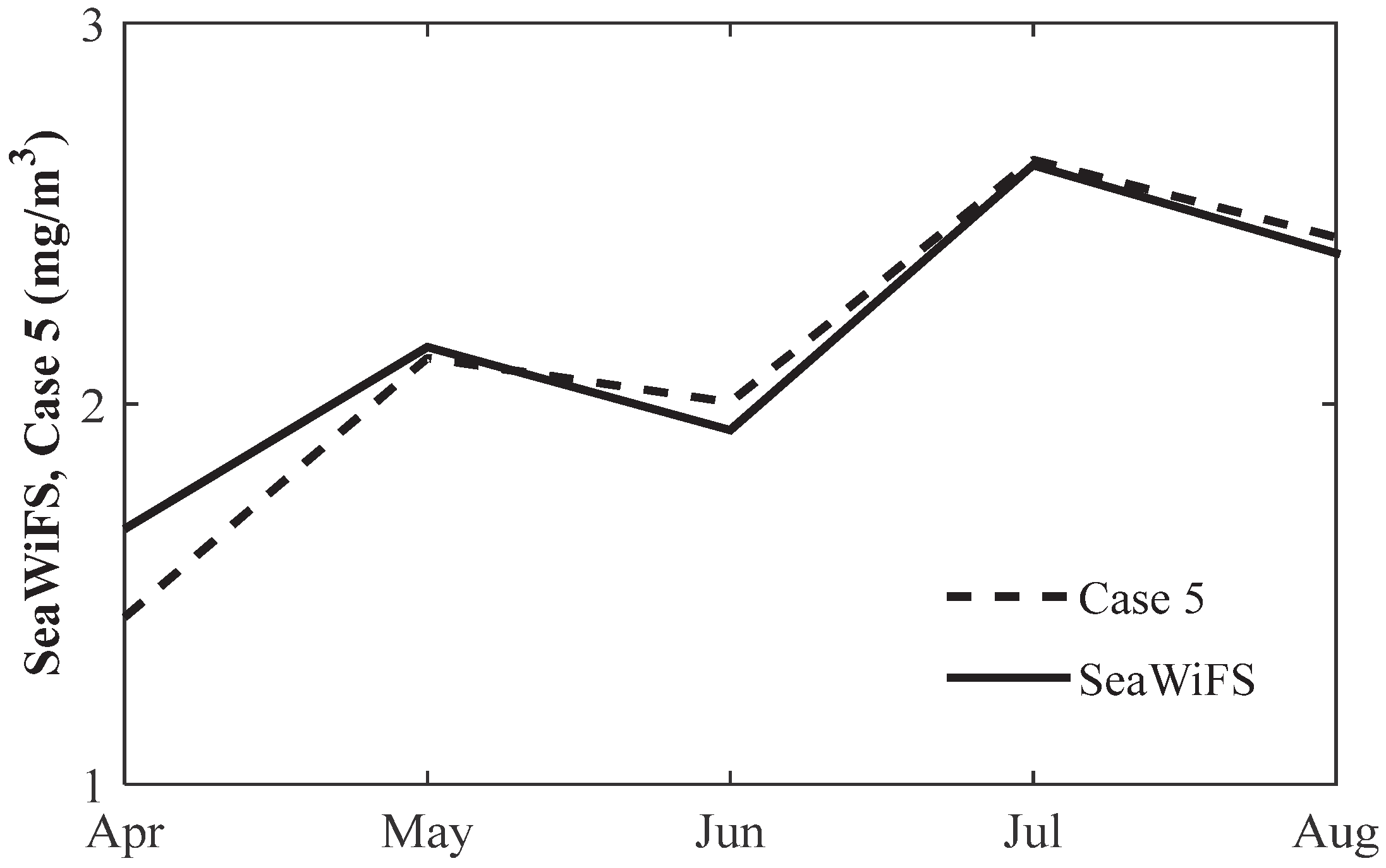
3.2. Comparison of Chlorophyll with Observation

Because most of the harmful algal bloom events occur during spring and summer over the Yangtze River estuary [13,51], we focus on the validation of chlorophyll during this time period. The chlorophyll from model results (5 Cases) are used to validate against chlorophyll from SeaWiFS over the Yangtze River estuary. The scatter plot can well reflect the linear relationship between the two variables. The scatter plot of Figure 5a1–e1 show the validations of Case 1 and SeaWiFS from April to August, and the validations of Case 2 and SeaWiFS are shown in Figure 5a2–e2, and so on. The RMSEs between chlorophyll of SeaWiFS and Case 5 from April to August averaged from 1998 to 2010 are all below 25.67 mg/m³, with the bias of varying from −0.19 mg/m³ to 0.31 mg/m³, and the correlation coefficients are all above 0.7. The comparison between Case 5 and SeaWiFS is better than the comparisons between Case 1–4 and SeaWiFS. From the above comparisons, we find that Cases 1–4 are all overestimated chlorophyll, and Case 5 is the closest to SeaWiFS.

Although there is large bias between the model and SeaWiFS, it is encouraging to note the similarity between chlorophyll concentration spatial distribution from the model (Figure 6a1–e5) and SeaWiFS (Figure 6a–e). The spatial distribution of averaged chlorophyll concentration from SeaWiFS is characterized by high value ranging from 0 to 5 mg/m³ over the near shore, and it gradually decreases to low value in the open sea. In terms of temporal evolution, chlorophyll concentration increases from April to July, and decreases in August over the region of 29° N–32° N, 122.5° E–124° E. The region of high chlorophyll concentration (higher than 5 mg/m³) extends northeastward gradually from April to July, and is caused by freshwater discharge, especially in the region of 29° N–32° N, 122.5° E–124° E [52,53]. Although there exist large differences in the magnitude of chlorophyll concentration between Cases 1–3 and SeaWiFS, the spatial distributions of Cases 1–3 all have high values near the shore and low values offshore (Figure a1–e3). For Case 4, the chlorophyll concentration ranging in 0–10 mg/m³, and the value gradually increases from April to August. Case 5 shows the same spatial distribution to SeaWiFS, and the magnitude of concentration is also from 0 to 5 mg/m³. However, the chlorophyll concentration of Case 5 is significantly lower than Case 4 from June to August, which may be related to the fact that the SST exceeded the optimal temperature of phytoplankton growth of 22 °C. The above analysis shows that the model which uses the fifth specific growth rate of phytoplankton equation can reproduce the spatial distribution of chlorophyll on seasonal timescales over the Yangtze River estuary.

We also compared the time series of seasonal variation of chlorophyll concentration from SeaWiFS with the model result (13-year average from 1998–2010). Figure 7 shows the time series of monthly chlorophyll concentration from SeaWiFS and simulation results by using the fifth specific growth rate of phytoplankton equation from April to August. We note that both SeaWiFS and Case 5 show two peaks from April to August, and their values are very close. The above analysis indicated that the model can reproduce the seasonal evolution of chlorophyll concentration.

4. Discussion and Conclusions

In the physical–biogeochemical coupled model, different forms of specific growth rate of phytoplankton equation are used in earlier research papers for various regional oceans. In this study, five commonly used forms of specific growth rate of the phytoplankton equation are tested in a physical–biogeochemical coupled model for the Yangtze River estuary. These five forms of specific growth rate of phytoplankton equations vary from independent of temperature (Case 1), exponentially increasing with temperature (Cases 2, 3, and 4), to increasing to an optimal temperature for which the phytoplankton growth rate reaches a maximum and then stays as a constant with further increases in temperature (Case 5). The rates of growth given by Cases 1–3 are much higher than Cases 4–5, so that the chlorophyll concentration of Cases 1–3 are higher than that of Cases 4–5. Model results are compared against ECCO2 SST and satellite chlorophyll observations from the SeaWiFS instrument. The results show that the model can reproduce the spatial distribution of SST. The chlorophyll concentration using the specific growth rate of phytoplankton equation of Case 5 bears great similarity to the chlorophyll concentration from SeaWiFS in terms of spatial distribution and temporal evolution at seasonal time scale and might be suitable for current physical–biogeochemical model of the Yangtze River estuary.

However, how do we know the growth rate of phytoplankton will remain at the maximum when SST is higher than 22 °C? The selection of 22 °C as the optimal temperature for the growth of phytoplankton is based on Li [47] and Lin [48]. Li used a three-dimensional ecosystem model to test the effect of temperature on dinoflagellates and diatoms over the Yangtze River estuary, and showed that when the temperature is 20 °C, the area and cumulative occurrence time of dinoflagellates’ red tide were the largest. When the temperature is 20–24 °C, the scale of diatom red tide increased with the increase of temperature. Lin recognized that the area of highly stratified diluted water with temperature higher than 22 °C around Yangtze River estuary is also the region with high chlorophyll concentration, salinity lower than 30 psu, and surface turbidity around 1–3 ntu.

There are three kinds of phytoplankton in our biological model, macrophytoplankton, diatoms, and coccolithophorids. The chlorophyll concentration is derived according to the amount of three kinds of phytoplankton, and the three kinds of phytoplankton share the same specific growth rate of phytoplankton equation in the physical–biogeochemical coupled model [19,20]. When 22 °C is set as the optimum temperature, the chlorophyll concentration and spatial distribution are the closest to the observation. Thus, the fifth specific growth rate of phytoplankton equation is selected for the Yangtze River estuary in our physical–biogeochemical coupled model. When the structure of the biological model and region of interest are different, the optimal temperature may need further adjustment.

References

1. Hallegraeff, G.M. Ocean climate change, phytoplankton community responses, and harmful algal blooms: A formidable predictive challenge. J. Phycol. 2010, 46, 220–235. [Google Scholar] [CrossRef]
2. Agawin, N.; Duarte, C.M.; Agusti, S. Nutrient and temperature control of the contribution of picoplankton to phytoplankton biomass and production. Limnol. Oceanogr. 2000, 45, 591–600. [Google Scholar] [CrossRef]
3. Zinser, E.R.; Johnson, Z.I.; Coe, A. Influence of light and temperature on Prochlorococcus ecotype distributions in the Atlantic Ocean. Limnol. Oceanogr. 2007, 52, 2205–2220. [Google Scholar] [CrossRef]
4. Di Toro, D.M.; Connor, D.J.; Thomann, R.V. A dynamic model of the phytoplankton population in the Sacramento-San Joaquin Delta. Adv. Chem. 1971, 106, 131–180. [Google Scholar]
5. Mclaren, I.A. Effects of temperature on growth of zooplankton, and the adaptive value of vertical migration. J. Fish. Res. Board Can. 1963, 20, 685–727. [Google Scholar] [CrossRef]
6. Eppley, R.W. Temperature and phytoplankton growth in the sea. Fish. Bull. 1972, 70, 1063–1085. [Google Scholar]
7. Goldman, J.G.; Carpenter, E.J. A kinetic approach to the effect of temperature on algal growth. Limnol. Oceanogr. 1974, 19, 756–766. [Google Scholar] [CrossRef]
8. Brush, M.; Brawley, J.W.; Nixon, S.W. Modeling phytoplankton production: Problems with the Eppley curve and an empirical alternative. Mar. Ecol. Prog. Ser. 2002, 238, 31–45. [Google Scholar] [CrossRef] [Green Version]
9. Bissinger, J.E.; Montagnes, D.J.S.; Sharples, J. Predicting marine phytoplankton maximum growth rates from temperature: Improving on the Eppley curve using quantile regression. Limnol. Oceanogr. 2008, 53, 487–493. [Google Scholar] [CrossRef] [Green Version]
10. Moisan, J.R.; Moisan, T.A.; Abbott, M.R. Modelling the effect of temperature on the maximum growth rates of phytoplankton populations. Ecol. Modell. 2002, 153, 197–215. [Google Scholar] [CrossRef]
11. Deng, J.; Huang, L.W.; Wu, G.X.; Yu, R.C. 3D fine resolution modeling of China yellow east sea’s circulation with complete forcing in winter. J. Wuhan Univ. Technol. 2003, 2, 161–165. [Google Scholar]
12. Liu, X.Q.; Yin, B.S.; Hou, Y.J. The dynamic of circulation and temperature-salinity structure in the Changjiang mouth and its adjacent marine area, II Major characteristics of the circulation. Oceanol. Limnol. Sin. 2008, 4, 312–320. [Google Scholar]
13. Chen, C.S.; Zhu, J.R.; Beardsley, R.C. Physical-biological sources for dense algal blooms near the Changjiang River. Geophys. Res. Lett. 2003, 30, 1515. [Google Scholar] [CrossRef] [Green Version]
14. Shchepetkin, A.F.; McWilliams, J.C. The Regional Ocean Modeling System (ROMS): A split-explicit, free-surface, topography following coordinates ocean model. Ocean. Model. 2005, 9, 347–404. [Google Scholar] [CrossRef]
15. Lvanov, L.M.; Collins, C.A.; Marchesiello, P. One model validation for meso/submesoscale currents: Metrics and application to ROMS off Central California. Ocean. Model. 2009, 28, 209–225. [Google Scholar]
16. Chai, F.; Lindley, S.T.; Barber, R.T. Origin and maintenance of a high NO3 condition in the equatorial Pacific. Deep Sea Res. Part II 1996, 43, 1031–1064. [Google Scholar] [CrossRef]
17. Chai, F.; Dugdale, R.C.; Peng, T.H. One-dimensional ecosystem model of the equatorial Pacific upwelling system. Part I: Model development and silicon and nitrogen cycle. Deep Sea Res. Part II 2002, 49, 2713–2745. [Google Scholar] [CrossRef]
18. Xiu, P.; Chai, F. Modeled biogeochemical responses to mesoscale eddies in the South China. J. Geophys. Res. Oceans 2011, 116, C10. [Google Scholar] [CrossRef] [Green Version]
19. Xiu, P.; Chai, F. Spatial and temporal variability in phytoplankton carbon, chlorophyll, and nitrogen in the North Pacific. J. Geophys. Res. Oceans 2012, 117, C11023. [Google Scholar] [CrossRef]
20. Xiu, P.; Chai, F. Connections between physical, optical and biogeochemical processes in the Pacific Ocean. Prog. Oceanogr. 2014, 122, 30–53. [Google Scholar] [CrossRef]
21. Garcia, H.E.; Locarnini, R.A.; Boyer, T.P. World Ocean Atlas 2005, Nutrients (Phosphate, Nitrate, Silicate); Government Printing Office: Washington, DC, USA, 2006; pp. 2–14. [Google Scholar]
22. Kalnay, E.; Kanamitsu, M.; Kistler, R. The NCEP/NCAR 40-year reanalysis project. Bull. Am. Meteorol. Soc. 1996, 77, 437–471. [Google Scholar] [CrossRef]
23. Kondo, J. Air-sea bulk transfer coefficients in diabatic conditions. Bound. Layer Meteorol. 1975, 9, 91–112. [Google Scholar] [CrossRef]
24. Large, W.G.; Pond, S. Sensible and latent heat flux measurements over the ocean. J. Phys. Oceanogr. 1982, 12, 464–482. [Google Scholar] [CrossRef]
25. Key, R.M.; Kozyr, A.; Sabine, C.L. A global ocean carbon climatology: Results from GLODAP. Global Biogeochem. Cycles 2004, 18, GB4031. [Google Scholar] [CrossRef]
26. Marshall, J.C.; Adcroft, A.; Hill, C. A finite-volume, incompressible Navier Stokes model for studies of the ocean on parallel computers. J. Geophys. Res. Oceans 1997, 102, 5753–5766. [Google Scholar] [CrossRef]
27. Wunsch, C.; Heimbach, P. Practical global ocean state estimation. Phys. D Nonlinear Phenom. 2007, 230, 197–208. [Google Scholar] [CrossRef]
28. Wunsch, C.; Heimbach, P.; Ponte, R.M. The global general circulation of the ocean estimated by the ECCO-Consortium. Oceanography 2009, 22, 88–103. [Google Scholar] [CrossRef]
29. Zhou, F.; Chai, F.; Huang, D.J. Investigation of hypoxia off the Changjiang Estuary using a coupled model of ROMS-CoSiNE. Prog. Oceanogr. 2017, 159, 237–254. [Google Scholar] [CrossRef]
30. Zhang, J. Nutrient elements in large Chinese estuaries. Cont. Shelf Res. 1996, 16, 1023–1045. [Google Scholar] [CrossRef]
31. Liu, X.C.; Shen, H.T.; Huang, Q.H. Concentration variation and flux estimation of dissolved inorganic nutrient from the Changjiang River into its estuary. Oceanol. Limnol. Sin. 2002, 33, 332–340. [Google Scholar]
32. Shen, Z.L.; Liu, Q. Nutrients in the Changjiang River. Environ. Monit. Assess 2008, 153, 27–44. [Google Scholar] [CrossRef] [PubMed]
33. Chai, C.; Yu, Z.M.; Shen, Z.L. Nutrient characteristics in the Yangtze River Estuary and the adjacent East China Sea before and after impoundment of the Three Gorges Dam. Sci. Total Environ. 2009, 407, 4687–4695. [Google Scholar] [CrossRef] [PubMed]
34. Luo, B.Z.; Liu, R.Y. Construction of Three Gorge Dam Project and the Ecology and Environment in the Estuary Science Press; Beijing Publication: Beijing, China, 1994; p. 343. [Google Scholar]
35. Domingues, R.B.; Barbosa, A.; Galvão, H. Nutrients, light and phytoplankton succession in a temperate estuary (the Guadiana, south-western Iberia). Estuar. Coast. Shelf Sci. 2005, 64, 249–260. [Google Scholar] [CrossRef]
36. Furnas, M.; Mitchell, A.; Skuza, M. In the other 90%: Phytoplankton responses to enhanced nutrient availability in the Great Barrier Reef Lagoon. Mar. Pollut. Bull. 2005, 51, 253–265. [Google Scholar] [CrossRef] [PubMed]
37. Paerl, H.W. Assessing and managing nutrient-enhanced eutrophication in estuarine and coastal waters: Interactive effects of human and climatic perturbations. Ecol. Eng. 2006, 26, 40–54. [Google Scholar] [CrossRef]
38. Wang, X.C.; Chao, Y.; Zhang, H.C. Modeling tides and their influence on the circulation in Prince William Sound, Alaska. Cont. Shelf Res. 2013, 63, S126–S137. [Google Scholar] [CrossRef]
39. Berdeal, I.B.; Hickey, B.M.; Kawase, M. Influence of wind stress and ambient flow on a high discharge river plume. J. Geophys. Res. Oceans 2002, 107, 3130. [Google Scholar] [CrossRef] [Green Version]
40. Jin, M.B.; Wang, J. Interannual variability and sensitivity study of the ocean circulation and thermohaline structure in Prince William Sound, Alaska. Cont. Shelf Res. 2004, 24, 393–411. [Google Scholar] [CrossRef]
41. Mooers, C.N.K.; Wu, X.L.; Bang, I. Performance of a nowcast/forcast system for Prince William Sound, Alaska. Cont. Shelf Res. 2007, 29, 42–60. [Google Scholar] [CrossRef]
42. Gong, C.G.; Wen, Y.H.; Wang, B.W. Seasonal variation of chlorophyll a concentration, primary production and environmental conditions in the subtropical East China Sea. Deep Sea Res. Part II 2003, 50, 1219–1236. [Google Scholar] [CrossRef]
43. Geider, R.J.; MacIntyre, H.L.; Kana, T.M. A dynamic regulatory model of phytoplanktonic acclimation to light, nutrients, and temperature. Limnol. Oceanogr. 1998, 43, 679–694. [Google Scholar] [CrossRef]
44. Moore, J.K.; Doney, S.C.; Kleypas, J.A. An intermediate complexity marine ecosystem model for the global domain. Deep Sea Res. 2002, 49, 403–462. [Google Scholar] [CrossRef] [Green Version]
45. Fujii, M.; Boss, E.; Chai, F. The value of adding optics to ecosystem models: A case study. Biogeosciences 2007, 4, 817–835. [Google Scholar] [CrossRef] [Green Version]
46. Li, W.K.W. Temperature Adaptation in Phytoplankton: Cellular and Photosynthetic Characteristics. Environ. Sci. Res. 1980, 19, 259–279. [Google Scholar]
47. Li, Y.B. The Study of the Seasonal Occurrence Mechanism of HABs in the Changjiang Estuary and Its Adjacent Sea. Ph.D. Dissertation, Ocean University of China, Qingdao, China, 2008; pp. 68–70. [Google Scholar]
48. Lin, J. A Modeling Study of the Phytoplankton Dynamics off the Changjiang Estuary. Ph.D. Dissertation, East China Normal University, Shanghai, China, 2011; pp. 38–39. [Google Scholar]
49. Ratkowsky, D.A.; Lowry, R.K.; McMeekin, T.A. Model for bacterial culture growth rate throughout the entire biokinetic temperature range. J. Bacteriol. Res. 1983, 154, 1222–1226. [Google Scholar] [CrossRef] [Green Version]
50. Zhou, M.J.; Yan, T.; Zou, J.Z. Preliminary analysis of the characteristics of red tide areas in Changjiang River Estuary and its adjacent sea. Chin. J. Appl. Ecol. 2003, 14, 1031–1038. [Google Scholar]
51. Ye, S.F.; Ji, H.H.; Cao, L. Red tides in the Yangtze River Estuary and adjacent sea areas: Causes and mitigation. Mar. Sci. 2002, 28, 26–32. [Google Scholar]
52. Chen, L.Y.L.; Chen, H.Y.; Gong, G.C. Phytoplankton production during a summer coastal upwelling in the East China Sea. Cont. Shelf Res. 2004, 24, 1321–1338. [Google Scholar] [CrossRef]
53. Wang, Y.; Jiang, H.; Jin, J.X. Spatial-Temporal variations of chlorophyll in the adjacent sea area of the Yangtze River estuary influenced by Yangtze River Discharge. Int. J. Environ. Res. Public Health 2015, 12, 5420–5438. [Google Scholar] [CrossRef]
Figure 1. (a) The outer model domain covers the whole Chinese coastal region and part of western Pacific. The range of the black rectangle is the inner one (27° N–36° N, 119° E–128° E). (b) The inner model domain covers the Yangtze River estuary and part of East China Sea. The black rectangle (29° N–32° N, 122.5° E–124° E) is the area we analyzed.
Atmosphere 13 01748 g001
Figure 2. Growth rate changes with temperature for five forms of specific growth rate of phytoplankton equation, Case 1 to 5.
Atmosphere 13 01748 g002
Figure 3. Monthly SST of ECCO2 from April to August (13-year average from 1998–2010) of Yangtze River estuary (ae, top row). The (fj) are the same as (ae), but for the model results.
Atmosphere 13 01748 g003
Figure 4. The seasonal cycle of ECCO2 SST and model result from April to August averaged over 29° N–32° N, 122.5° E–124° E from 1998 to 2010.
Atmosphere 13 01748 g004
Figure 5. Comparisons of chlorophyll from model (five cases) against SeaWiFS from April to August (13-year average from 1998–2010) within the area of 29° N–32° N and 122.5° E–124° E. The figures in the first row (a1e1) are for Case 1 and SeaWiFS. The figures in the second row (a2e2) are from Case 2 and SeaWiFS. The figures in the third row (a3e3) are from Case 3 and SeaWiFS. The figures in the fourth row (a4e4) are from Case 4 and SeaWiFS. The figures in the fifth row (a5e5) are from Case 5 and SeaWiFS. The correlation coefficient (R), root mean square error (RMSE) and bias between model and SeaWiFS are shown in each figure.
Atmosphere 13 01748 g005
Figure 6. Monthly chlorophyll concentration of SeaWiFS from April to August (13-year average from 1998–2010) of Yangtze River estuary (ae, top row). The (a1e5) are the same as (ae), but for the model results (five cases). The figures in the second row (a1e1) are for Case 1. The figures in the third row (a2e2) are from Case 2. The figures in the fourth row (a3e3) are from Case 3. The figures in the fifth row (a4e4) are from Case 4. The figures in the sixth row (a5e5) are from Case 5.
Atmosphere 13 01748 g006
Figure 7. The seasonal cycle of 1998–2010 averaged chlorophyll concentration from SeaWiFS and model result (Case 5) over 29° N–32° N, 122.5° E–124° E.
Atmosphere 13 01748 g007