Variation of Runoff and Runoff Components of the Lhasa River Basin in the Qinghai-Tibet Plateau under Climate Change

Abstract

Quantitative analysis of changes in Lhasa River runoff components was significant to local water resources management. This study constructed the spatial processes in hydrology (SPHY) model in the Lhasa River Basin and optimized the model’s parameters using the hydrograph partitioning curves (HPC) method. The Lhasa River Basin’s precipitation and temperature were forecasted for 2020 to 2100 using the statistical downscaling model (SDSM) and two scenarios from the fifth generation of the Canadian earth system model (CanESM5) dataset, shared socioeconomic pathways 1-2.6 (SSP1-2.6) and shared socioeconomic pathways 2-4.5 (SSP2-4.5). This study analyzed the potential changes in Lhasa River runoff and components based on the future climate. The results showed that the Lhasa River runoff from 2010 to 2019 was composed of snowmelt runoff, glacier melt runoff, rainfall runoff, and baseflow, with the proportions of 15.57, 6.19, 49.98, and 28.26%, respectively. From 2020 to 2100, under the SSP1-2.6 scenario, the precipitation and average temperature increased by 0.76mm and 0.08 °C per decade. Under the SSP2-4.5 scenario, the increasing rate was 3.57 mm and 0.25 °C per decade. Due to the temperature increase, snowmelt and glacier melt runoff showed a decreasing trend. The decline rate of total runoff was 0.31 m³/s per year under the SSP1-2.6 scenario due to the decrease in baseflow. Under the SSP2-4.5 scenario, total runoff and rainfall runoff showed a clear increasing trend at an average rate of 1.13 and 1.16 m³/s per year, respectively, related to the significant increase in precipitation. These conclusions suggested that climate change significantly impacted the Lhasa River’s total runoff and runoff components.

1. Introduction

Snowmelt and glacier melt runoff, the essential supply sources for rivers, are a critical element of hydrological simulation in high latitudes or alpine belts globally [1]. The Lhasa River Basin, located on the Qinghai-Tibet Plateau, is a typical alpine snow-covered and cold region with frequent polymorphic phase water transitions. The different water sources flow into the river channel through various paths on the surface and underground. As a result, the composition and formation mechanisms of runoff water sources are complex. Moreover, the response characteristics of runoff from different water sources to climate change are significantly different, challenging the research on runoff variation [2].

In order to accurately predict runoff changes under the influence of climate change in the Lhasa River Basin, it is first necessary to analyze the water source composition of runoff quantitatively. There are two main methods to analyze the composition of runoff water sources: one is the reverse analysis method based on tracer elements, and the other is the forward analysis method based on the hydrological model [3]. Based on the qualitative analysis of hydrogen and oxygen isotopes, some studies have found that the runoff water sources of the Lhasa River included rainfall, glacier meltwater, snow meltwater, and groundwater [4,5,6]. The distributed hydrological model is an essential tool for studying the hydrological process. Through the distributed simulation of the runoff process formed by different water sources, it is relatively convenient to quantitatively analyze the water source composition of the runoff [7]. Prasch et al. presented a distributed modeling approach to determine the contribution of snowmelt and glacier melt to the total runoff of the Lhasa River under past climatic conditions [8]. Research using the snowmelt runoff model (SRM) and moderate-resolution imaging spectroradiometer (MODIS) data to simulate the contribution of snow and glacier meltwater to the total runoff in the Lhasa River Basin determined it was 3–6% [1,9].

However, some general hydrological models, such as the SRM model [10] and soil and water assessment tool (SWAT) [11,12,13,14] model, cannot divide the runoff components. The spatial processes in hydrology (SPHY) [15,16] model can divide rainfall runoff, snowmelt runoff, glacier melt runoff, and baseflow from the total runoff. The SPHY model is applied to many watersheds in alpine regions, analyzing the corresponding river runoff components [16,17,18,19,20]. Using the SPHY model to study the runoff contribution of the Gilgit River, Latif et al. [20] showed that the average snowmelt contribution was 62%, followed by glacier melt at 28% and rainfall at 10%. Wu et al. [17] applied the SPHY model in the Upper Shule River, which showed that the baseflow contributed the most to the total runoff, followed by glacier melt, rainfall, and snowmelt runoff, with an average annual contribution of 38, 28, 18, and 16%, respectively. Vishal et al. [19] suggested that the contribution of glacier melt decreased from 18 to 12%, while the contribution of snowmelt increased from 58 to 64% in the Baspa River from 2000 to 2018 based on the SPHY model.

As the Third Pole in the world and the Water Tower of Asia [21,22], the Qinghai-Tibet Plateau is the highest and very sensitive to global warming [23]. As a result, river runoff changes and its composition on the Qinghai-Tibet Plateau are very susceptible to meteorological influences. From 1961 to 2001, the annual precipitation and average temperature of the Qinghai-Tibet Plateau showed an increasing trend, 0.447 °C and 6.14 mm per decade, respectively [24]. The study showed that the reference evapotranspiration on the Qinghai-Tibet Plateau decreased on average by 0.6909 mm per year from 1970 to 2009 [25]. These changes have significantly altered the land surface processes regarding glacier retreat and runoff variation of the plateau river [26,27,28,29]. Thus, the annual average runoff in the Lhasa River Basin presented an increasing trend. The changing trend in runoff was consistent with the changing temperature and precipitation. On an annual scale, the runoff was mainly affected by precipitation. On a monthly scale, summer runoff was mainly affected by precipitation, and winter runoff was mainly affected by the increase in winter temperature in the past 30 years [30].

In order to understand the variations of the future runoff and its components of the Lhasa River, it is first necessary to know the future climate change patterns of the Lhasa River Basin. Based on the coupled model intercomparison project phase 5 (CMIP5) forecast data, Liu et al. analyzed that temperature and annual precipitation would increase under future climate conditions. Evaporation, runoff, and water flow would show an increasing trend, while spring snowpack would decrease sharply [31]. Compared with CMIP5, the simulation effect of the coupled model intercomparison project Phase 6 (CMIP6) mode released in 2019 has been significantly improved [32,33,34]. Currently, the relevant research on climate change in the Lhasa River Basin using CMIP6 model data is still in its infancy. There is a lack of research on the future temporal and spatial changes in surface air temperature and precipitation in the Lhasa River Basin, represented by CMIP6 data under different scenarios [35,36].

The equifinality of different parameters of the hydrological model is a fundamental reason for the difference in the results of water source analysis. Recent research has shown that more hydrological characteristic information could be extracted from the flow time series, determining the model parameters and reducing the equifinality for different parameters [37]. He et al. [38,39] proposed the hydrograph partitioning curves (HPC) division method, which divided the flow hydrographs based on the dominant runoff and calibrated the corresponding constitutive parameters based on the subsets of flow hydrographs dominated by different water sources. The method effectively reduces the equifinality for different parameters of the hydrological model.

Therefore, this study constructed the SPHY model in the Lhasa River Basin and optimized the parameters of this model step-by-step in combination with the results of the HPC division method. This work aims to: (1) investigate the adaptability of the SPHY model in simulating the streamflow in the Lhasa River basin, (2) analyze Lhasa River runoff components and the proportion of each component, (3) simulate future temperature and precipitation in the Lhasa River Basin combining the statistical downscaling model (SDSM) and CMIP6 dataset, and (4) predict variation in runoff components under future climate conditions. The findings of this study will be helpful for future research on the Lhasa River Basin and will aid government managers in making logical plans for the Lhasa River’s water resources.

2. Materials and Methods

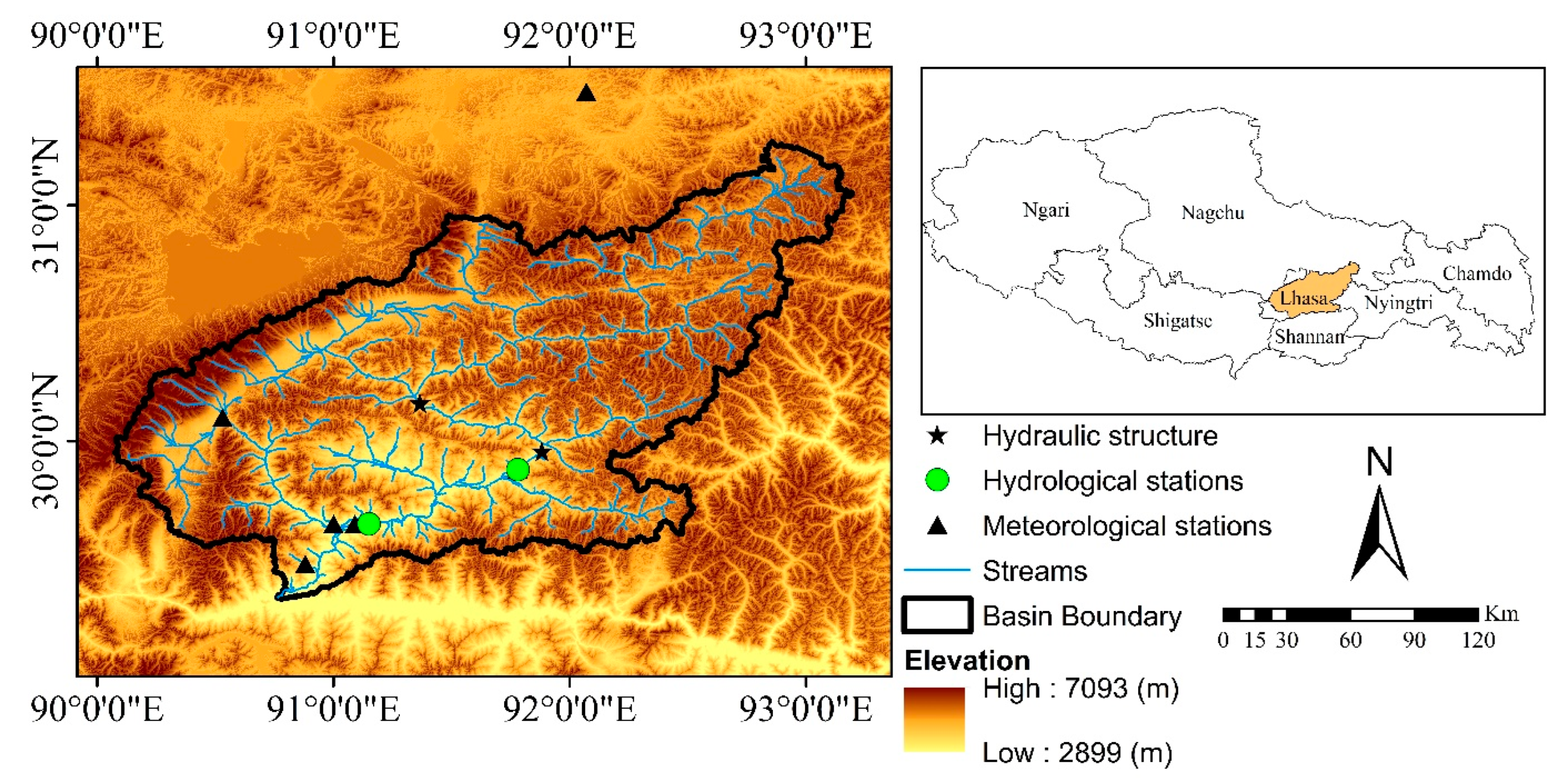
2.1. Study Areas

The Lhasa River is the main tributary on the left side of the middle reaches of the Yarlung Zangbo River. It originates from the southern foot of the middle section of the Nyainqentanglha Mountains, with an elevation range of 3580–5500 m.a.s.l. It is one of the highest braided rivers in the world. The Lhasa River Basin encompasses the region from 29°20′ N–31°15′ N to 90°05′ E–93°20′ E, with a total length of 568 km and a watershed area of 32,896 km². The climate characteristics of the Lhasa River Basin is the plateau temperate arid and semi-arid climate, and the vegetation types mainly include mountain shrub grassland and alpine grassland. Because of the intense solar radiation and low temperature all year round, the temperature difference between day and night is significant. Affected by the southwest monsoon, the watershed has distinct wet and dry seasons. The rainy season is from May to September, and the dry season is from October to April of the following year. The annual average precipitation is in the range of 400–500 mm. The distribution of river systems in the Lhasa River Basin is relatively developed, with abundant water resources. The total annual runoff is approximately 90.8 × 10⁸ m³.

2.2. Data Source

In order to set up the SPHY model in this study, a land use/landcover map, soil map, digital elevation map (DEM), glacier cover map, meteorological data, and hydrological data are used. The land use/landcover map can be downloaded free from the European Space Agency (ESA) (https://www.esa.int, accessed on 15 February 2022) in the GeoTIFF format and World Geodetic System 1984 (WGS 1984) coordinate system at 300 m of spatial resolution. Each land-use type includes a crop coefficient that will be used to calculate potential evapotranspiration. This study uses a soil map of hydraulic parameters (HiHydroSoil) with a 1000 m spatial resolution. Hydraulic parameters of soil include the field capacity (mm/mm), saturated water content (mm/mm), permanent wilting point (mm/mm), wilting point (mm/mm), and saturated hydraulic conductivity (mm/d) for the rootzone layer, field capacity (mm/mm), saturated water content (mm/mm), and saturated hydraulic conductivity (mm/d) for the subzone layer [15]. The DEM with 90 m spatial resolution can be obtained from the Geospatial Data Cloud (http://www.gscloud.cn/, accessed on 27 February 2022). The glacier cover map is derived from Global Land Ice Measurements from Space (GLIMS) [40] (http://www.glims.org/, accessed on 2 March 2022).

The SPHY model simulates runoff using meteorological data, including daily mean, maximum and minimum temperatures, and precipitation. Moreover, the statistical downscaling model (SDSM) needs to use meteorological data to optimize parameters to simulate future climate patterns under different scenarios. The details of the meteorological and hydrological stations are shown in

Table 1. Information on meteorological and hydrological stations.

Station Name	Lat/N	Lon/E	Elevation/m	Data Type	Period
DLDQ	29°39′	91°00′	3657	Precipitation	2009–2019
YBJ	30°06′	90°32′	4315	Precipitation	2009–2019
RRGB	29°29′	90°53′	3798	Precipitation	2009–2019
LHASA	29°39′	91°09′	3650	Precipitation/ Temperature/Runoff	2009–2018
TANGJIA	29°53′	91°47′	4000	Precipitation/runoff	2009–2019
PANGDUO	30°09′	91°22′	4100	Runoff	2009–2019
NAGQU	31°29′	92°04′	4508	Precipitation/Temperature	2009–2019

and Figure 1. The flow data from the LHASA hydrological station and TANGJIA hydrological station will be used to calibrate and validate the simulation results of the SPHY model. 2009 is the model warm-up period, 2010–2016 is the calibration period, and 2017–2019 is the verification period. In the hydrograph partitioning curves (HPC), the China MODIS daily cloud-free 500 m snow area product dataset [41,42] provided by the National Cryosphere Desert Data Center (http://www.ncdc.ac.cn/, accessed on 14 April 2022) in the Lhasa River Basin is required to verify the correctness of the results.

In particular, there are two hydropower stations on the Lhasa River’s main stream, Pangduo Hydropower Station and Zhikong Hydropower Station. The Zhikong Hydropower Station has a daily regulation capacity and does not affect the model results. Therefore, no special treatment was performed in this study. The Pangduo Hydropower Station has an annual regulation capacity. It will affect the model results, so the measured flow data from the PANGDUO hydrological station downstream of the Pangduo Hydropower Station is used as input data to reduce the effect of the hydropower station in this study.

In order to simulate future weather data, the data needed are National Center for Environmental Prediction (NCEP) reanalysis data, historical measured meteorological data (shown in Table 1), and Global Climate Model (GCM) data. The NCEP reanalysis data are provided by the National Center for Environmental Prediction (https://psl.noaa.gov/, accessed on 23 May 2022), which are fitted and unified into the same period based on the measured data (2009–2017), including air temperature, precipitable water, relative humidity, sea level pressure, etc. A subset of CMIP6, the fifth generation of the Canadian Earth System Model (CanESM 5) (https://www.canada.ca/, accessed on 2 November 2021), was the selected GCM in this study. Some studies have shown that the CanESM 5 produced an excellent simulation result on precipitation and temperature of the Qinghai-Tibet Plateau [33,36,43]. The research in the future period selected the Tier-1 core experiments in the scenario model comparison plan, including two different shared socioeconomic pathways (SSP), namely SSP1-2.6 and SSP2-4.5. Different scenarios represent the combination of shared socioeconomic pathways and radiative forcings [44].

2.3. Methodology

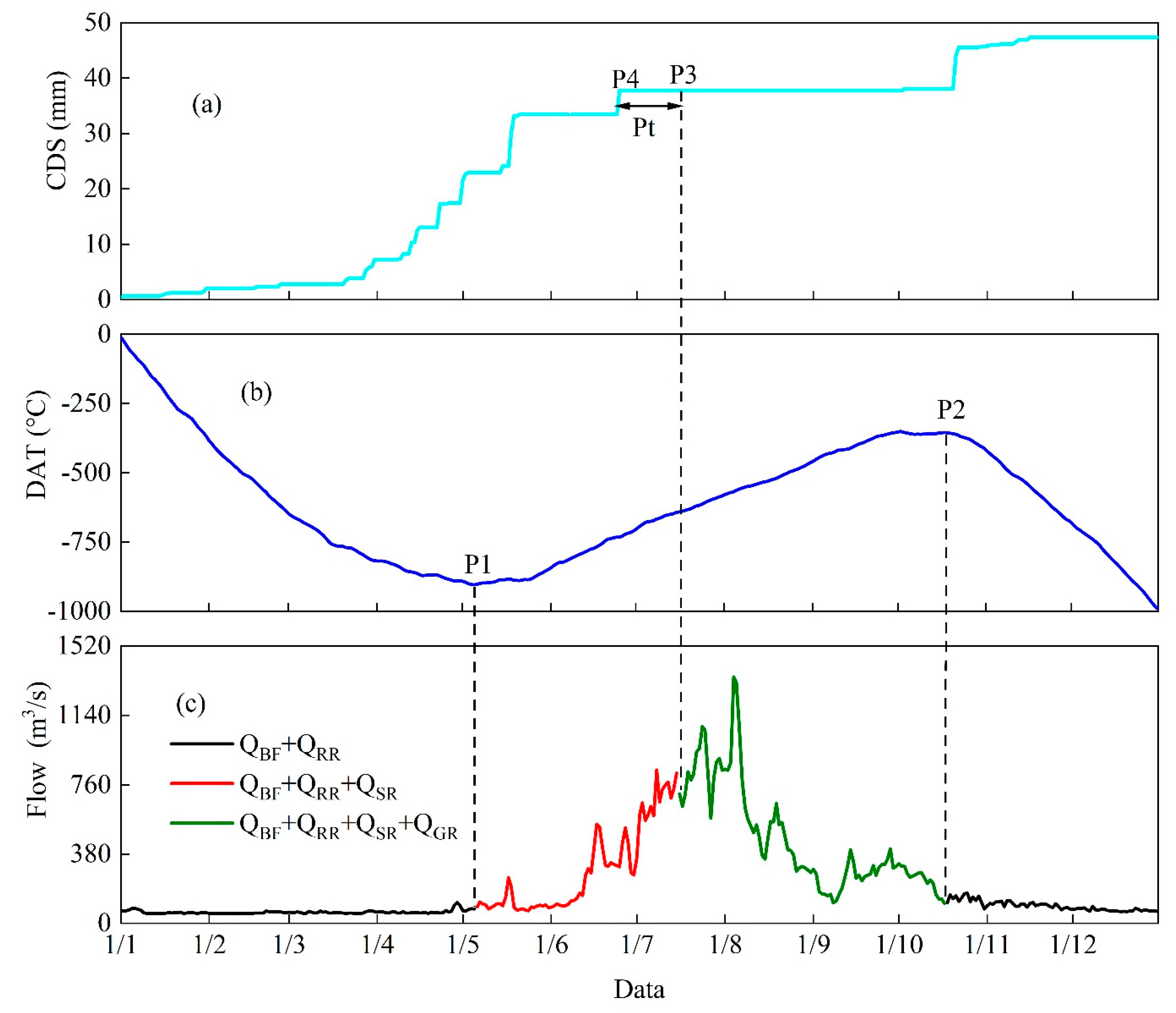
2.3.1. Hydrograph Partitioning Curves

Different parts of the hydrograph can be dominated by different hydrographs, which are expressed and simulated by the corresponding constitutive equations and parameters in the hydrograph. The hydrograph is divided into corresponding segments based on temperature and precipitation, called hydrograph partitioning curves (HPC) [38,39]. The HPC is a method for dividing the runoff hydrograph subsets of alpine watersheds based on the potential hydrological information. The method considers that rainfall runoff mainly occurs in the rainy season, while glaciers and snowpacks have different elevational distribution ranges. There is a specific seasonal difference in the occurrence period of runoff. The minimum distribution elevation of snowpack is often lower than that of glaciers, and snowmelt runoff generally starts at a lower elevation band than glacier melt runoff. Since the temperature in the alpine basin significantly decreases with the elevation increase, there is a period in which the temperature at the lowest altitude where the snowpack is located has exceeded the melting temperature threshold. However, the lowest altitude where the glaciers are located has not yet reached the temperature threshold. That is, snowmelt runoff can occur while glacier melt runoff cannot. In addition, neither meltwater runoff nor rainfall surface runoff occurs when the study period is not in the rainy season; the temperature at the lowest elevation of snowpack does not exceed the melting temperature threshold, and total runoff in this period consists entirely of baseflow [38,39].

The average daily precipitation and temperature of the Lhasa River Basin during the study period from 2010 to 2019 were calculated to extract the HPC. Assuming that the precipitation when the temperature is lower than 0 °C is snowfall, the cumulative curve of daily snowfall (CDS) was obtained by superimposing the precipitation when the temperature is less than 0 °C, and the daily precipitation is greater than 0 mm. Additionally, the daily accumulated temperature (DAT) curve was obtained from the accumulation of the average daily temperature of the entire basin. Figure 2 shows an example of the extraction of HPCs in 2011. This scenario considers that the total runoff is mainly composed of base flow before the accumulated temperature reaches the minimum point (P1) and after the maximum point (P2). The turning point (P4) on the CDS curve, followed by the longest non-snowy period, indicates the end of snow accumulation. A period after the P4 point indicated by the Pt value (assume four weeks [39]) was adopted to represent the persistence of snow accumulation after the last snowfall event [38,39]. The snowmelt process between the P1 and P3 points dominates the hydrological process. It was assumed that the snowpack had melted, and the glacier began to melt at the P3 point. There may be rainfall runoff on the date of occurrence of rainfall with no consideration given to the impact of rainfall. Based on the above logic, the flow hydrograph was divided into three stages, as shown in Figure 2c. According to the above steps, the division of flow hydrographs dominated by different water sources could be realized.

2.3.2. Spatial Processes in Hydrology Model

The SPHY model (v2.0, http://www.sphy.nl/, accessed on 24 December 2021) is a spatially distributed hydrology model applied cell-by-cell, where the cell value represents the average value of an attribute within a cell, which may be precipitation, air temperature, soil layer thickness, DEM, etc. The model is written in Python using the PCRaster dynamic modeling framework [15], based on QGIS software as a platform, including soil, glacier, evapotranspiration, snowpack, groundwater module, and confluence in six integrated modules, as well as an extension module. The model is mainly divided into the glacier-covered area and non-glacier-covered area. The soil structure of a non-glacier-covered area includes three layers: root zone layer, sub-root zone layer, and groundwater layer.

In the SPHY model, the calculation process of snowpack melting and glacier melting adopts the degree-day model based on an empirical relationship between melt rate and air temperature [15]. In the snowpack module of the SPHY model, processes such as the potential and actual ablation volume of snowpack, water-holding capacity of snowpack, refreezing of melting snowpack, and runoff produced by snowpack melting are considered. Since the melting rates of debris-covered and debris-free glaciers vary for glacier ablation, these two glaciers need different degree-day factors to separately simulate their ablation processes [15]. The SPHY model divides the study area into many identical cells. Due to the uneven spatial distribution of hydrometeorological elements in the watershed and the characteristics of the underlying surface, each cell simulates hydrological processes such as precipitation, evaporation, infiltration, glacier, and snowpack melting according to the input elements and obtains the runoff of each cell. When a cell encounters the runoff of the adjacent upstream grid, it will conduct a confluence calculation to the adjacent downstream grid through the surface confluence path. The recession coefficient represents the lag characteristics of the catchment in the basin. When the total runoff of several cells is calculated through the above process, the total runoff of the outlet section of the entire watershed can be obtained. The SPHY model divides the total runoff at the outlet into four parts: rainfall runoff, snowmelt runoff, glacier melt runoff, and baseflow when calculating confluence [15]. The calculation formula for total runoff is as follows:

$$Q_{TR}=Q_{BF}+Q_{RR}+Q_{SR}+Q_{GR}$$

(1)

where, $Q_{TR}$, $Q_{BF}$, $Q_{RR}$, $Q_{SR}$, and $Q_{GR}$ are the total runoff, baseflow, rainfall runoff, snowmelt runoff, and glacier melt runoff, respectively.

2.3.3. Calibration of the SPHY Model

Considering that the actual measured daily runoff data of TANGJIA from 2009–2019 were collected in this study, and the relative geographical location of the two stations was that TANGJIA station was located upstream, the actual measured flow data of the TANGJIA station from 2010–2019 (2009 was the warming-up period) were used to calibrate the SPHY model in this study. The data (2009–2019) from the LHASA station were mainly used to verify the simulation results.

The HPC division method was used to divide the measured daily runoff data of the TANGJIA hydrological station from 2010–2019 into combinations of different runoff components. Then, the parameter calibration of the SPHY model was carried out in 4 approaches based on the results of the runoff division, as shown in

Table 2. Stepwise calibration of SPHY model parameters based on the HPC division method.

Step	Subsets of Hydrological Process	Objective Function	Parameters
1	$Q_{BF}+Q_{RR}$	$NSE$ $R^2$ $RMSE$	GwDepth, GwSat, deltaGw, alphaGw
2	$Q_{BF}+Q_{RR}+Q_{SR}$		DDFS, Tcrit, SnowSC
3	$Q_{BF}+Q_{RR}+Q_{SR}+Q_{GR}$		DDFG, DDFDG, Glacf
4	$Q_{TR}$		RootDepthFlat, SubDepthFlat, CapRiseMax, kx

. Steps 1 to 3 were used to calibrate the constitutive parameters of the corresponding hydrological process based on the flow process lines dominated by baseflow, snow melt, and glacier melt. Step 4 determined other parameters that could not be divided into steps 1–3. To evaluate the performance of the SPHY model for simulating daily runoff, the leading evaluation indicators adopted in this study were as follows: the Nash-Sutcliffe efficiency ($NSE$, Equation (2)), coefficient of determination ($R^2$, Equation (3)), and root mean square error ($RMSE$, Equation (4))

$$NSE=1-\frac{{{\displaystyle \sum }}_1^n{\left(Q_{obs,i}-Q_{sim,i}\right)}^2}{{{\displaystyle \sum }}_1^n{Q}_{obs,i}-\frac{1}{n}{\left({{\displaystyle \sum }}_1^n{Q}_{obs,i}\right)}^2}$$

(2)

$$R^2=\frac{{{\displaystyle \sum }}_1^n{\left[\left(Q_{obs,i}-\overline{Q_{obs,i}}\right)\left(Q_{sim,i}-\overline{Q_{sim,i}}\right)\right]}^2}{{{\displaystyle \sum }}_1^n{\left(Q_{obs,i}-\overline{Q_{obs,i}}\right)}^2{{\displaystyle \sum }}_1^n{\left(Q_{sim,i}-\overline{Q_{sim,i}}\right)}^2}$$

(3)

$$RMSE=\sqrt{\frac{1}{n}{{\displaystyle \sum }}_1^n{\left(Q_{obs,i}-Q_{sim,i}\right)}^2}$$

(4)

where $n$ is the time-step of daily observed runoff and daily simulated runoff; $Q_{obs,i}$ (m³/s) and $Q_{sim,i}$ (m³/s) are the daily observed runoff and daily simulated runoff on day $i$, respectively; $\overline{Q_{obs,i}}$ (m³/s) and $\overline{Q_{sim,i}}$ (m³/s) are the daily observed runoff and daily simulated runoff, respectively.

The parameter estimation (PEST) [45,46,47] hydrological parameter estimation model, which is model-independent parameter estimation software that undertakes the task of uncertainty analysis, is adopted to optimize the parameters of the SPHY model. The PEST was published in 1999 and experienced rapid development. The software has been used in many fields, such as mechanical manufacturing, aeronautical design, and hydrological modeling. The principle of PEST parameter adjustment is to change each parameter, determine their respective sensitivity to the model, and establish the process of parameter adjustment direction according to the difference in sensitivity. After continuous parameter adjustment, the simulated output of the model gets closer to the measured value used for correction. Finally, the simulation effect is optimized to determine the model’s parameters.

2.3.4. Statistical Downscaling Model

The SDSM couples weather generators and multiple linear regression to downscale by establishing relationships between global predictors and forecast quantities, such as temperature and precipitation [48]. According to the established model, selecting a specific GCM can predict and analyze the changes in meteorological elements under different climate scenarios. In the downscaling process of the SDSM, the temperature simulation is regarded as an unconditional process, and the precipitation simulation is a conditional process.

When simulating precipitation, the SDSM simulates the probability of precipitation on a specific day. The amount of precipitation on rainy days can be calculated as (5):

$$W_i={\alpha }_0+{{\displaystyle \sum }}_{j=1}^n{\alpha }_j{x}_j+{\alpha }_{i-1}{W}_{i-1}$$

(5)

where, $W_i$ and $W_{i-1}$ are the probability of precipitation on day $i$, $i-1$, respectively; $x_j$ is the j global predictor; ${\alpha }_0$, ${\alpha }_j$ and ${\alpha }_{i-1}$ are regression coefficients.

A random number r determines precipitation occurrence ($0\le r\le 1$), conforming to a normal distribution. If $r$ < $W_i$, it is considered that there will be a precipitation event on day i. After determining the occurrence of a precipitation event on a specific day, the multiple exponential regression function is used to simulate the precipitation on day $i$.

$$R_i=exp\left({\beta }_0+{{\displaystyle \sum }}_{j=1}^n{\beta }_j{x}_j+{\epsilon }_i\right)$$

(6)

where, $R_i$ is the precipitation on day $i$; $x_j$ is the j global predictor; ${\beta }_0$ and ${\beta }_j$ are regression coefficients. ${\epsilon }_i$ is the random error term of a normal distribution.

There is a direct linear relationship between regional forecasts and selected predictors for unconditional simulation processes such as temperature.

$$T_i={\beta }_0+{{\displaystyle \sum }}_{j=1}^n{\beta }_j{x}_j+{\epsilon }_i$$

(7)

where, $T_i$ is the temperature on day $i$; $x_j$ is the j global predictor; ${\beta }_0$ and ${\beta }_j$ are regression coefficients. ${\epsilon }_i$ is the random error term of a normal distribution.

This study selected the measured daily precipitation; and maximum, average, and minimum temperature of meteorological stations from 2009 to 2017 in the Lhasa River Basin as predictands. Combined with many predictors of NCEP data (2009–2017), the statistical relationship between each predictor and the predictands was established. The SDSM model was established by selecting the optimal predictors according to the performance of the statistical relationship. According to the optimal predictors in the NCEP dataset, the predictors in the SSP1-2.6 and SSP2-4.5 scenario data (2020–2100) were selected. These predictors were imported into the constructed SDSM model to obtain the meteorological stations’ future daily precipitation and maximum, average, and minimum temperature in the Lhasa River Basin.

3. Results

3.1. Results of the HPC Division Method

The measured runoff at TANGJIA hydrological station from 2010 to 2019 is divided by composition by the HPC method. The results are shown in Figure 3. Figure 3 shows that the base flow is mainly concentrated in the preceding stage of each year. Combined with the average precipitation in the Lhasa River Basin, the precipitation during this period is relatively small. Snowmelt runoff occurs in the warming stage from spring to early summer every year. The runoff is mainly supplied by snowmelt during this stage, with rising temperatures and no significant increase in precipitation. Notably, the end time of this stage varies in different years, especially the ratio of end-to-peak runoff to peak runoff varies greatly. In dry 2011, the flow at the end of the snowmelt-dominant period accounted for two-thirds of the peak flow. On the contrary, 2019 was a wet year, and the flow at the end accounted for only a tiny percentage of the peak flow. The peak value of the glacier melt runoff has a corresponding positive relationship with the peak value of precipitation, mainly concentrated in the summer with abundant precipitation and high temperature.

In order to verify the reliability of the classification results of the HPC, further comparisons were made with the average snowpack cover area of the Lhasa River Basin observed by remote sensing, as shown in Figure 3b. As shown, the proportion of snowpack cover area and runoff are inversely related. The snowpack cover area is prominent in the low flow period and vice versa. Further analysis shows that the dominant snowmelt period of each year is the stage in which the snowpack cover area of the Lhasa River Basin gradually decreases, which further indicates the rationality of the division results of the hydrograph.

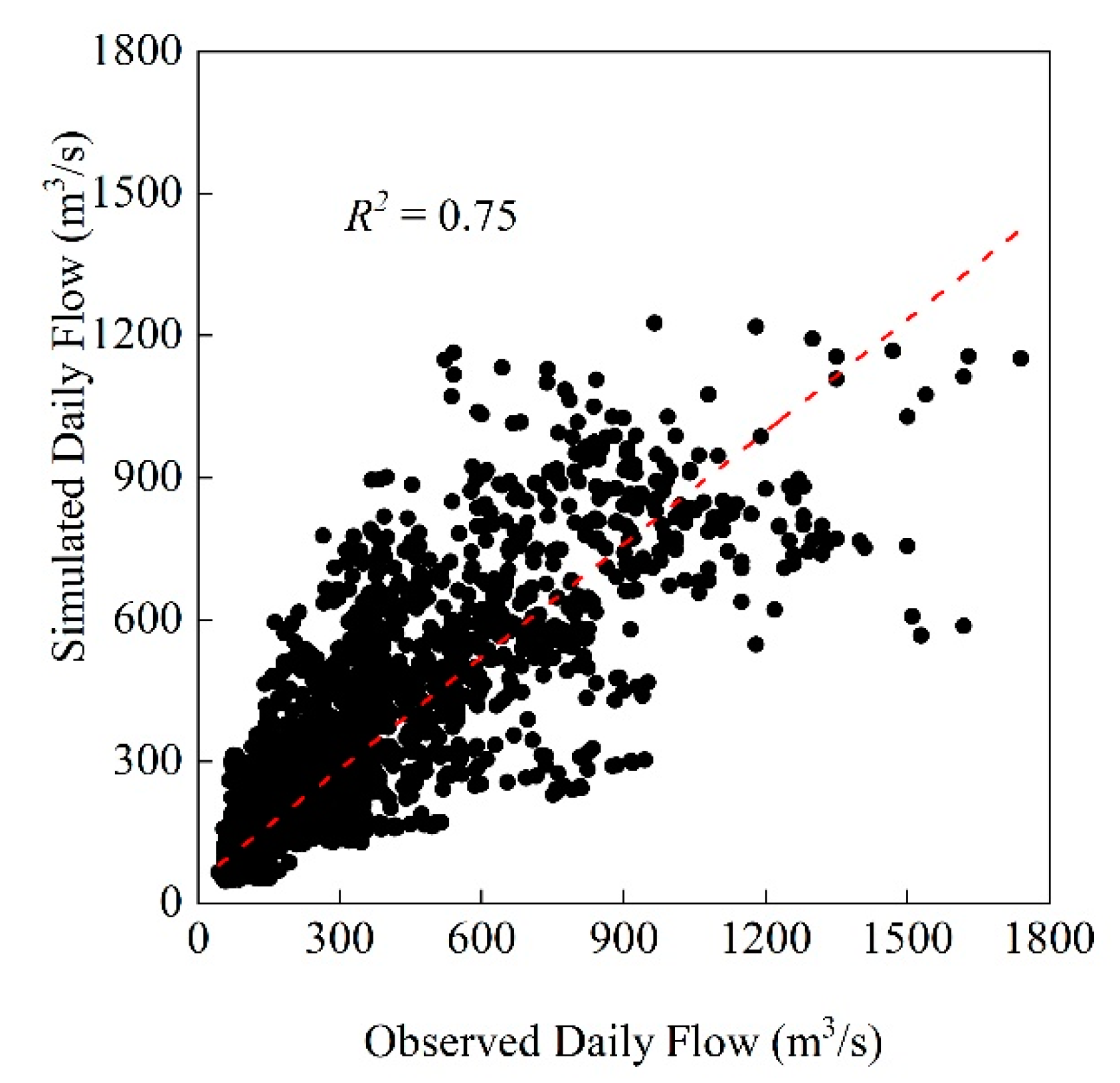
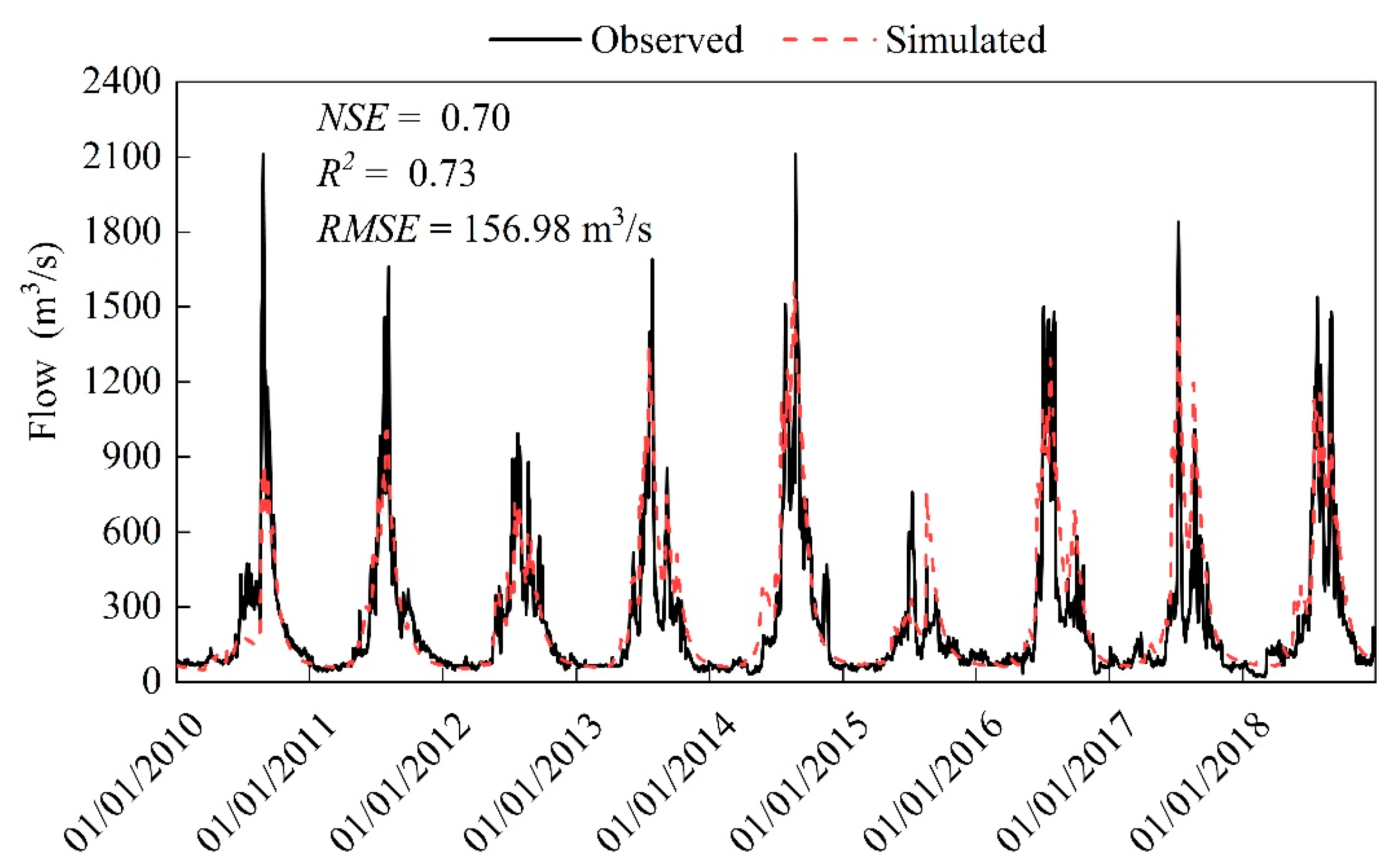
3.2. Performance of the SPHY Model

The parameters of the SPHY model were optimized using the PEST software according to the calibrating steps in Table 2, and the optimal parameter values calculated are shown in

Table 3. Calibrated SPHY model parameter values used for the simulation.

NO.	Name of the Parameter	Description (Unit)	Fitted Value
1	GwDepth	Groundwater layer thickness (mm)	3000.00
2	GwSat	Saturated groundwater content (mm)	2000.00
3	deltaGw	Delay time (d)	0.01
4	alphaGw	Baseflow recession coefficient (-)	0.003
5	DDFS	Snow degree-day factor (mm degree−1 day−1)	0.85
6	Tcrit	Temperature threshold for precipitation to rainfall as snow (°C)	0.00
7	SnowSC	Water storage capacity (mm mm−1)	0.18
8	DDFG	Glacier clean ice degree-day factor (mm degree−1 day−1)	19.89
9	DDFDG	Glacier debris degree-day factor (mm degree−1 day−1)	20.00
10	Glacf	Glacier melt runoff factor (-)	0.22
11	RootDepthFlat	Rootzone depth (mm)	146.41
12	SubDepthFlat	Sublayer thickness (mm)	501.18
13	CapRiseMax	The maximum amount of water from the subzone to the rootzone	0.85
14	kx	Recession coefficient of routing	0.95

.

At the TANGJIA hydrologic station, the R², NSE, and RMSE between the measured flow and simulated flow from the SPHY model were 0.75, 0.75, and 126.87 m³/s, respectively. According to the criteria prescribed by [49,50], all these indices are in the ‘good’ category, showing that the simulation results of the SPHY model are acceptable. The time series plots and scatter plots between observed and simulated flow shown in Figure 4 and Figure 5 indicate that simulated flow at the TANGJIA station significantly captures low flow values as the observed values. Additionally, the figure shows that the SPHY model has a poor simulation effect on peak flow, especially in 2015. The peak occurrence time was deviated, which may be caused by the error in rainfall data.

In order to further validate the reliability of the results of the HPC stepwise calibrating the SPHY model, the flow value of the LHASA hydrological station in the basin was used to analyze the simulation results. As shown in Figure 6, the NSE, R², and RMSE were 0.70, 0.73, and 156.98 m³/s during the simulation period (2010–2018), respectively. Although the evaluation metrics of the LHASA station were slightly lower than that of the TANGJIA station, the peak flow and baseflow process were simulated well by the SPHY model. This, the SPHY model is feasible to simulate runoff in the Lhasa River Basin.

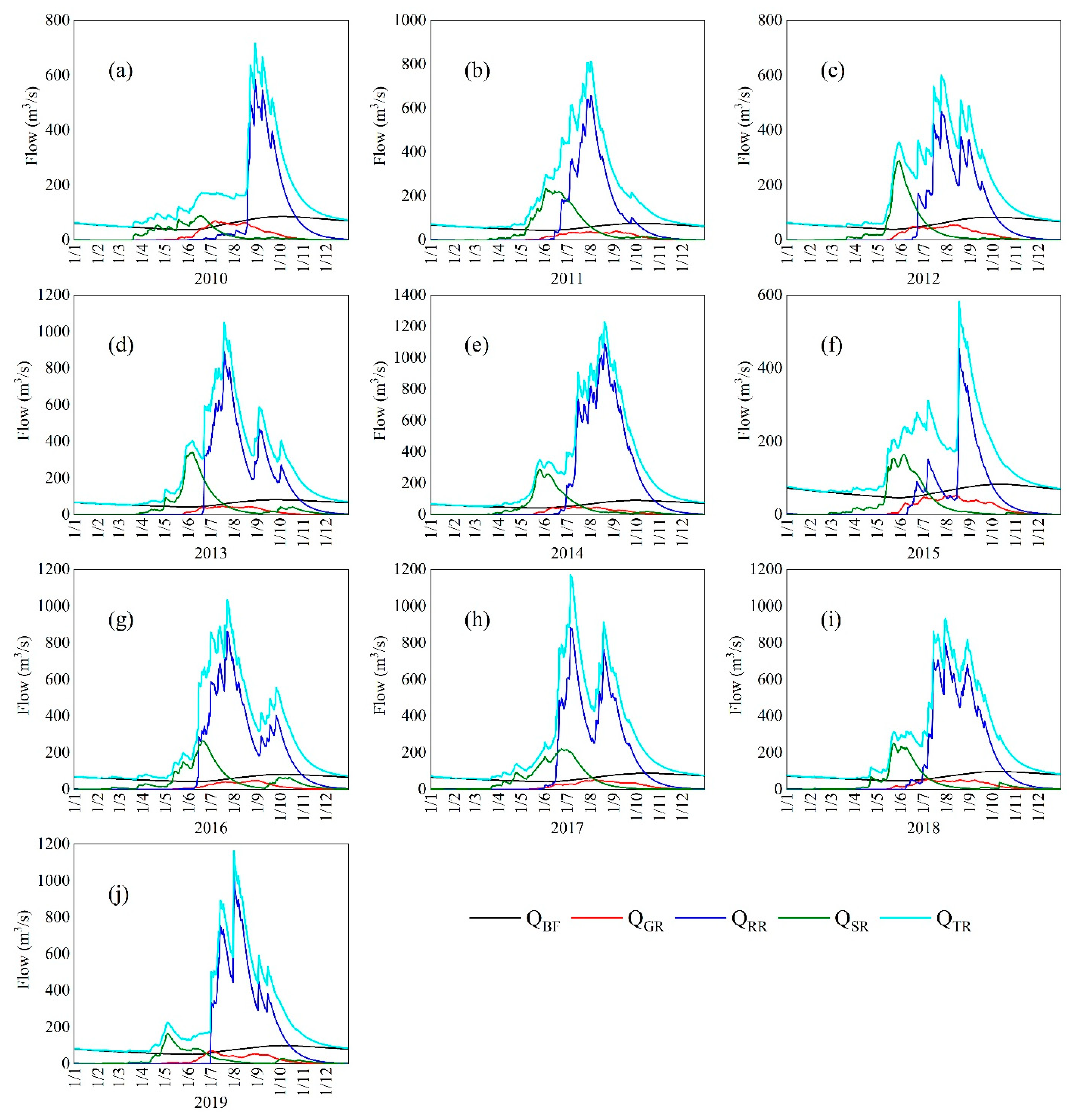
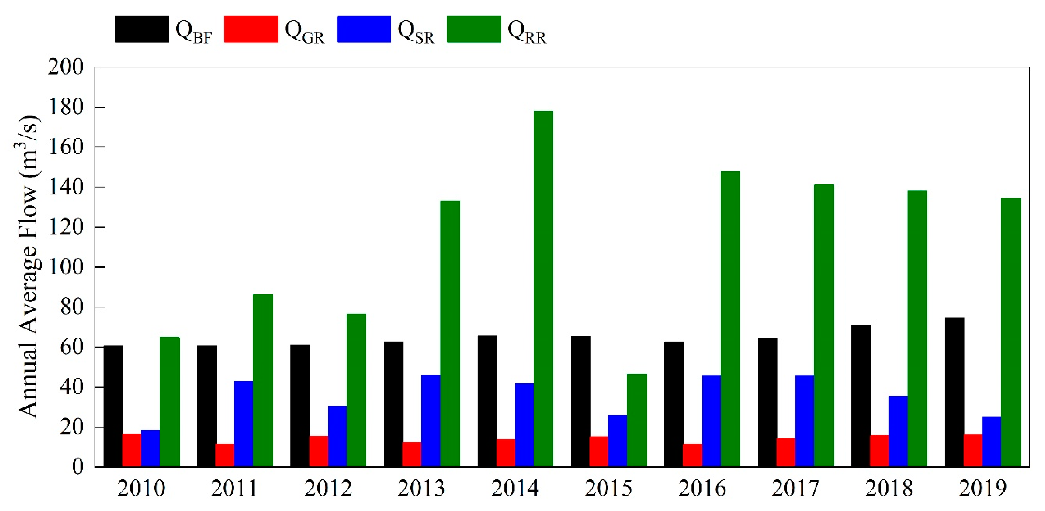
3.3. Assessments of Runoff Components

Figure 7 shows the variation in different runoff components computed by the SPHY model, including rainfall-runoff, snowmelt runoff, glacier melt runoff, and baseflow in the Lhasa River Basin in the year. As shown in Figure 7, baseflow is very stable without significant variation for each year. The baseflow value is slightly lower in June and July than in other months. Snowmelt runoff starts around the same time in different years, generally starting in April and continuing through October. Glacier melt runoff generates later than snowmelt runoff, generally starting in May, peaking in July, August and September, and ending in October. The duration of glacier melt runoff is shorter than the other three components. Although May to September is the rainy season in the Lhasa River Basin, Figure 7 shows that rainfall runoff is mainly concentrated from June to September annually. This phenomenon may be because rainfall-runoff produces a certain degree of hysteresis effect.

Figure 8 shows the interannual variations of each component from 2010 to 2019. The diagram shows that the annual mean flow values of baseflow and glacier melt runoff are very stable between different years, whereas the annual mean flow values of rainfall runoff and snowmelt runoff show significant variations. Especially for rainfall runoff, annual mean flow values range from around 46.32~177.96 m³/s. The multi-year averages of total flow, baseflow, glacier melt runoff, snowmelt runoff, and rainfall runoff from 2010 to 2019 are 229.33, 64.80, 14.24, 35.72, and 114.57 m³/s, respectively. Figure 9 shows the mean annual contributions of each component to the total runoff from 2010 to 2019. Among all components, rainfall-runoff contributes 49.98% and has the most considerable contribution to total runoff, followed by baseflow, snowmelt runoff, and glacier melts runoff, contributing 28.26%, 15.57%, and 6.19%, respectively.

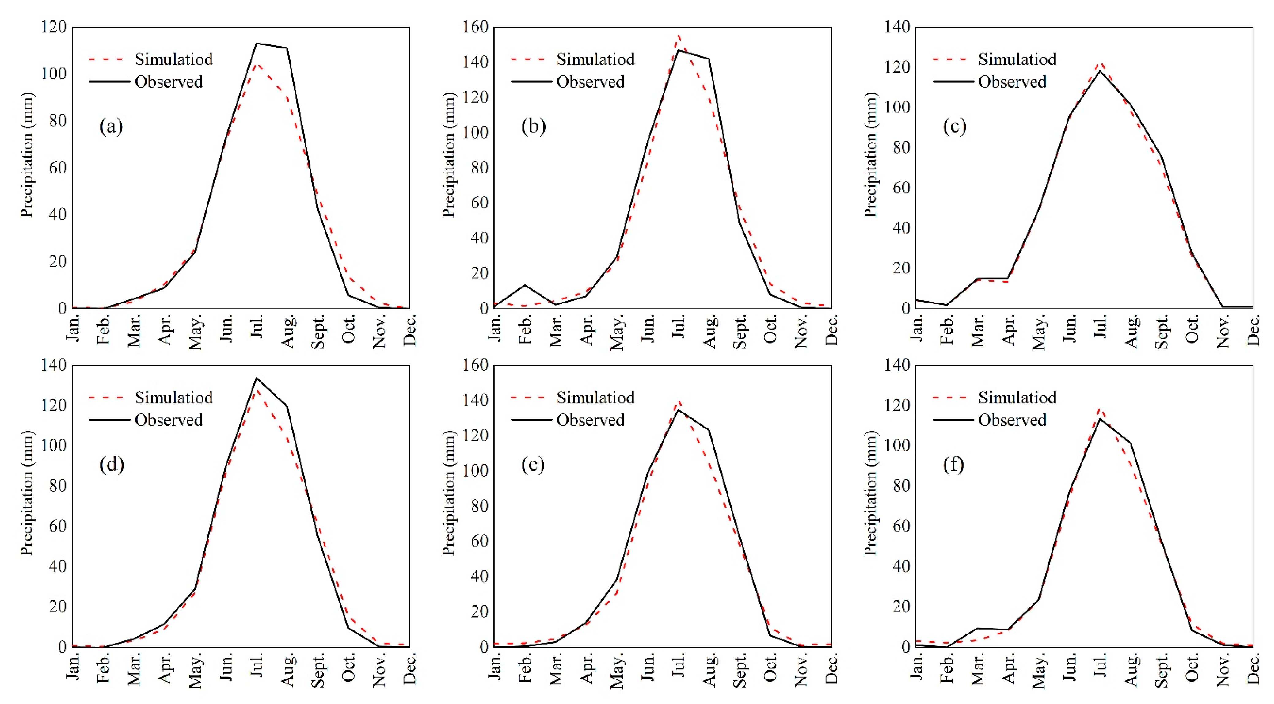
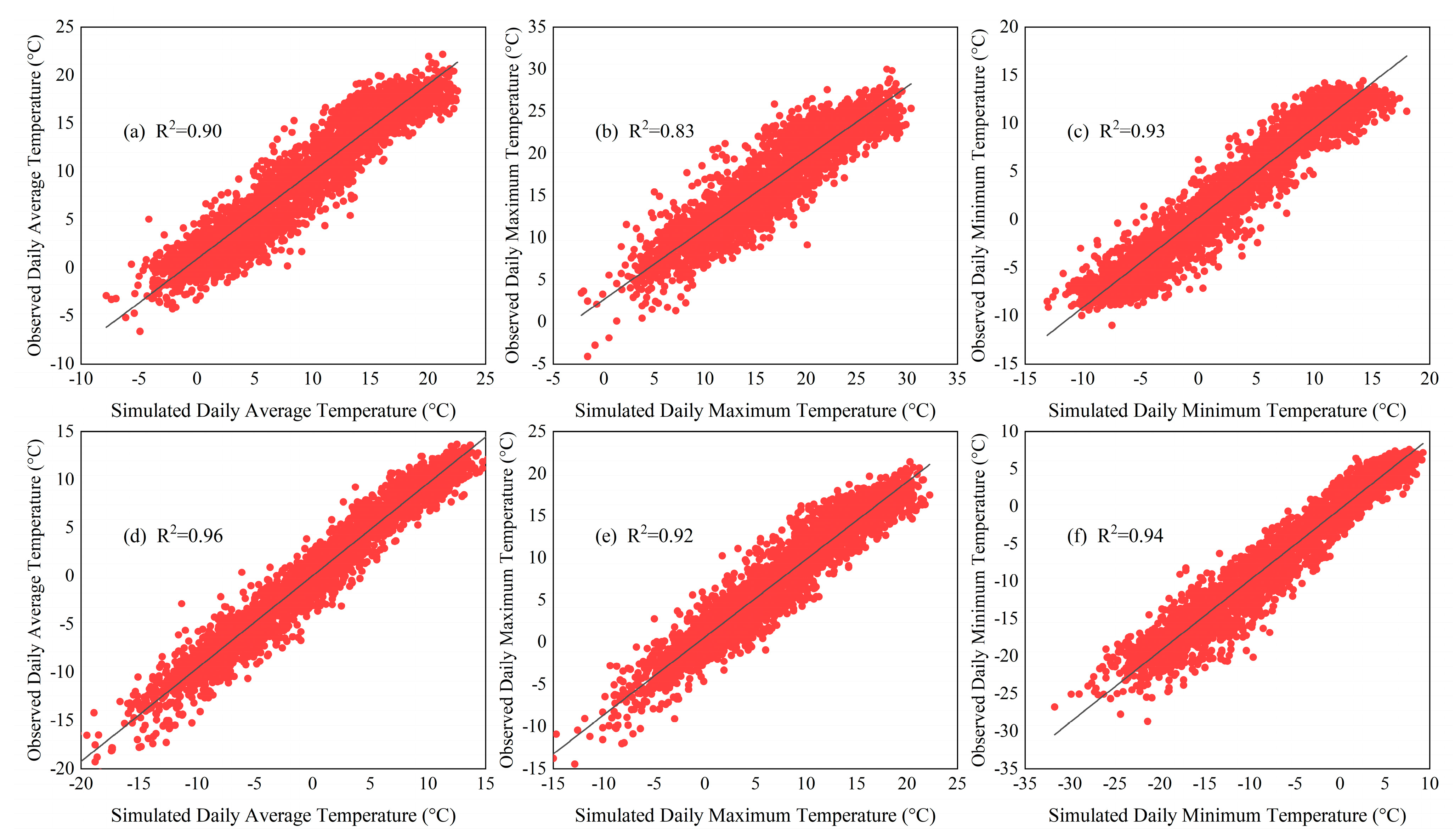
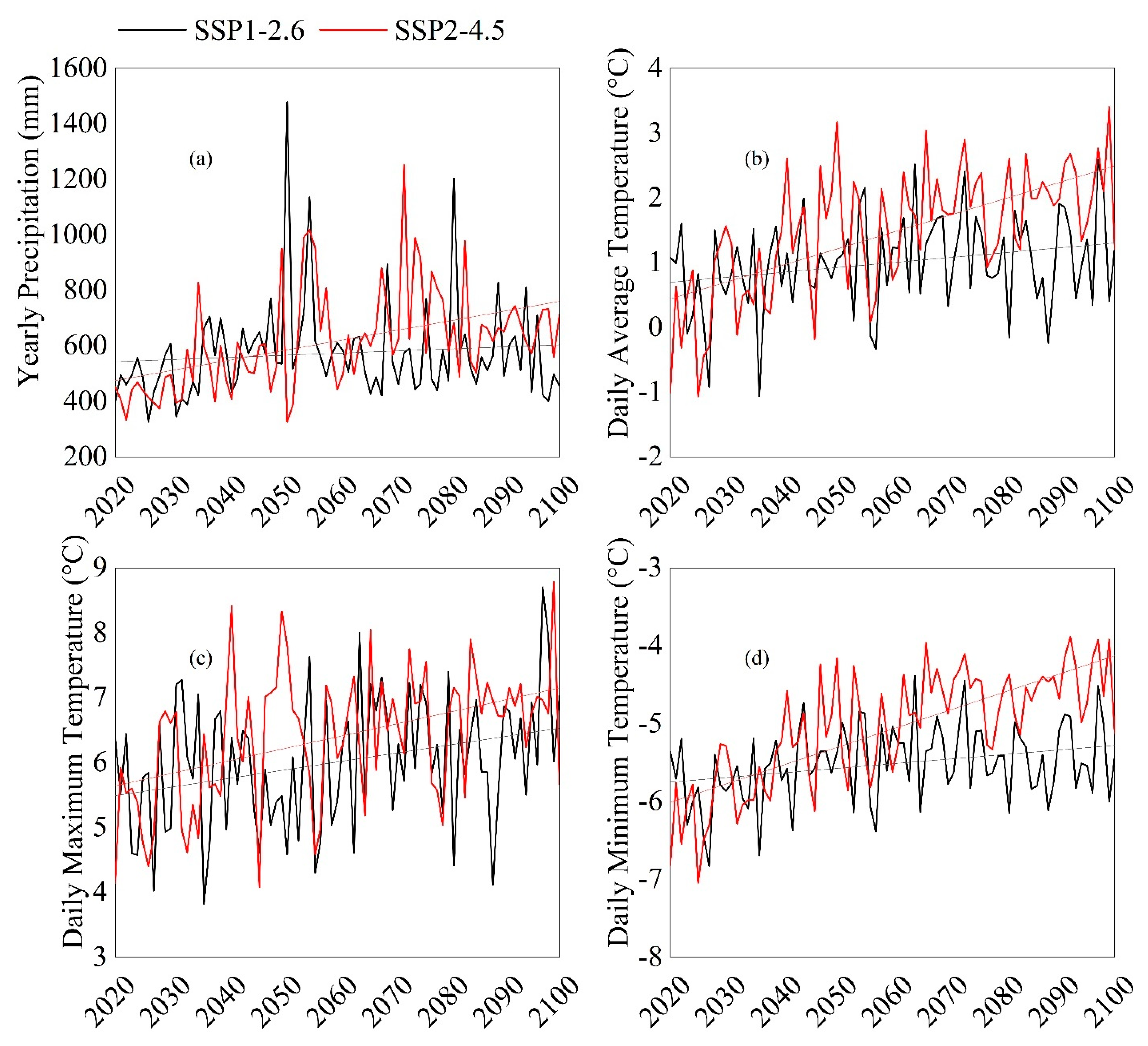
3.4. Results of the SDSM

The selected NCEP predictor and SDSM model were used to simulate the precipitation of six meteorological stations and the temperature of two meteorological stations in the Lhasa River Basin. Figure 10 compares the measured and simulated monthly mean precipitation. It can be seen from Figure 10 that the measured values of monthly average precipitation from the meteorological stations in the Lhasa River Basin fit well with the simulated values of the SDSM from 2009 to 2017. It shows that the SDSM has good applicability in the Lhasa River Basin, with more reliability in the downscaling precipitation simulation. The scatter plots between measured and simulated daily average, maximum, and minimum temperatures of LASHA and NAGQU stations are shown in Figure 11. Except for the R² value calculated from the measured and simulated daily maximum temperature at the LHASA station of less than 0.9, the rest of the R² s are more significant than 0.9, which suggests that SDSM is feasible to predict future climate changes in the Lhasa River Basin.

Subsequently, the future CanESM5 climate model data (2020–2100) was imported into the calibrated SDSM to generate the daily precipitation; and maximum, minimum, and average temperature of the meteorological stations under the two shared socioeconomic pathways (SSP1-2.6, SSP2-4.5). The daily precipitation data in the Lhasa River Basin is calculated by the Thiessen polygon method. The daily average, maximum and minimum temperature values are obtained by interpolation with an elevation effect.

The line graphs (Figure 12) show that computed yearly precipitation; and daily average, maximum and minimum temperature vary by year. The trend line added in Figure 12 shows that the meteorological data in the Lhasa River Basin fluctuates significantly, showing an increasing trend.

Table 4. Increasing rate of yearly precipitation; daily average, maximum, and minimum temperature.

Type of SSP	Increasing Rate of Annual Precipitation (mm/a)	Increasing Rate of Daily Average Temperature (°C/10a)	Increasing Rate of Daily Maximum Temperature (°C/10a)	Increasing Rate of Daily Minimum Temperature (°C/10a)
SSP1-2.6	0.76	0.08	0.13	0.06
SSP2-4.5	3.57	0.25	0.19	0.24

shows that the increasing rate of meteorological data varies greatly among different SSPs. Under SSP2-4.5 scenario, increasing the yearly precipitation rate, daily average maximum, and minimum temperature is faster, up to 3.57 mm/a, 0.25, 0.19, and 0.24 °C/10a, respectively. However, under the SSP1-2.6 scenario, the increasing rates are only 0.76 mm/a, 0.08, 0.13, and 0.06 °C/10a respectively.

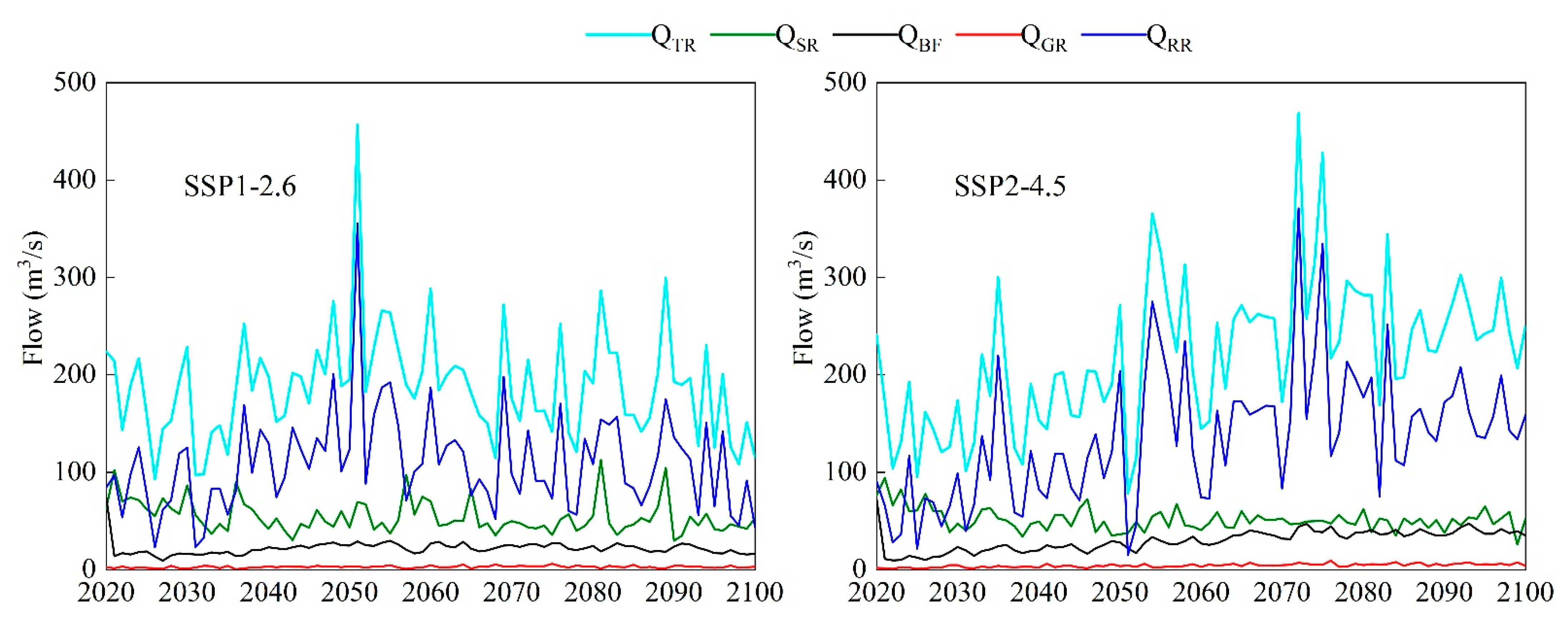
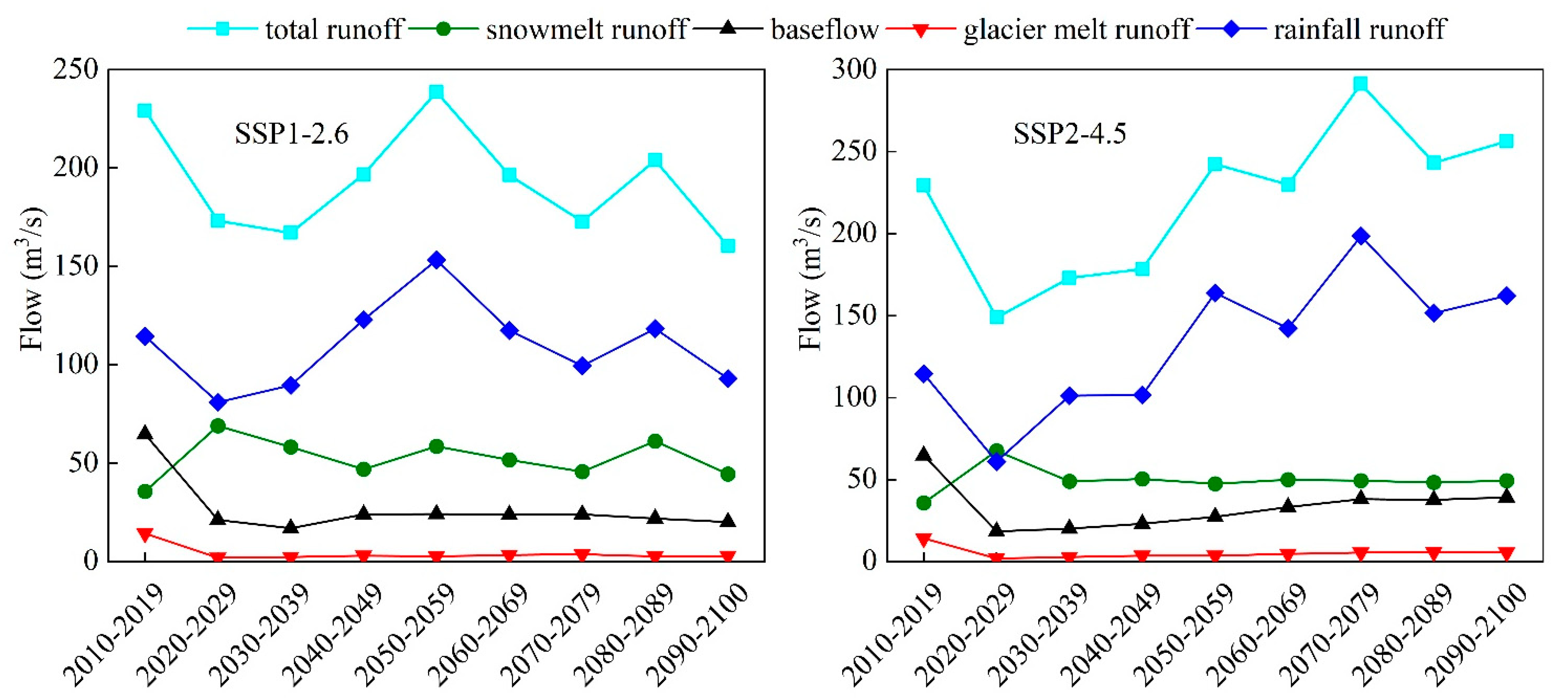
3.5. Runoff Response under Future Climate Scenarios

The daily precipitation; and average temperature, maximum temperature, and minimum temperature of each meteorological station generated by SDSM under the SSP1-2.6 and SSP2-4.5 scenarios were input into the SPHY model calibrated to obtain the future variation of the runoff and components of the Lhasa River.

The changing trend in annual runoff in the future is shown in Figure 13.

Table 5. Change rate of total runoff, snowmelt runoff, baseflow, glacier melt runoff, and rainfall runoff (m³/s/year).

	Total Runoff	Snowmelt Runoff	Baseflow	Glacier Melt Runoff	Rainfall-Runoff
SSP1-2.6	−0.31	−0.02	−0.27	−0.07	0.04
SSP2-4.5	1.13	−0.01	0.01	−0.03	1.16

shows that under the SSP1-2.6 scenario, the total runoff of the Lhasa River is a slowly decreasing trend with a rate of 0.31 m³/s per year, which is mainly attributed to the reduction of baseflow. Although rainfall runoff shows an upward trend, snowmelt runoff, and glacier melt runoff show a downward trend, all have little effect on the total runoff. Under the SSP2-4.5 scenario, the total runoff from the Lhasa River is a clear upward trend at a rate of 1.13 m³/s per year, which is mainly attributed to the increase in rainfall in the Lhasa River basin, resulting in an apparent increase in rainfall runoff at a rate of 1.16 m³/s per year. The remaining variations in baseflow, snowmelt runoff, and glacier melt runoff have little effect on the total runoff. In both scenarios, snowmelt runoff and glacier melt runoff are decreasing, which may be related to the reduction in snowfall and ablation of marginal glaciers due to future temperature increases in the Lhasa River Basin.

4. Discussion

As shown in Figure 2, the runoff that occurred from May to mid-July 2011 is mainly composed of baseflow, rainfall runoff, and snowmelt runoff. In Figure 7b, the simulation results of the SPHY model in the same period in 2011 show the runoff was mainly composed of these three components. From mid-July to mid-October 2011, the HPC division and SPHY simulations show that glacier melt runoff components are in the total runoff during this period. In addition to 2011, there are similar division results and corresponding simulation results in other years. These similarities suggest that our partitioning runoff processes using the HPC method are more reasonable. In Figure 7, the interval between the occurrence time of snowmelt runoff and glacier melt runoff is different in different years. For example, in 2013, the interval was approximately eight weeks, while in 2019, the interval was only about three weeks. These intervals differ from the Pt value (recommended four weeks [39]) we determined in the HPC method. Therefore, in future research, it is necessary to determine the Pt value more accurately according to the characteristics of the study area.

Based on the SRM model and MODIS data, the study has simulated that the contribution rate of snowmelt runoff to the total runoff in the Lhasa River Basin from 2002 to 2003 was 3% to 6% [9]. Many studies have analyzed the runoff components of the Yarlung Zangbo River Basin, where the Lhasa River is located. Using the variable infiltration capacity (VIC) model, Zhang et al. [51] determined the proportion of snowmelt runoff and glacier melt runoff in the Yarlung Zangbo River from 1961 to 1991 was 23.0% and 11.6%, respectively. Using the coupled routing and excess storage (CREST) model, Chen et al. [52] found that the proportions of snowmelt runoff and glacier melt runoff from 2003 to 2015 were 10.6% and 9.9%, respectively. Using the SRM model, Bookhagen et al. [53] found that the proportion of snowmelt runoff and glacier melt runoff from 2000 to 2007 was 34.4%. This study concludes that from 2010 to 2019, the proportion of snowmelt runoff and glacier melt runoff in the Lhasa River was 15.57% and 6.19%, respectively, and the total is 21.79%. Compared with these studies, we can see that the proportion of this study is small, but all of the studies indicate that snowmelt runoff and glacier melting runoff are essential components of the runoff of the Lhasa River and even the Yarlung Zangbo River. The difference may be due to the different study periods and the uncertainty of hydrological models in the runoff simulation. This study adopts a physical-based hydrograph division method and corresponding stepwise calibration method. It obtains more reasonable model parameters, which are more consistent with the measured runoff process. From this perspective, the findings on runoff components from this study’s application of the HPC method are closer to reality.

According to previous research [54], the linear warming trends of the Qinghai-Tibet Plateau under different scenarios from 2015 to 2100 were pretty different. Under the SSP1-2.6 and SSP2-4.5 scenarios, the warming rate is 0.10 and 0.29 °C per decade, respectively, close to the temperature-increasing rate in the study. Under the SSP2-4.5 scenario, the temperature-increasing rate of the Qinghai-Tibet Plateau is higher than the current global warming rate of nearly 0.2 °C per decade, as pointed out in the IPCC Special Report on Global Warming of 1.5 °C [55]. The difference between the two shows that Qinghai-Tibet Plateau is more sensitive to global warming.

Figure 14 depicts the average flow of various runoff components per decade. It can be seen from the figure that the snowmelt runoff has the same trend in both scenarios. Snowmelt runoff increases from the 2010–2019 period to the 2020–2029 period. After the 2020–2029 period, the snowmelt runoff shows a decreasing trend. This change may be because the snowmelt rate increases as the temperature rises, causing the snowmelt runoff to rise in the early stage. However, as the snow continues to melt, the snow cover area decreases, which will offset the effect of the increase in the snowmelt rate and change the snowmelt runoff into a downward trend. The changes in glacier runoff are directly affected by the increase in temperature. Global warming has led to a sharp decrease in the area of glaciers on the Qinghai-Tibet Plateau from 2010 to 2019, and abundant runoff will be generated by glacial ablation. Consequently, there is less glacier melt runoff due to a lack of enough glaciers. Rainfall runoff is less affected by temperature changes. The total runoff is mainly affected by rainfall runoff, so the changing trend is similar to rainfall runoff. Baseflow is mainly recharged by rainfall and glacial meltwater [15]. From the 2010–2019 period to the 2020–2029 period, the decrease in rainfall and glacier meltwater resulted in a significant reduction in baseflow. The SSP2-4.5 scenario shows that the baseflow has an apparent increasing trend, which may be due to the more noticeable increase in rainfall in this scenario than in the SSP1-2.6 scenario.

Notably, according to the simulation results, the contribution rate of runoff components in the Lhasa River has significantly changed compared with that in the last decade of this century. Under the SSP1-2.6 scenario, rainfall runoff is still the largest, accounting for 57.99%, followed by snowmelt runoff, base flow, and glacier melt runoff, accounting for 27.72, 12.49, and 1.78%, respectively. The proportion of snowmelt runoff increased significantly, which may be due to the apparent reduction in total runoff and base flow. Under the SSP2-4.5 scenario, the proportion of rainfall runoff reached 63.31%, which was significantly more prominent. The apparent increase in rainfall may cause the phenomenon. The second is snowmelt runoff, base flow, and glacier melt runoff, accounting for 19.24, 15.27, and 2.17%, respectively.

According to the simulation results, snowmelt runoff and glacier melt runoff account for a large proportion of Lhasa River’s total runoff. As the climate warms, melting snow and glaciers will accelerate and significantly impact the Lhasa River’s water resources. Firstly, more precipitation and higher temperatures in summer lead to more melting water from glaciers and snow, making the summer flood disaster more serious. Second, changes in snowmelt runoff and glacier melt runoff lead to a more uneven distribution of Lhasa River water resources during the year.

Two reservoirs have been built in the Lhasa River basin, among which Zhikong Reservoir has only the daily regulation capacity and little influence on the simulation results, so it is not considered in this study. Although Pangduo Reservoir has the capacity for annual regulation, the measured data of Pangduo hydrology station is taken as the input data of the SPHY model to eliminate the reservoir’s influence. In the future runoff simulation, the existing and to-be-built reservoirs on the Lhasa River will have an impact. This study does not consider the impact of reservoirs under future scenarios, which is an obvious shortcoming. Therefore, hydraulic structures will be crucial in future runoff simulations of the Lhasa River. Additionally, a GCM is adopted in this study, which will cause certain uncertainties. Multiple GCMs can be integrated into future studies to reduce future climate uncertainty.

5. Conclusions

This study built the SPHY model in the Lhasa River Basin and gradually optimized the model’s parameters using the outcomes of the HPC division method. The SDSM model and two scenarios from the CanESM5 dataset, SSP1-2.6 and SSP2-4.5, predicted precipitation and temperature in the Lhasa River Basin for 2020–2100. Combined with the predicted results, this study analyzed the future changes in Lhasa River runoff and its components, and the following conclusions were obtained.

(1) The R², NSE, and RMSE of the simulated and measured flows of the SPHY model at TANGJIA hydrological station are 0.75, 0.75, and 126.87 m³/s, respectively, and 0.70, 0.73, and 156.98 m³/s at the LHASA hydrological station, respectively, indicating that the simulation results of the SPHY model in the Lhasa River Basin are acceptable.

(2) The total runoff of the Lhasa River is divided into rainfall runoff, baseflow, snowmelt runoff, and glacier melt runoff based on the simulation results of the SPHY model. The multi-year average values of these components from 2010 to 2019 are 114.57, 64.80, 35.72, and 14.24 m³/s with the proportions of 49.98, 28.26, 15.57, and 6.19%, respectively. These results indicate that rainfall is the most important water recharge of the Lhasa River.

(3) In both scenarios of the CanESM5 dataset, the temperature and precipitation in the future (2020–2100) in the Lhasa River Basin show an increasing trend. The increase is more pronounced in the SSP2-4.5 scenario.

(4) Snowmelt runoff and glacier melt runoff show a decreasing trend under both future scenarios because of the temperature increase in the Lhasa River Basin. Under the SSP1-2.6 scenario, the Lhasa River’s total runoff will decrease at a rate of 0.31 m³/s per year due to the decrease in baseflow. Under the SSP2-4.5 scenario, the total runoff of the Lhasa River will increase at a rate of 1.13 m³/s per year, mainly attributed to the increase in rainfall runoff caused by increased rainfall.

References

1. Qiu, L.; Peng, D.; Hu, L.; Zhang, M. Simulation of snowmelt runoff in the LHASA river basin by MODIS and SRM. J. Beijing Normal Univ. Nat. Sci. 2013, 49, 152–156. [Google Scholar]
2. Hebert, R.; Lovejoy, S. Regional Climate Sensitivity- and Historical-Based Projections to 2100. Geophys. Res. Lett. 2018, 45, 4248–4254. [Google Scholar] [CrossRef]
3. Tian, F.; Xu, R.; Nan, Y.; Li, K.; He, Z. Quantification of runoff components in the Yarlung Tsangpo River using a distributed hydrological model. Adv. Water Sci. 2020, 31, 324–336. [Google Scholar]
4. Gao, Z.; Wang, X.; Yin, G. Isotopic effect of runoff in the Yarlung Zangbo River. Chin. J. Geochem. 2012, 31, 309–314. [Google Scholar] [CrossRef]
5. Liu, J.T.; Gao, Z.J.; Wang, M.; Li, Y.Z.; Yu, C.; Shi, M.J.; Zhang, H.Y.; Ma, Y.Y. Stable isotope characteristics of different water bodies in the Lhasa River Basin. Environ. Earth Sci. 2019, 78, 11. [Google Scholar] [CrossRef]
6. Yu, T.-T.; Gan, Y.-Q.; Zhou, A.-G.; Liu, C.-F.; Liu, Y.-D.; Li, X.-Q.; Cai, H.-S. Characteristics of Oxygen and Hydrogen Isotope Distribution of Surface Runoff in the Lhasa River Basin. Earth Sci. 2010, 35, 873–878. [Google Scholar] [CrossRef]
7. Beven, K.; Freer, J. Equifinality, data assimilation, and uncertainty estimation in mechanistic modelling of complex environmental systems using the GLUE methodology. J. Hydrol. 2001, 249, 11–29. [Google Scholar] [CrossRef]
8. Prasch, M.; Weber, M.; Mauser, W. Distributed modelling of snow- and ice-melt in the Lhasa River basin from 1971 to 2080. In Proceedings of the 25th General Assembly of the International Union of Geodesy and Geophysics, Melbourne, Australia, 28 June–7 July 2011. [Google Scholar]
9. Qiu, L.H.; You, J.J.; Qiao, F.; Peng, D.Z. Simulation of snowmelt runoff in ungauged basins based on MODIS: A case study in the Lhasa River basin. Stoch. Environ. Res. Risk Assess. 2014, 28, 1577–1585. [Google Scholar] [CrossRef]
10. Zhang, G.Q.; Xie, H.J.; Yao, T.D.; Li, H.Y.; Duan, S.Q. Quantitative water resources assessment of Qinghai Lake basin using Snowmelt Runoff Model (SRM). J. Hydrol. 2014, 519, 976–987. [Google Scholar] [CrossRef]
11. Choi, J.R.; Chung, I.M.; Jeung, S.J.; Choo, K.S.; Oh, C.H.; Kim, B.S. Development and Verification of the Available Number of Water Intake Days in Ungauged Local Water Source Using the SWAT Model and Flow Recession Curves. Water 2021, 13, 1511. [Google Scholar] [CrossRef]
12. Kumar, M.; Denis, D.M.; Kundu, A.; Joshi, N.; Suryavanshi, S. Understanding land use/land cover and climate change impacts on hydrological components of Usri watershed, India. Appl. Water Sci. 2022, 12, 39. [Google Scholar] [CrossRef]
13. Alipour, M.; Hosseini, M. Simulation of surface runoff in Karaj dam basin, Iran. Appl. Water Sci. 2018, 8, 147. [Google Scholar] [CrossRef]
14. Pandey, B.K.; Gosain, A.K.; Paul, G.; Khare, D. Climate change impact assessment on hydrology of a small watershed using semi-distributed model. Appl. Water Sci. 2017, 7, 2029–2041. [Google Scholar] [CrossRef] [Green Version]
15. Terink, W.; Lutz, A.F.; Simons, G.W.H.; Immerzeel, W.W.; Droogers, P. SPHY v2.0: Spatial Processes in HY drology. Geosci. Model Dev. 2015, 8, 2009–2034. [Google Scholar] [CrossRef] [Green Version]
16. Lutz, A.F.; Immerzeel, W.W.; Shrestha, A.B.; Bierkens, M.F.P. Consistent increase in High Asia’s runoff due to increasing glacier melt and precipitation. Nat. Clim. Change 2014, 4, 587–592. [Google Scholar] [CrossRef] [Green Version]
17. Wu, J.K.; Li, H.Y.; Zhou, J.X.; Tai, S.Y.; Wang, X.L. Variation of Runoff and Runoff Components of the Upper Shule River in the Northeastern Qinghai-Tibet Plateau under Climate Change. Water 2021, 13, 3357. [Google Scholar] [CrossRef]
18. Eekhout, J.P.C.; Millares-Valenzuela, A.; Martinez-Salvador, A.; Garcia-Lorenzo, R.; Perez-Cutillas, P.; Conesa-Garcia, C.; de Vente, J. A process-based soil erosion model ensemble to assess model uncertainty in climate-change impact assessments. Land Degrad. Dev. 2021, 32, 2409–2422. [Google Scholar] [CrossRef]
19. Singh, V.; Jain, S.K.; Shukla, S. Glacier change and glacier runoff variation in the Himalayan Baspa river basin. J. Hydrol. 2021, 593, 17. [Google Scholar] [CrossRef]
20. Latif, Y.; Ma, Y.M.; Ma, W.Q.; Muhammad, S.; Adnan, M.; Yaseen, M.; Fealy, R. Differentiating Snow and Glacier Melt Contribution to Runoff in the Gilgit River Basin via Degree-Day Modelling Approach. Atmosphere 2020, 11, 1023. [Google Scholar] [CrossRef]
21. Immerzeel, W.W.; van Beek, L.P.H.; Bierkens, M.F.P. Climate Change Will Affect the Asian Water Towers. Science 2010, 328, 1382–1385. [Google Scholar] [CrossRef]
22. Qiu, J. The third pole. Nature 2008, 454, 393–396. [Google Scholar] [CrossRef] [PubMed] [Green Version]
23. Bolch, T.; Kulkarni, A.; Kaab, A.; Huggel, C.; Paul, F.; Cogley, J.G.; Frey, H.; Kargel, J.S.; Fujita, K.; Scheel, M.; et al. The State and Fate of Himalayan Glaciers. Science 2012, 336, 310–314. [Google Scholar] [CrossRef] [PubMed]
24. Xu, Z.X.; Gong, T.L.; Li, J.Y. Decadal trend of climate in the Tibetan Plateau—Regional temperature and precipitation. Hydrol. Process. 2008, 22, 3056–3065. [Google Scholar] [CrossRef]
25. Xie, H.; Zhu, X. Reference evapotranspiration trends and their sensitivity to climatic change on the Tibetan Plateau (1970–2009). Hydrol. Process. 2013, 27, 3685–3693. [Google Scholar] [CrossRef]
26. Barnett, T.P.; Adam, J.C.; Lettenmaier, D.P. Potential impacts of a warming climate on water availability in snow-dominated regions. Nature 2005, 438, 303–309. [Google Scholar] [CrossRef]
27. Qin, D.; Xiao, C. Global climate change and cryospheric evolution in China. Eur. Phys. J. Conf. 2008, 1, 19–28. [Google Scholar] [CrossRef] [Green Version]
28. Lu, H.T.; Yan, Y.; Zhu, J.Y.; Jin, T.T.; Liu, G.H.; Wu, G.; Stringer, L.C.; Dallimer, M. Spatiotemporal Water Yield Variations and Influencing Factors in the Lhasa River Basin, Tibetan Plateau. Water 2020, 12, 1498. [Google Scholar] [CrossRef]
29. Zhang, Y.G.; Xu, C.Y.; Hao, Z.C.; Zhang, L.L.; Ju, Q.; Lai, X.D. Variation of Melt Water and Rainfall Runoff and Their Impacts on Streamflow Changes during Recent Decades in Two Tibetan Plateau Basins. Water 2020, 12, 3112. [Google Scholar] [CrossRef]
30. Lin, X.D.; Zhang, Y.L.; Yao, Z.J.; Gong, T.L.; Wang, H.; Chu, D.; Liu, L.S.; Zhang, F. The trend on runoff variations in the Lhasa River Basin. J. Geogr. Sci. 2008, 18, 95–106. [Google Scholar] [CrossRef]
31. Liu, W.F.; Xu, Z.X.; Li, F.P.; Zhang, L.Y.; Zhao, J.; Yang, H. Impacts of climate change on hydrological processes in the Tibetan Plateau: A case study in the Lhasa River basin. Stoch. Environ. Res. Risk Assess. 2015, 29, 1809–1822. [Google Scholar] [CrossRef]
32. Eyring, V.; Bony, S.; Meehl, G.A.; Senior, C.A.; Stevens, B.; Stouffer, R.J.; Taylor, K.E. Overview of the Coupled Model Intercomparison Project Phase 6 (CMIP6) experimental design and organization. Geosci. Model Dev. 2016, 9, 1937–1958. [Google Scholar] [CrossRef] [Green Version]
33. Zhu, Y.Y.; Yang, S.N. Evaluation of CMIP6 for historical temperature and precipitation over the Tibetan Plateau and its comparison with CMIP5. Adv. Clim. Change Res. 2020, 11, 239–251. [Google Scholar] [CrossRef]
34. Jiang, D.B.; Hu, D.; Tian, Z.P.; Lang, X.M. Differences between CMIP6 and CMIP5 Models in Simulating Climate over China and the East Asian Monsoon. Adv. Atmos. Sci. 2020, 37, 1102–1118. [Google Scholar] [CrossRef]
35. Chen, Z.M.; Zhou, T.J.; Zhang, L.X.; Chen, X.L.; Zhang, W.X.; Jiang, J. Global Land Monsoon Precipitation Changes in CMIP6 Projections. Geophys. Res. Lett. 2020, 47, 9. [Google Scholar] [CrossRef]
36. Zhu, H.H.; Jiang, Z.H.; Li, J.; Li, W.; Sun, C.X.; Li, L. Does CMIP6 Inspire More Confidence in Simulating Climate Extremes over China? Adv. Atmos. Sci. 2020, 37, 1119–1132. [Google Scholar] [CrossRef]
37. Sivapalan, M.; Takeuchi, K.; Franks, S.W.; Gupta, V.K.; Karambiri, H.; Lakshmi, V.; Liang, X.; McDonnell, J.J.; Mendiondo, E.M.; O’Connell, P.E.; et al. IAHS decade on Predictions in Ungauged Basins (PUB), 2003-2012: Shaping an exciting future for the hydrological sciences. Hydrol. Sci. J. 2003, 48, 857–880. [Google Scholar] [CrossRef] [Green Version]
38. He, Z.H.; Tian, F.Q.; Gupta, H.V.; Hu, H.C.; Hu, H.P. Diagnostic calibration of a hydrological model in a mountain area by hydrograph partitioning. Hydrol. Earth Syst. Sci. 2015, 19, 1807–1826. [Google Scholar] [CrossRef] [Green Version]
39. He, Z.H.; Vorogushyn, S.; Unger-Shayesteh, K.; Gafurov, A.; Kalashnikova, O.; Omorova, E.; Merz, B. The Value of Hydrograph Partitioning Curves for Calibrating Hydrological Models in Glacierized Basins. Water Resour. Res. 2018, 54, 2336–2361. [Google Scholar] [CrossRef] [Green Version]
40. Arendt, A.; Bliss, A.; Bolch, T.; Cogley, J.G.; Gardner, A.S.; Hagen, J.O.; Hock, R.; Huss, M.; Kaser, G.; Kienholz, C. Randolph Glacier Inventory—A Dataset of Global Glacier Outlines: Version 4.0; GLIMS: Tucson, AZ, USA, 2014. [Google Scholar]
41. Yang, G.; Xiaohua, H.; Dongcai, H.; Guanghui, H.; Jian, W.; Hongyu, Z.; Yarui, W.; Donghang, S.; Weiguo, W. Snow cover mapping algorithm in the Tibetan Plateau based on NDSI threshold optimization of different land cover types. J. Glaciol. Geocryol. 2019, 41, 1162–1172. [Google Scholar]
42. Wang, J.; Che, T.; Li, Z.; Li, H.; Hao, X.; Zheng, Z.; Xiao, P.; Li, X.; Huang, X.; Zhong, X.; et al. Investigation on Snow Characteristics and Their Distribution in China. Adv. Earth Sci. 2018, 33, 12–26. [Google Scholar]
43. Shang, W.; Duan, K.Q.; Li, S.S.; Ren, X.J.; Huang, B. Simulation of the dipole pattern of summer precipitation over the Tibetan Plateau by CMIP6 models. Environ. Res. Lett. 2021, 16, 9. [Google Scholar] [CrossRef]
44. O’Neill, B.C.; Tebaldi, C.; van Vuuren, D.P.; Eyring, V.; Friedlingstein, P.; Hurtt, G.; Knutti, R.; Kriegler, E.; Lamarque, J.F.; Lowe, J.; et al. The Scenario Model Intercomparison Project (ScenarioMIP) for CMIP6. Geosci. Model Dev. 2016, 9, 3461–3482. [Google Scholar] [CrossRef] [Green Version]
45. Ma, H.; Malone, R.W.; Jiang, T.; Yao, N.; Chen, S.; Song, L.; Feng, H.; Yu, Q.; He, J. Estimating crop genetic parameters for DSSAT with modified PEST software. Eur. J. Agron. 2020, 115, 126017. [Google Scholar] [CrossRef]
46. Jeon, J.-H.; Choi, D.-H.; Lim, K.-J.; Kim, T.-D. Hydrologic Calibration of HSPF Model using Parameter Estimation (PEST) Program at Imha Watershed. J. Korean Soc. Water Environ. 2010, 26, 802–809. [Google Scholar]
47. Goegebeur, M.; Pauwels, V.R.N. Improvement of the PEST parameter estimation algorithm through Extended Kalman Filtering. J. Hydrol. 2007, 337, 436–451. [Google Scholar] [CrossRef]
48. Wilby, R.L.; Dawson, C.W.; Barrow, E.M. SDSM—A decision support tool for the assessment of regional climate change impacts. Environ. Modell. Softw. 2002, 17, 147–159. [Google Scholar] [CrossRef]
49. Gupta, H.V.; Kling, H.; Yilmaz, K.K.; Martinez, G.F. Decomposition of the mean squared error and NSE performance criteria: Implications for improving hydrological modelling. J. Hydrol. 2009, 377, 80–91. [Google Scholar] [CrossRef] [Green Version]
50. Moriasi, D.N.; Arnold, J.G.; Van Liew, M.W.; Bingner, R.L.; Harmel, R.D.; Veith, T.L. Model evaluation guidelines for systematic quantification of accuracy in watershed simulations. Trans. ASABE 2007, 50, 885–900. [Google Scholar] [CrossRef]
51. Zhang, L.; Su, F.; Yang, D.; Hao, Z.; Tong, K. Discharge regime and simulation for the upstream of major rivers over Tibetan Plateau. J. Geophys. Res. Atmos. 2013, 118, 8500–8518. [Google Scholar] [CrossRef]
52. Chen, X.; Long, D.; Hong, Y.; Zeng, C.; Yan, D. Improved modeling of snow and glacier melting by a progressive two-stage calibration strategy with GRACE and multisource data: How snow and glacier meltwater contributes to the runoff of the Upper Brahmaputra River basin? Water Resour. Res. 2017, 53, 2431–2466. [Google Scholar] [CrossRef]
53. Bookhagen, B.; Burbank, D.W. Toward a complete Himalayan hydrological budget: Spatiotemporal distribution of snowmelt and rainfall and their impact on river discharge. J. Geophys. Res. Earth Surf. 2010, 115, F03019. [Google Scholar] [CrossRef] [Green Version]
54. Meng, Y.; Duan, K.; Shang, W.; Li, S.; Xing, L.; Shi, P. Spatiotemporal variations of near-surface air temperature over the Tibetan Plateau from 1961 to 2100 based on CMIP6 data. J. Glaciol. Geocryol. 2021, 44, 1–10. [Google Scholar]
55. Mohammed, K.; Islam, A.; Islam, G.M.T.; Alfieri, L.; Khan, M.J.U.; Bala, S.K.; Das, M.K. Future Floods in Bangladesh under 1.5 degrees C, 2 degrees C, and 4 degrees C Global Warming Scenarios. J. Hydrol. Eng. 2018, 23, 13. [Google Scholar] [CrossRef]
Figure 1. Geographical map of the Lhasa River Basin.
Atmosphere 13 01848 g001
Figure 2. (a) Cumulative curve of daily snowfall (CDS). (b) Daily accumulated temperature curve (DAT). (c) Hydrograph partitioning curves (HPC). QBF + QRR represents the baseflow, and rainfall dominates this hydrograph part. QBF + QRR + QSR refers to the baseflow, rainfall, and snowmelt dominating the hydrograph. QBF + QRR + QSR + QGR refers to the hydrograph part controlled by baseflow, rainfall, snowmelt, and glacier melt.
Atmosphere 13 01848 g002
Figure 3. Hydrograph partitioning curves extracted at the TANGJIA station in 2010–2019. (a) represents the measured runoff of the TANGJIA hydrological station from 2010 to 2019 divided by the HPC method. (b) compares the measured runoff division results at the TANGJIA hydrological station and the proportion of snow cover area from 2010 to 2019.
Atmosphere 13 01848 g003
Figure 4. The time series plots between observed and simulated flow at the TANGJIA station.
Atmosphere 13 01848 g004
Figure 5. The scatter plots between observed and simulated flow at the TANGJIA station. The red line in the figure represents the fitting curve of measured runoff and simulated runoff.
Atmosphere 13 01848 g005
Figure 6. The time series plots between observed and simulated flow at the LHASA station from 2010 to 2018.
Atmosphere 13 01848 g006
Figure 7. Annual variations in baseflow (QBF), glacier melt runoff (QGR), rainfall-runoff (QRR), snowmelt runoff (QSR), and total runoff (QTR) simulated during 2010–2019. (aj) represent the division results of daily runoff from 2010 to 2019.
Atmosphere 13 01848 g007
Figure 8. Average annual scenarios of main components such as baseflow (QBF), glacier melt runoff (QGR), rainfall-runoff (QRR), and snowmelt runoff (QSR) simulated by the SPHY model during 2010–2019.
Atmosphere 13 01848 g008
Figure 9. Mean annual contributions of each runoff component to the total runoff.
Atmosphere 13 01848 g009
Figure 10. Measured values of monthly average precipitation from different meteorological stations, including the DLDQ station (a), LHASA station (b), NAGQU station (c), RRGB station (d), TANGJIA station (e), and YBJ station (f).
Atmosphere 13 01848 g010
Figure 11. The scatter plots between measured and simulated daily average, maximum, and minimum temperature of LASHA station (ac) and NAGQU station (df). The red line in the figure represents the fitting curve of the scatter.
Atmosphere 13 01848 g011
Figure 12. Computed yearly precipitation (a); daily average (b), maximum (c), and minimum (d) temperature under SSP1-2.6 and SSP2-4.5.
Atmosphere 13 01848 g012
Figure 13. Yearly average baseflow (QBF), glacier melt runoff (QGR), rainfall-runoff (QRR), snowmelt runoff (QSR), and total runoff (QTR) simulated by SPHY of the Lhasa River under SSP1-2.6 and SSP2-4.5.
Atmosphere 13 01848 g013
Figure 14. Average flow of various runoff components per decade.
Atmosphere 13 01848 g014