Abstract
Considering the current severe atmospheric pollution problems in China, a comprehensive understanding of the distribution and spatial variability of PM2.5 is critically important for controlling pollution and improving the future atmospheric environment. This study first explored the distribution of PM2.5 concentrations in China, and then developed a methodology of “dependence analysis” to investigate the relationship of PM2.5 in different cities in China. The data of daily PM2.5 concentrations were collected from the environmental monitoring stations in 295 cities in China. This study also developed a set of procedures to evaluate the spatial dependence of PM2.5 among the 295 Chinese cities. The results showed that there was a total of 154 city pairs with dependence type “11”, under a significance level of 0.5%. Dependence type “11” mainly occurred between nearby cities, and the distance between 89.0% of the dependent city pairs was less than 200 km. Furthermore, the dependent pairs mainly clustered in the North China Plain, the Northeast Plain, the Middle and Lower Yangtze Plain and the Fen-Wei Plain. The geographic conditions of the Plain areas were more conducive to the spread of PM2.5 contaminants, while the mountain topography was unfavorable for the formation of PM2.5 dependencies. The dependent city couples with distances greater than 200 km were all located within the Plain areas. The high concentration of PM2.5 did not necessarily lead to PM2.5 dependences between city pairs. The methodology and models developed in this study will help explain the concentration distributions and spatial dependence of the main atmospheric pollutants in China, providing guidance for the prevention of large-scale air pollution, and the improvement of the future atmospheric environment.
1. Introduction
Particulate matter (PM) is a general term for various solid and liquid particulate matter present in the atmospheric environment [1]. PM2.5 refers to atmospheric particulate matter with an aerodynamic diameter that is less than or equal to 2.5 μm, which has become the primary air pollutant [2,3]. Due to its small size and large specific surface area, PM2.5 may enter the capillaries through the alveolar wall and then enter the blood circulation system, causing damage to human respiratory and cardiovascular systems, especially when heavy metals present with PM2.5. PM2.5 causes respiratory diseases such as asthma, bronchitis, chronic and acute respiratory symptoms, and increases the mortality of heart disease, the potentiality of carcinogenicity and premature death [4,5]. Previous studies have found that every 10 mg/m3 increase in PM2.5 concentration leads to an increase of 1% in the daily mortality rate of respiratory diseases, and an increase of 0.5% in the daily mortality rate of cardiovascular and cerebrovascular diseases [6,7,8]. PM2.5 reduces atmospheric visibility, leading to additional traffic accidents [9]. PM2.5 primarily comes from coal power generation, industrial production, biomass burning and automobile exhaust emissions [10,11]. PM2.5 was the “culprit” of haze pollution during the industrialization of China, which is attracting increased attention nowadays [12,13]. China has experienced considerable economic losses from severe PM2.5 pollution [14]. Therefore, the study of the distribution and variation of PM2.5 is still a hot topic in the world, especially in developing countries such as China.
The distribution of PM2.5 in the atmosphere is affected by many factors, such as climatic factors, surface vegetation cover, land-use types and weather conditions [15,16,17,18,19]. Besides natural factors, the concentration of PM2.5 is also influenced by socio-economic factors such as population, urban ratio and economic outputs [20,21,22,23,24]. Air pollution situations in different cities may exhibit different distribution characteristics and periodic changes due to various influential factors. Previous studies regarding PM2.5 in China have been limited to most prominent cities in China [10,25,26,27]. Some studies have explored the PM2.5 distribution pattern in the Beijing-Tianjin-Hebei region or the Sichuan Basin in China [28], while other studies have focused on investigating the relationship between meteorological factors and air pollution in the Pearl River Delta or other parts of China [29,30,31,32]. However, there has been limited and insufficient study regarding PM2.5 contamination across the whole country. Due to its small size and light weight, PM2.5 may travel a long distance by atmospheric circulation to reach other cities, instead of limiting its presence to a local area. The migration of the air pollutant is affected not only by weather conditions, but also by natural geomorphological and topographical conditions [33,34,35]. However, studies regarding PM2.5 distribution patterns rarely involve every city in China, especially those economically underdeveloped cities. Therefore, a comprehensive understanding of the PM2.5 pollution in China is required to consider the PM2.5 contamination in the surrounding environment, since air pollutions in different cities are likely to influence each other. In addition, there is currently no study focusing on the complicated spatial association among the PM2.5 distributions for all the cities in China in recent years.
Understanding the characteristics of air quality from a large-scale point of view is of great importance to environmental protection. Air quality in one single city may be impacted by that of the other cities, however, there is no quantitative way to measure the specific connections between PM2.5 concentrations in various cities in China. To explore the relationship of air pollution in different cities in China, the theory of the network will be applied to identify the compound occurrence of PM2.5 extremes in multiple cities in China. The theory of the network has been applied to address spatiotemporal data in other fields, including temperature [36], precipitation [37,38], etc. Traditionally, nodes in a climate network are defined as the vertices of spatial grids, and edges connect the nodes. If an edge exists between a pair of nodes, there exists dependence between that pair of nodes. Time series data is collected for each node, and the corresponding pairs of nodes may be statistically dependent. Previously, dependence was measured by the linear correlation coefficient [39], however, a high value of the correlation coefficient does not necessarily guarantee dependence if the value is not significantly different from zero. Furthermore, the dependence measure may be calculated at zero lag time or with a maximum time lag of three days [39,40].
A comprehensive understanding of the dependence for PM2.5 concentrations from different cities may provide a new perspective for exploring the factors that influence the spatial variation of air pollutants in China. In this study, the spatial distribution of PM2.5 in 295 cities in China will first be explored; then, the potential dependence within each pair of cities will be investigated. Here, we consider a real network of 295 cities (represented by 295 nodes). For each node, a binary variable will be used, representing the daily occurrence (1) of a PM2.5 extreme and the non-occurrence (0) of a PM2.5 extreme. We focus on this network of binary variables for a PM2.5 extreme, and the occurrence/nonoccurrence of a PM2.5 extreme for each node is described by a two-state, first-order Markov chain. Particularly, the sample estimate of the probability of co-occurrence for each combination will be compared to the corresponding confidence intervals in the hypothesis of independence, and a procedure to efficiently evaluate the dependence within the network will also be developed. The proposed methodology in this study includes the advantage of distinguishing different types of dependence within the network. Once the dependence of a PM2.5 extreme is assessed, the distance within each dependent city pair will be calculated and the possible reason will also be addressed.
2. Data
During the period from December 2019 to February 2020, the daily PM2.5 concentrations of 295 Chinese cities were collected from the official website of the China Environmental Monitoring Station Database; the monitoring stations were operated by the Chinese National Environmental Monitoring Center under the Ministry of Ecology and Environment of the People’s Republic of China (https://www.mee.gov.cn/) (accessed on 2 March 2020). For the environmental monitoring stations, the oscillating microbalance and β- ray methods were used to measure PM2.5 concentration, and the daily maintenance and data acquisition were in accordance with the standards of HJ 655-2013 and HJ 817-2018 [41]. The dataset has been extensively applied in the analysis of the association between socioeconomic factors and PM2.5 concentrations, or meteorological conditions and PM2.5 concentrations in selected cities in China [22,23,24]. Figure 1 depicts the locations of the studied 295 Chinese cities, and the averaged PM2.5 concentrations during the winter period of each city were calculated based on the daily PM2.5 concentrations from the real-time public data of PM2.5 from the Chinese environmental monitoring stations. A network of the monitored PM2.5 daily concentrations of these 295 Chinese cities will be evaluated.
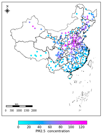
Figure 1.
PM2.5 concentrations (μg/m3) for the 295 cities in China during the winter of 2019–2020.
3. Methodology
3.1. Model of First-Order Binary Markov Chain
To assess the spatial connection of PM2.5 concentrations between different cities in China, we define a PM2.5 extreme for a specific city as the daily PM2.5 concentration exceeding the 80th percentile of PM2.5 concentrations in that city during the study period. A binary dataset is then obtained with the 80th percentile of daily PM2.5 concentrations as a threshold. In this binary PM2.5 network, when a PM2.5 extreme occurs on a particular day for a specific city, it is set as 1 for that day; otherwise it is set as 0. In this work, each node represents one city, and a network of 295 cities with daily PM2.5 concentrations results in a total of 43,365 city pairs.
Let (i, j) be a pair of distinct nodes, and (Xi, Xj) be binary variables representing the daily nonoccurrence (0) or occurrence (1) of a PM2.5 extreme for a pair of distinct nodes (i ≠ j). Here, {Xi, n} and {Xj, n} are the corresponding daily sequences for city i and j (n = 1, 2, …, N), respectively. For each node, the occurrence/nonoccurrence of a PM2.5 extreme is described by a two-state, first-order Markov chain [39,42]. For node i, the transition matrix of the Markov chain {Xi, n} is denoted by Pxi, which may be expressed as:
Here, and represent the conditional probabilities of transition from state 0 to state 0, and from state 0 to state 1, respectively. and represent the conditional probabilities of transition from state 1 to state 0, and from state 1 to state 1, respectively. Specifically, , and . In general, we use to illustrate the transition probability from state k at time n to state l at time n + 1 for node i, shown as:
where . Similarly, the transition matrix of daily sequence of {Xj, n} is denoted by Pxj, and . The transition probability represents the probability for node j transferring from state k at time n to state l at time n + 1, with .
Let be the marginal probability for node i, indicating the probability when Xi acquiring a specific value of l (), and is assumed to be constant for each n, as follows:
Similarly, the marginal probability for node j is denoted as , indicating the probability of Xj acquiring a specific value of l, as expressed as .
Let denote a pair of distinct nodes, with each node following a binary Markov chain (n = 1, 2, …, N). For a specific day (each n), there are four outcomes for each pair of nodes as follows , , and . The definitions of the four combinations are listed in Table 1. Here, the symbol of indicates the joint probability of the four possible outcomes of “00”, “01”, “10” and “11” for each pair of distinct nodes.

Table 1.
Definition of the four dependence types.
Here, represents the joint probability of the co-occurrence of a PM2.5 non-extreme for city i and a PM2.5 non-extreme for city j.
where represents the joint probability of combination “01” for a specific city pair (Xi, Xj), with a PM2.5 non-extreme for city i, while showing a PM2.5 extreme for city j at the same time.
Here, represents the joint probability of the co-occurrence of a PM2.5 extreme for city i, while PM2.5 non-extreme for city j.
Here, represents the joint probability of co-occurrence of a PM2.5 extreme and a PM2.5 extreme for a specific city pair (Xi, Xj) for all the daily sequences. The joint probabilities for the four outcomes of “00”, “01”, “10” and “11” are under the constraint of .
3.2. Method of Dependence Analysis
In this study, we define a hypothesis test for each pair of distinct nodes {Xi, n} and {Xj, n}, with the null hypothesis of independence and the alternative hypothesis of dependence for that pair of nodes. Based on the daily binarised PM2.5 concentration data, we calculate the sample estimates of the joint probabilities with respect to the four combinations of “00”, “01”, “10” and “11” for each city pair, as denoted by . Let indicate the joint probability under the null hypothesis of independence with a superscript I. At a significance level of α, we then calculate the confidence interval in hypothesis of independence, and compare with the confidence interval of in the hypothesis of independence. In order to calculate the confidence interval in the hypothesis of independence, we must first calculate the transition matrix for each node based on the theory of the Markov Chain. If the two Markov Chains {Xi, n} and {Xj, n} are independent of one another, the confidence interval of the probability of may be calculated via Monte Carlo simulations (Michele et al., 2020). Marginal probabilities for a specific pair of nodes are denoted by and with , and will be calculated in each Monte Carlo simulation. Under the null hypothesis of independence, the joint probability is the product of the marginal probabilities of each node, that is , with . The Monte Carlo confidence interval is indicated with MC superscript, with a lower and upper confidence interval of and , respectively. If , then the city pair (Xi, Xj) is considered independent with respect to combination.
In particular, we are interested in the dependence between each pair of chains with respect to the four combinations (), as shown in Equation (8):
In other words, we are focusing on when and where the joint probability of the “PM2.5 non-extreme and PM2.5 non-extreme”, “PM2.5 non-extreme and PM2.5 extreme”, “PM2.5 extreme and PM2.5 non-extreme” or the “PM2.5 extreme and PM2.5 extreme” event is greater than the probability pertaining to the independence case. Therefore, the dependence between the nodes of a binary PM2.5 network may be addressed through the pairwise analysis of the co-occurrences of the “PM2.5 non-extreme and PM2.5 non-extreme”, “PM2.5 non-extreme and PM2.5 extreme”, “PM2.5 extreme and PM2.5 non-extreme” or the “PM2.5 extreme and PM2.5 extreme” event, or the occurrence of these events with a lag time, which for most case studies was considered to be within ±3 days (Michele et al., 2020). In order to check the pairwise dependence with respect to the four combinations within each pair of nodes, we calculate the confidence internal of the probability via Monte Carlo experiments under the null hypothesis of independence. Here, a small significance level α = 0.5% is applied to avoid Type I errors. The confidence intervals of two independent, first-order binary Markov chains have been indicated by , and will be calculated with a sample size of N = 10,000 to allow a small error (less than 1%) in the estimation of confidence limits, as documented in a previous study (Michele et al., 2020). Figure 1 shows a network of the 295 cities located in China, with each node representing one city, and different colors represent the various PM2.5 concentrations in the 295 cities during the study period. Therefore, the dependence analysis of PM2.5 concentrations in the 295 Chinese cities could be achieved through the pairwise analysis of the co-occurrences of the four probabilities for all city pairs, considering a lag time in the range of ±3 days.
3.3. Procedure for Dependence Analysis
In this work, we define the following procedure to evaluate the dependence analysis of PM2.5 concentrations for the 295 Chinese cities in the winter of 2019–2020. The procedure is applied to each pair of nodes, and consists of the following steps: (1) Convert the original observed data into binary data, with 80% percentile as a threshold for each node. (2) For all 295 Chinese cities, every two cities are paired, and dependence analysis would be conducted for each pair of nodes. (3) Calculate the sample estimate of for each pair of nodes with respect to the four combinations (i.e., “00”, “01”, “10” and “11”), denoted as . (4) Under the null hypothesis of independence, calculate the respective confidence interval for each pair of nodes via Monte Carlo simulations under a significance level α = 0.5%. If , then the couple Xi, Xj is considered independent with respect to combination. Steps (1)–(4) represent a basic check for evaluating the independent pairs with respect to the four combinations, while the following steps represent an advanced check for dealing with doubt dependent couples. (5) If (or ), we check the behavior of the other combinations of (). For a specific pair of nodes, the sum of the four combinations (i.e., “00”, “01”, “10” and “11”) is one, and the increase of one would lead to the decrease of one or more . Thus, if and there is at least one other combination satisfying , then that pair of nodes of Xi and Xj is considered dependent with respect to combination . Similarly, if and there is at least one combination with , then the couple of Xi and Xj is judged dependent with respect to combination , as defined in the previous section. (6) For those couples of nodes which do not satisfy one combination larger than the upper 99.5% confidence interval, and another combination smaller than the lower 99.5% confidence interval at the same time, we consider a significance level of 1.5α = 0.75%, since the reduction of or could be not significant at a significance level of α. Meanwhile, if (or ) and (or ), then the pair of nodes Xi, Xj is considered dependent with respect to (or ), and the others are considered independent. (7) With a lag time in the range of ±3 days (lag = ±1 day, lag = ±2 days and lag = ±3 days), we recalculate the sample estimate of for each couple of nodes with each specific lag time for the four combinations, and obtain the dependent pairs of nodes following the steps described previously.
4. Results and Discussion
4.1. Overview of the Distribution of PM2.5 Concentration
The distribution of PM2.5 concentrations in the 295 Chinese cities was first analyzed, and the averaged PM2.5 concentrations in the winter period of 2019–2020 for each city were calculated based on the daily PM2.5 concentrations from the Chinese environmental monitoring stations. There were 67 cities with PM2.5 concentrations exceeding the national secondary standard limit in China (i.e., 75 μg/m3), accounting for approximately 22.71% of the 295 cities. The city that was most contaminated by PM2.5 was Anyang, followed by the cities of Xianyang, Yuncheng, Puyang, Linfen, Urumqi and Shijiazhuang. Specifically, the PM2.5 concentrations for the cities of Anyang, Xianyang, Yuncheng, Puyang, Linfen and Urumqi were 123.659 μg/m3, 112.275 μg/m3, 111.231 μg/m3, 109.978 μg/m3, 107.374 μg/m3 and 106.582 μg/m3, respectively. The highly contaminated cities were primarily located in Henan, Shanxi, Shaanxi, Hebei and Xinjiang areas. One reason for this was that there was less rainfall and convective activity in these cities; the other reason related to the presence of heavy industrial pollution or insufficient environmental protection. In contrast, the cities that were least contaminated by PM2.5 were Linzhi, Shannan, Sanya and Shigatse, with averaged PM2.5 concentrations of 5.187 μg/m3, 10 μg/m3, 12.978 μg/m3 and 13.253 μg/m3, respectively. The relatively lower scale of industrialization and urbanization contributed to the better atmospheric environment in these cities. In general, the contamination of PM2.5 in the North was more severe than the contamination in the South.
4.2. Dependence Analysis of PM2.5 Concentration
In this study, a network of 295 cities with daily PM2.5 concentrations resulted in a total of 43,365 pairs of nodes, and the method of dependence analysis was applied to each pair of nodes. As described previously, in order to test the dependence for each couple of nodes with a lag time in the range of ±3 days, the 80% percentile values of daily PM2.5 concentrations for each city were first calculated and set as the respective threshold for that city node. When the daily PM2.5 concentration exceeded the threshold, a PM2.5 extreme occurred for that day. Thus, the original daily PM2.5 concentrations were all converted to binary data. We then calculated the sample estimate of binary data at the time of lag 0, with respect to the four combinations of “00”, “01”, “10” and “11” for each city pair. For each city pair, the sum of the probabilities for the four outcomes of “00”, “01”, “10” and “11” were under the constraint of .
In particular, we were interested in whether the occurrence of a PM2.5 extreme in one city would cause co-occurrence of a PM2.5 extreme in another city. Here, we listed the time series trends of PM2.5 concentrations for two example city pairs with comparably small and high values of , as shown in Figure 2. For the city pair of “Shantou_Wulanchabu”, the PM2.5 extremes in Shantou and Wulanchabu never occurred at the same time, and the probabilities for the combinations of “00”, “01”, “10” and “11” were 0.626, 0.198, 0.176 and 0, respectively. By contrast, the city pair of “Anyang_Hebi” had a relatively high value of , and most of the PM2.5 extremes in Anyang and Hebi occurred at the same time. The probabilities of “00”, “01”, “10” and “11” combinations for the city pair of “Anyang_Hebi” were 0.791, 0.011, 0.011 and 0.187, respectively. The PM2.5 concentrations of Anyang and Hebi demonstrated similar increasing or decreasing trends during the study period, with the probabilities of “00” and “11” combinations accounting for 97.8% of all observation points.
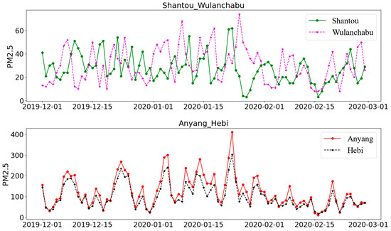
Figure 2.
PM2.5 concentrations (μg/m3) for the city pairs of “Shantou_Wulanchabu” and “Anyang_Hebi”.
To evaluate the distribution of probabilities for the four combinations of “00”, “01”, “10” and “11” for all city pairs, we calculated the number of city pairs with > 0.75, > 0.15, > 0.19 and > 0.19, respectively. The results showed 347 city pairs with greater than 0.75, and 175 city pairs with greater than 0.15. Meanwhile, for the 175 city pairs with greater than 0.15, their corresponding were all greater than 0.75. In addition, the results showed 558 city pairs with greater than 0.19, and 511 city pairs with probabilities of “10” greater than 0.19. As shown in Figure 3, > 0.75 or > 0.15 mainly occurred between cities which were relatively close to each other. In other words, high probabilities of “PM2.5 extreme and PM2.5 extreme” or “PM2.5 non-extreme and PM2.5 non-extreme” mainly occurred between nearby cities. The averaged distance of city pairs with > 0.75 was 154.773 km, while the average distance of > 0.15 was 121.105 km. In comparison, relatively higher probabilities for the combinations of “01” or “10” mainly occurred between cities which were far away from each other. That is, high probabilities of “PM2.5 extreme and PM2.5 non-extreme” mainly occurred with city pairs which were further away from each other. The averaged distance of city pairs with > 0.19 was 1685.011 km, while the average distance of city pairs with > 0.19 was 1750.809 km.
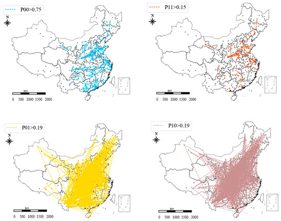
Figure 3.
Distributions of city pairs with P00 > 0.75, P11 > 0.15, P01 > 0.19 and P10 > 0.19, respectively.
After the sample estimate of each city pair that related to the four combinations of “00”, “01”, “10” and “11” was calculated, we then calculated the 99.5% confidence interval for each combination via Monte Carlo simulations. For the pairwise type of “00”, the sample estimates of were all within the 99.5% confidence interval, indicating all pairs of nodes were independent with respect to the “00” combination under a significance level of α = 0.5%. For the pairwise type of “01”, there were 79 pairs of nodes smaller than the lower 99.5% confidence intervals, and no pair larger than the upper 99.5% confidence interval. Thus, 43,286 pairs of nodes were independent with respect to the “01” combination. Regarding the “10” type, there were 75 pairs beyond the lower 99.5% confidence intervals, and 43,290 pairs of nodes were independent with respect to the “10” combination. As for the pairwise of the “11” type, there were 852 pairs smaller than the lower 99.5% confidence intervals, while 1813 pairs were larger than the upper 99.5% confidence intervals. Following step 5, 107 pairs of nodes showed to be dependent, which accounted for approximately 0.25% of total city pairs. In step 6, there were 47 couples with greater than and less than , while no couple satisfied less than and greater than . Therefore, 47 couples (0.11% of the total) proved to be dependent during step 6. The remaining couples were considered to be independent. Thus, for lag 0, 154 city pairs (0.36% of the total) proved to be dependent among 43,365 pairs, while the other 43,211 (99.64% of the total) were considered independent. The dependent couples were all type “11”. Considering a lag time of ±1 day, ±2 days and ±3 days, within which there were no more pairs of dependence, an indication of the choice of the max lag time of ±3 days would be sufficient. Figure 4 shows the distribution of the obtained 154 city pairs proved to be dependent with type “11”.
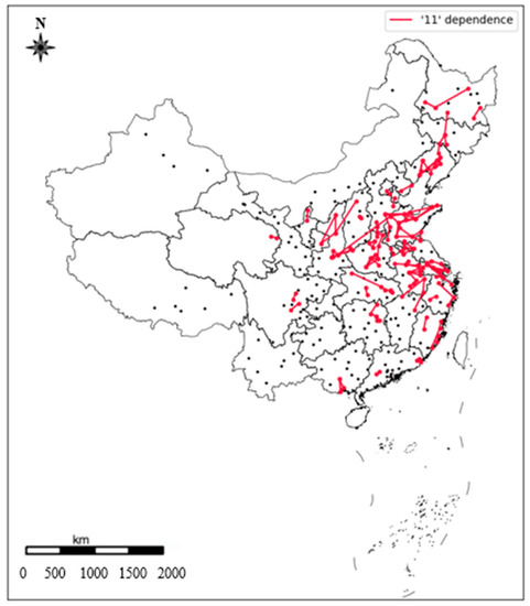
Figure 4.
Pairwise dependencies with a lag time in the range of (−3, +3) days, being only of “11” dependence type.
4.3. Distance of Dependent City Pairs
Based on the above analysis, we calculated a total of 154 pairs of cities with dependence type “11”. Dependence type “11” indicated that the occurrence of a PM2.5 extreme in one city was significantly associated with the co-occurrence of a PM2.5 extreme in the dependent city. When there was relatively high PM2.5 concentrations in one city, the dependent city also had relatively high PM2.5 concentrations compared to its other time. Generally, dependence type “11” primarily occurred between cities which were relatively close to each other, since PM2.5 air pollutants spread from one city to another, and it was easier for PM2.5 pollutants to reach nearby cities under favorable geographic conditions. On the other hand, the dependency weakened to be insignificant when the distance increased. Specifically, the dependent city pairs with the shortest distances were “Ezhou_Huanggang”, “Xiangtan_Zhuzhou”, “Xian_Xianyang”, “Yangzhou_Zhenjiang” and “Ezhou_Huangshi”, which were only 7.292 km, 18.670 km, 21.211 km, 22.712 km and 25.369 km away from each other within each city pair. Figure 5 illustrates the number of dependent city pairs with respect to various distance ranges. In general, there was a decreasing trend in the number of dependent city pairs as the distance increased. The results showed 81 dependent city pairs with distances less than 100 km, which accounted for 52.6% of the total dependent couples, and another 56 dependent pairs with distances between 100 km and 200 km. Therefore, the proportion of dependent pairs with a distance less than 200 km accounted for approximately 89.0% in total, while the results showed only 3.2% dependent couples with a distance greater than 300 km.
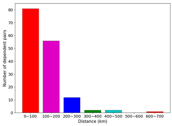
Figure 5.
Number of dependent city pairs for each distance range (colors of red, purple, blue, green, cyan, orange indicating the number of city pairs with distance ranges of 0–100 km, 100–200 km, 200–300 km, 300–400 km, 400–500 km, 600–700 km, respectively).
Interestingly, the results showed the PM2.5 extreme in one city may cause the co-occurrence of a PM2.5 extreme in another city hundreds of kilometers away. Table 2 illustrates the dependent city pairs with a distance greater than 200 km, and the dependent city pairs with the longest distance was “Dezhou_Weinan”. Even though Dezhou and Weinan were 697.218 km away from each other, the PM2.5 concentrations were able to influence each other, with a dependence type of “11”. The dependent city pair with the second longest distance was “Daqing_Hegang”, with a distance of 402.310 km. The respective distance within each dependent city pair for “Shuozhou_Yanan”, “Shiyan_Xiaogan” and “Qingyang_Yulin” was 402.272 km, 350.414 km and 341.317 km, respectively. Particularly, Figure 6 provides the time series trends of PM2.5 concentrations for each of the dependent city pairs “Dezhou_Weinan” and “Daqing_Hegang”. Both groups of the dependent city pairs of “Dezhou_Weinan” and “Daqing_Hegang” resulted in type “11” dependence. Under a significance level of 0.5%, when PM2.5 concentrations of Dezhou exceeded its threshold of 80% percentile, the city of Weinan also exceeded its threshold in general. Similarly, when PM2.5 extremes occurred in Daqing, PM2.5 extremes also occurred in the city of Hegang.
Table 2.
Dependent city pairs with a distance greater than 200 km.
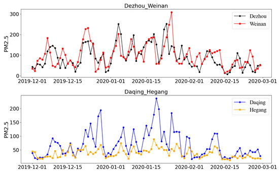
Figure 6.
Time series trends of PM2.5 (μg/m3) for the dependent pairs of “Dezhou_Weinan” and “Daqing_Hegang”.
4.4. Topography of Dependent City Pairs
City pairs with dependence type “11” mainly clustered in the North China Plain, the Northeast Plain, the Middle and Lower Yangtze Plain and the Fen-Wei Plain. The geographic conditions of the Plain areas were more conducive to the spread of PM2.5, which resulted in the mutual dependency of PM2.5 between cities. By contrast, the mountain topography was unfavorable for the formation of dependence type “11”. As shown in Table 2, those dependent city pairs with a distance greater than 200 km were all located in the Plain areas. Particularly, “Dezhou_Weinan”, “Shuozhou_Yanan”, “Qingyang_Yulin” and “Sanmenxia_Xianyang” were located in the Fen-Wei Plain. “Shiyan_Xiaogan”, “Xuancheng_Jiujiang”, “Hangzhou_Taizhou”, “Zhenjiang_Jiaxing” and “Huangshan_Yingtan” were located in the Middle and Lower Yangtze Plain. “Weihai_Weifang, “Dongying_Yantai”, “Weifang_Yantai” and “Hengshui_Binzhou” were located in the North China Plain, while “Daqing_Hegang”, “Huludao_Shenyang” and “Harbin_Changchun” were located in the Northeast Plain. Figure 7 provides the probabilities of the four combinations of “00”, “01”, “10” and “11” for the dependent city pairs located in Fen-Wei Plain at lag 0, where the estimate of was compared to the 99.5% confidence intervals. The examples shown in Figure 7 all exhibit dependence type “11” according to the procedure described previously. The green bars represent the upper and lower 99.5% confidence intervals obtained through Monte Carlo simulations. The black dots represent the sample estimate of . For the investigated pairs in Figure 7, were all within the 99.5% confidence intervals, and were all greater than 99.5% upper confidence intervals , while most of the and were smaller than the lower 99.5% confidence intervals , except for the city pairs of “Sanmenxia_Weinan” and “Weinan_Xianyang”. Considering a significance level of 1.5α, the of city-pair “Sanmenxia_Weinan” was smaller than the lower 99.25% confidence interval and was greater than the upper 99.5% confidence interval . Similarly, of “Weinan_Xianyang” was smaller than the lower 99.25% confidence interval and was greater than the upper 99.5% confidence interval . Thus, the city pairs of “Sanmenxia_Weinan” and “Weinan_Xianyang” were also considered to be dependent with respective to type “11”.
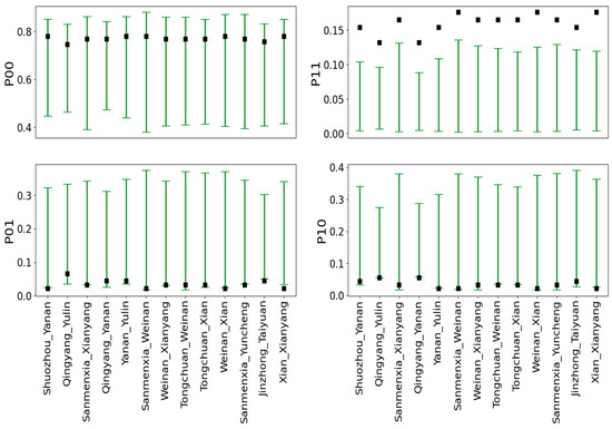
Figure 7.
Dependence analysis of some example city pairs located in Fen-Wei Plain.
The results showed that cities with high PM2.5 concentrations may not necessarily be dependent, while cities with low PM2.5 concentrations may instead be dependent. For example, the averaged PM2.5 concentrations of Turpan and Urumqi during the study period were 89.462 μg/m3 and 106.582 μg/m3, respectively. Although Turpan and Urumqi had high PM2.5 concentrations, there was no dependence between these two cities: they were independent. The possible reason for this was that the existence of the Tianshan Mountains hindered the spread of PM2.5 from one city to another, which further resulted in no dependence of PM2.5 concentrations in these cities. By comparison, even though the PM2.5 concentrations of city pairs “Shiyan_Xiaogan”, “Xuancheng_Jiujiang”, “Hangzhou_Taizhou”, “Zhenjiang_Jiaxing” and “Huangshan_Yingtan” were comparably low, there was significant dependence within each city couple. For instance, the corresponding PM2.5 concentrations of Hangzhou and Taizhou were 41.066 μg/m3 and 34.132 μg/m3, however, they formed a dependent city pair, indicating the PM2.5 of Hangzhou could impact that of Taizhou, and vice versa. This was primarily due to their location in the Plain area of the middle and lower reaches of the Yangtze River, even while they were distanced by more than 200 km. The Plain terrain conditions were more conducive to the transport of PM2.5, which resulted in a spatial dependence type “11” within the city pairs.
The co-occurrence of PM2.5 extremes were mainly located in the North China Plain, the Northeast Plain, etc. Relatively high coal consumption and national steel production has led to the poor air quality in the North China Plain and Northeast China Plain areas (Fan et al., 2020; He et al., 2021). The large proportion of land for construction and population density, and the relatively small percentage of forestland, has contributed to the PM2.5 pollution in the Yangtze River delta [23]. The impact of meteorology on PM2.5 contamination was complicated with spatial variations in China. Specifically, relative humidity and the lifted index exerted a strong positive influence on PM2.5 in Central China, and elevation mainly influenced PM2.5 in the Beijing-Tianjin-Hebei region and the Sichuan basin [19]. The relative humidity was positively correlated with the PM2.5 concentration in North China and Urumqi, and the positive relation was stronger in winter, while surface pressure had a positive relationship with PM2.5 in northeast China and mid-south China [33]. In addition, large-scale atmospheric circulations also exerted certain influences on the regional PM2.5 pollution [43]. Generally, the combination of the stable boundary layer, frequent air stagnation and near-surface horizontal convergence has exacerbated the wintertime PM2.5 pollution in the Beijing-Tianjin-Hebei region [43]. Different kinds of atmospheric internal boundaries have impacted PM2.5 pollution in the North China Plain, and the frontal category was recognized as the most polluted type during the formation–maintenance stage [44].
4.5. Impact of Significance Level
Traditionally, a small value of significance level α is recommended for a hypothesis test to avoid a Type I error. Significance level α represents the probability of rejecting a true null hypothesis. In other words, the significance level represents the probability of misclassifying independent city pairs as dependent in this study. To test the sensitivity and the corresponding influence of significance level α on the dependence analysis of PM2.5 concentrations in the 295 Chinese cities, three significance levels were primarily investigated (i.e., α = 0.5%, α = 1% and α = 2%). A total of 154, 204 and 555 city pairs were calculated as dependent with type “11” for the significance levels of 0.5%, 1% and 2%, respectively. As we expect, the confidence intervals of the hypothesis test for independence shrink with an increase in the significance level, which would further lead to additional dependent city pairs. Figure 8 shows the distribution of dependent city pairs under different significance levels of 0.5%, 1% and 2%, and the number of dependent city pairs for these three categories. As may be seen from Figure 8, the number of dependent city pairs increased as significance level α increased. In addition, the averaged distances of the dependent pairs for significance levels of 0.5%, 1% and 2% were 112.338 km, 124.123 km and 201.809 km, respectively. An increasing trend was seen in the averaged distance of dependent city pairs as the significance level increased. The dependence analysis of PM2.5 concentrations in the 295 Chinese cities was found to be sensitive to the significance level selected. In this study, a significance level of 0.5% was recommended for dependence analysis.
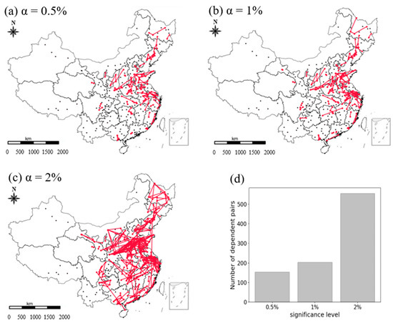
Figure 8.
Distribution of dependent city pairs under different significance levels: (a) α = 0.5%; (b) α = 1%; (c) α = 2%; and (d) histogram of number of dependent city pairs for three categories.
5. Conclusions
The spatial distribution of PM2.5 concentrations in the 295 Chinese cities, during the winter period of 2019–2020, showed that the PM2.5 concentrations of 67 cities exceeded the national secondary standard limit in China, accounting for approximately 22.71% of all the 295 cities. The cities which were mostly contaminated were mainly located in Henan, Hebei, Shanxi, Shaanxi and Xinjiang. The heavy PM2.5 pollutions in these areas are mainly due to industrial pollution, unreasonable energy structure and the unfavorable weather conditions (i.e., less rainfall, dry weather, etc). By contrast, relatively lower-scale industrialization and urbanization contributed to the good air quality of the cities of Linzhi, Shannan, Sanya and Shigatse.
In this study, we applied a methodology of dependence analysis to analyze the daily concentrations of PM2.5 air pollutants in the network of 295 cities in China, during the studied winter period. We also developed a procedure to efficiently evaluate the dependent city pairs within the binary PM2.5 network. Based on the dependence analysis, a total of 154 city pairs were identified with respect to the dependence type “11”, indicating that when there were relatively high PM2.5 concentrations in one city (PM2.5 extremes), there were also PM2.5 extremes for the dependent city. Furthermore, this dependence mainly occurred between cities which were relatively close to one another, as PM2.5 may reach nearby cities more easily under favorable geographic conditions. As the distance increased, the dependence weakened to be insignificant. In total, the distances between 89.0% of the dependent city pairs were less than 200 km. A PM2.5 extreme in one city may cause the co-occurrence of a PM2.5 extreme in another city hundreds of kilometers away. The longest distance of the dependent city pair was 697.218 km.
The dependent city pairs mainly clustered in the North China Plain, the Northeast Plain, the Middle and Lower Yangtze Plain and the Fen-Wei Plain. The topography structure may help explain the location of spatial dependence in PM2.5 concentrations to a certain extent. The geographical conditions of the Plain areas were more conducive to the spread of PM2.5, while the mountain topography was unfavorable for the formation of PM2.5 dependencies between different cities. Under favorable geographic conditions, the PM2.5 in one city could impact the PM2.5 in another city, even though they were several hundreds of kilometers away. The dependent city pairs with distances greater than 200 km were all located in Plain areas. Interestingly, some cities with high PM2.5 concentrations were not dependent, while other cities with relatively low PM2.5 concentrations were dependent. For instance, the PM2.5 concentrations in Turpan and Urumqi were very high, however, they were not dependent, since the existence of the Tianshan Mountains has hindered the migration of PM2.5 between these cities. By contrast, there were several city couples with low PM2.5 concentrations, yet they were dependent. For example, the PM2.5 concentrations of Hangzhou and Taizhou were relatively low compared to that of the cities in Xinjiang province, yet they were dependent. This was primarily due to their location in the Plain areas of the middle and lower reaches of the Yangtze River, and the topography of the Plain area benefited the transport of PM2.5 from one city to another, which led to the dependence of PM2.5 in these cities. In addition, the dependence analysis of PM2.5 concentrations in the 295 Chinese cities was found to be sensitive to the significance level selected. As the significance level increased, the number of dependent city pairs increased, and the averaged distance of dependent city pairs also increased. To avoid Type I errors, a small value of significance level α = 0.5% was recommended in this work.
The methodology developed in this study may help identify the spatial dependence of PM2.5 concentrations over the 295 cities located in China. Pairwise dependence findings in this research helped us identify the geographic areas where compound high-contamination PM2.5 disasters may occur. Understanding the spatial dependence of air pollution is conducive to government decision-making and the prevention of large-scale air pollution; for instance, the government could relocate those heavily polluted industries away from the highly contaminated Plain areas. This study innovatively developed a quantitative way to measure the connections between PM2.5 concentrations in various Chinese cities. Identifying the connections between PM2.5 in different cities is crucial in environmental studies, including the classification of air quality or air quality estimation by interpolation in China, and this contribution is different from previous studies in the atmosphere and the environment. However, there were some limitations. Firstly, the study period spanned only the winter period due to the availability of continuous-time data, which may result in certain missing information. The possible extension of this work will include the dependence analysis of city pairs for a longer period in the future. Secondly, this study mainly focused on the dependence analysis of PM2.5; the application of this methodology to other air pollutants will be conducted in the future. Furthermore, the impact of climate and atmospheric synoptic scale circulation upon the concentration of PM2.5 will be conducted in the future.
Author Contributions
Conceptualization, C.B.; Formal analysis, P.Y.; Writing–original draft, C.B. All authors have read and agreed to the published version of the manuscript.
Funding
This research was funded by National Key R&D Program of China (2021YFC3001000), the Guangdong Provincial Natural Science Foundation Project (No. 2020A1515010437).
Institutional Review Board Statement
Not applicable.
Informed Consent Statement
Not applicable.
Data Availability Statement
Not applicable.
Conflicts of Interest
The authors declare no competing interest.
References
- Lei, Y.; Davies, G.M.; Jin, H.; Tian, G.; Kim, G. Scale-dependent effects of urban greenspace on particulate matter air pollution. Urban For. Urban Green. 2021, 61, 127089. [Google Scholar] [CrossRef]
- Wang, J.; Zhang, L.; Niu, X.; Liu, Z. Effects of PM2.5 on health and economic loss: Evidence from Beijing-Tianjin-Hebei region of China. J. Clean. Prod. 2020, 257, 120605. [Google Scholar] [CrossRef]
- Jin, H.; Chen, X.; Zhong, R.; Liu, M. Influence and prediction of PM2.5 through multiple environmental variables in China. Sci. Total Environ. 2022, 849, 157910. [Google Scholar] [CrossRef] [PubMed]
- Geng, G.; Zheng, Y.; Zhang, Q.; Xue, T.; Zhao, H.; Tong, D.; Zheng, B.; Li, M.; Liu, F.; Hong, C.; et al. Drivers of PM2.5 air pollution deaths in China 2002–2017. Nat. Geosci. 2021, 14, 645–650. [Google Scholar] [CrossRef]
- Schwartz, J.; Wei, Y.; Yitshak-Sade, M.; Di, Q.; Dominici, F.; Zanobetti, A. A national difference in difference analysis of the effect of PM2.5 on annual death rates. Environ. Res. 2021, 194, 110649. [Google Scholar] [CrossRef]
- Chu, M.; Sun, C.; Chen, W.; Jin, G.; Gong, J.; Zhu, M.; Yuan, J.; Dai, J.; Wang, M.; Pan, Y. Personal exposure to PM2.5, genetic variants and DNA damage: A multi-center population-based study in Chinese. Toxicol. Lett. 2015, 235, 172–178. [Google Scholar] [CrossRef]
- Guo, X.; Lin, Y.; Lin, Y.; Zhong, Y.; Yu, H.; Huang, Y.; Yang, J.; Cai, Y.; Liu, F.; Li, Y.; et al. PM2.5 induces pulmonary microvascular injury in COPD via METTL16-mediated m6A modification. Environ. Pollut. 2022, 303, 119115. [Google Scholar] [CrossRef]
- Liang, X.; Chen, J.; An, X.; Liu, F.; Liang, F.; Tang, X.; Qu, P. The impact of PM2.5 on children’s blood pressure growth curves: A prospective cohort study. Environ. Intern. 2022, 158, 107012. [Google Scholar] [CrossRef]
- Khanna, I.; Khare, M.; Gargava, P.; Khan, A.A. Effect of PM2.5 chemical constituents on atmospheric visibility impairment. J. Air Waste Manag. Assoc. 2018, 68, 5. [Google Scholar] [CrossRef]
- Fang, X.; Fan, Q.; Liao, Z.; Xie, J.; Xu, X.; Fan, S. Spatial-temporal characteristics of the air quality in the Guangdong-HongKong-Macau Greater Bay Area of China during 2015–2017. Atmos. Environ. 2019, 210, 14–34. [Google Scholar] [CrossRef]
- Zhang, L.; An, J.; Liu, M.; Li, Z.; Liu, Y.; Tao, L.; Liu, X.; Zhang, F.; Zheng, D.; Gao, Q.; et al. Spatiotemporal variations and influencing factors of PM2.5 concentrations in Beijing, China. Environ. Pollut. 2020, 262, 114276. [Google Scholar] [CrossRef] [PubMed]
- He, Q.; Zhang, M.; Song, Y.; Huang, B. Spatiotemporal assessment of PM2.5 concentrations and exposure in China from 2013 to 2017 using satellite-derived data. J. Clean. Prod. 2021, 286, 124965. [Google Scholar] [CrossRef]
- Jin, H.; Zhong, R.; Liu, M.; Ye, C.; Chen, X. Spatiotemporal distribution characteristics of PM2.5 concentration in China from 2000 to 2018 and its impact on population. J. Environ. Manag. 2022, 323, 116273. [Google Scholar] [CrossRef] [PubMed]
- Gu, Y.; Wong, T.W.; Dong, G.H.; Ho, K.F.; Yang, Y.; Yim, S.H.L. Impacts of sectoral emissions in China and the implications: Air quality, public health, crop production, and economic costs. Environ. Res. Lett. 2018, 13, 084008. [Google Scholar] [CrossRef]
- Liu, Q.; Zhang, Z.; Shao, C.; Zhao, R.; Guan, Y.; Chen, C. Spatio-temporal variation and driving factors analysis of PM2.5 health risks in Chinese cities. Ecol. Indic. 2021, 129, 107937. [Google Scholar] [CrossRef]
- Wang, X.; Zhong, S.; Bian, X.; Yu, L. Impact of 2015–2016 EI Nino and 2017–2018 La Nina on PM2.5 concentrations across China. Atmos. Environ. 2019, 208, 61–73. [Google Scholar] [CrossRef]
- Xu, H.; Chen, H. Impact of urban morphology on the spatial and temporal distribution of PM2.5 concentration: A numerical simulation with WRF/CMAQ model in Wuhan, China. J. Environ. Manag. 2021, 290, 222427. [Google Scholar] [CrossRef]
- Xu, W.; Jin, X.; Liu, M.; Ma, Z.; Wang, Q.; Zhou, Y. Analysis of spatiotemporal variation of PM2.5 and its relationship to land use in China. Atmos. Pollut. Res. 2021, 12, 101151. [Google Scholar] [CrossRef]
- Yang, Q.; Yuan, Q.; Yue, L.; Li, T. Investigation of the spatially varying relationships of PM2.5 with meteorology, topography, and emissions over China in 2015 by using modified geographically weighted regression. Environ. Pollut. 2020, 262, 114257. [Google Scholar] [CrossRef]
- Hao, Y.; Liu, Y.M. The influential factors of urban PM2.5 concentrations in China: A spatial econometric analysis. J. Clean. Prod. 2016, 112, 1443–1453. [Google Scholar] [CrossRef]
- Lim, C.H.; Ryu, J.; Choi, Y.; Jeon, S.W.; Lee, W.K. Understanding global PM2.5 concentrations and their drivers in recent decades (1998–2016). Environ. Intern. 2020, 144, 106011. [Google Scholar] [CrossRef] [PubMed]
- Wu, W.; Zhang, M.; Ding, Y. Exploring the effect of economic and environment factors on PM2.5 concentration: A case study of the Beijing-Tianjin-Hebei region. J. Environ. Manag. 2020, 268, 110703. [Google Scholar] [CrossRef]
- Xu, G.; Ren, X.; Xiong, K.; Li, L.; Bi, X.; Wu, Q. Analysis of the driving factors of PM2.5 concentration in the air: A case study of the Yangtze River Delta, China. Ecol. Indic. 2020, 110, 105889. [Google Scholar] [CrossRef]
- Zhang, Y.; Shuai, C.; Bian, J.; Chen, X.; Wu, Y.; Shen, L. Socioeconomic factors of PM2.5 concentrations in 152 Chinese cities: Decomposition analysis using LMDI. J. Clean. Prod. 2019, 218, 96–107. [Google Scholar] [CrossRef]
- Li, X.; Feng, Y.J.; Liang, H.Y. The impact of meteorological factors on PM2.5 variations in Hong Kong. Earth Environ. Sci. 2017, 78, 012003. [Google Scholar] [CrossRef]
- Pan, S.; Du, S.; Wang, X.; Zhang, X.; Xia, L.; Liu, J.; Pei, F. Analysis and interpretation of the particulate matter (PM10 and PM2.5) concentrations at the subway stations in Beijing, China. Sustain. Cities Soc. 2019, 45, 366–377. [Google Scholar] [CrossRef]
- Yan, D.; Lei, Y.; Shi, Y.; Zhu, Q.; Li, L.; Zhang, Z. Evolution of the spatiotemporal pattern of PM2.5 concentrations in China—A case study from the Beijing-Tianjin-Hebei region. Atmos. Environ. 2018, 183, 225–233. [Google Scholar] [CrossRef]
- Liu, Y.; Shi, G.; Zhan, Y.; Zhou, L.; Yang, F. Characteristics of PM2.5 spatial distribution and influencing meteorological conditions in Sichuan Basin, southwestern China. Atmos. Environ. 2021, 253, 118364. [Google Scholar] [CrossRef]
- Fan, H.; Zhao, C.; Yang, Y. A comprehensive analysis of the spatio-temporal variation of urban air pollution in China during 2014–2018. Atmos. Environ. 2020, 220, 117066. [Google Scholar] [CrossRef]
- Hu, M.; Wang, Y.; Wang, S.; Jiao, M.; Huang, G.; Xia, B. Spatial-temporal heterogeneity of air pollution and its relationship with meteorological factors in the Pearl River delta, China. Atmos. Environ. 2021, 254, 118415. [Google Scholar] [CrossRef]
- Wen, X.; Zhang, P.; Liu, D. Spatiotemporal variations and influencing factors analysis of PM2.5 concentrations in Jilin province, Northeast China. Chin. Geo. Sci. 2018, 28, 810–822. [Google Scholar] [CrossRef]
- Yang, Q.; Yuan, Q.; Li, T.; Shen, H.; Zhang, L. The relationships between PM2.5 and meteorological factors in China: Seasonal and regional variations. Int. J. Environ. Res. Public Health 2017, 14, 1510. [Google Scholar] [CrossRef] [PubMed]
- Chen, Z.; Chen, D.; Xie, X.; Cai, J.; Zhuang, Y.; Cheng, N.; He, B.; Gao, B. Spatial self-aggregation effects and national division of city-level PM2.5 concentrations in China based on spatiotemporal clustering. J. Clean. Prod. 2019, 207, 875–881. [Google Scholar] [CrossRef]
- Liu, L.; Duan, Y.; Li, L.; Xu, L.; Yang, Y. Spatiotemporal trends of PM2.5 concentrations and typical regional pollutant transport during 2015–2018 in China. Urban Clim. 2020, 34, 100710. [Google Scholar] [CrossRef]
- Luo, J.; Du, P.; Samat, A.; Xia, J.; Che, M.; Xue, Z. Spatiotemporal pattern of PM2.5 concentrations in mainland China and analysis of its influencing factors using geographically weighted regression. Sci. Rep. 2017, 7, 40607. [Google Scholar] [CrossRef] [PubMed]
- Zhou, D.; Gozolchiani, A.; Ashkenazy, Y.; Havlin, S. Teleconnection paths via climate network direct link detection. Phys. Rev. Lett. 2015, 115, 268501. [Google Scholar] [CrossRef]
- Boers, N.; Goswami, B.; Rheinwalt, A.; Bookhagen, B.; Hoskins, B.; Kurths, J. Complex networks reveal global pattern of extreme-rainfall teleconnections. Nature 2019, 566, 373. [Google Scholar] [CrossRef] [PubMed]
- Michele, C.D.; Meroni, V.; Rahimi, L.; Deidda, C.; Ghezzi, A. Dependence types in a binarized precipitation network. Geophys. Res. Lett. 2020, 47, 23. [Google Scholar] [CrossRef]
- Tsonis, A.A.; Swanson, K.L.; Roebber, P.J. What do networks have to do with climate? Bull. Am. Meteorol. Soc. 2006, 87, 585. [Google Scholar] [CrossRef]
- Tsonis, A.A.; Swanson, K.L. Topology and predictability of EI Nino and La Nina networks. Phys. Rev. Lett. 2008, 100, 228502. [Google Scholar] [CrossRef]
- Zhao, S.; Yu, Y.; Yin, D.; He, J.; Liu, N.; Qu, J.; Xiao, J. Annual and diurnal variations of gaseous and particulate pollutants in 31 provincial capital cities based on in situ air quality monitoring data from China National Environmental Monitoring Center. Environ. Int. 2016, 86, 92–106. [Google Scholar] [CrossRef] [PubMed]
- Wilks, D.S. Statistical Methods in the Atmospheric Sciences; Elsevier Academic Press Publications: San Diego, CA, USA, 2020. [Google Scholar] [CrossRef]
- Wang, X.; Zhang, R. Effects of atmospheric circulations on the interannual variation in PM2.5 concentrations over the Beijing-Tianjin-Hebei region in 2013–2018. Atmos. Chem. Phys. 2020, 20, 7667–7682. [Google Scholar] [CrossRef]
- Jin, X.; Cai, X.; Yu, M.; Wang, X.; Song, Y.; Wang, X.; Zhang, H.; Zhu, T. Regional PM2.5 pollution confined by atmospheric internal boundaries in the North China Plain: Analysis based on surface observations. Sci. Total Environ. 2022, 841, 156728. [Google Scholar] [CrossRef] [PubMed]


Publisher’s Note: MDPI stays neutral with regard to jurisdictional claims in published maps and institutional affiliations. |
© 2022 by the authors. Licensee MDPI, Basel, Switzerland. This article is an open access article distributed under the terms and conditions of the Creative Commons Attribution (CC BY) license (https://creativecommons.org/licenses/by/4.0/).