Abstract
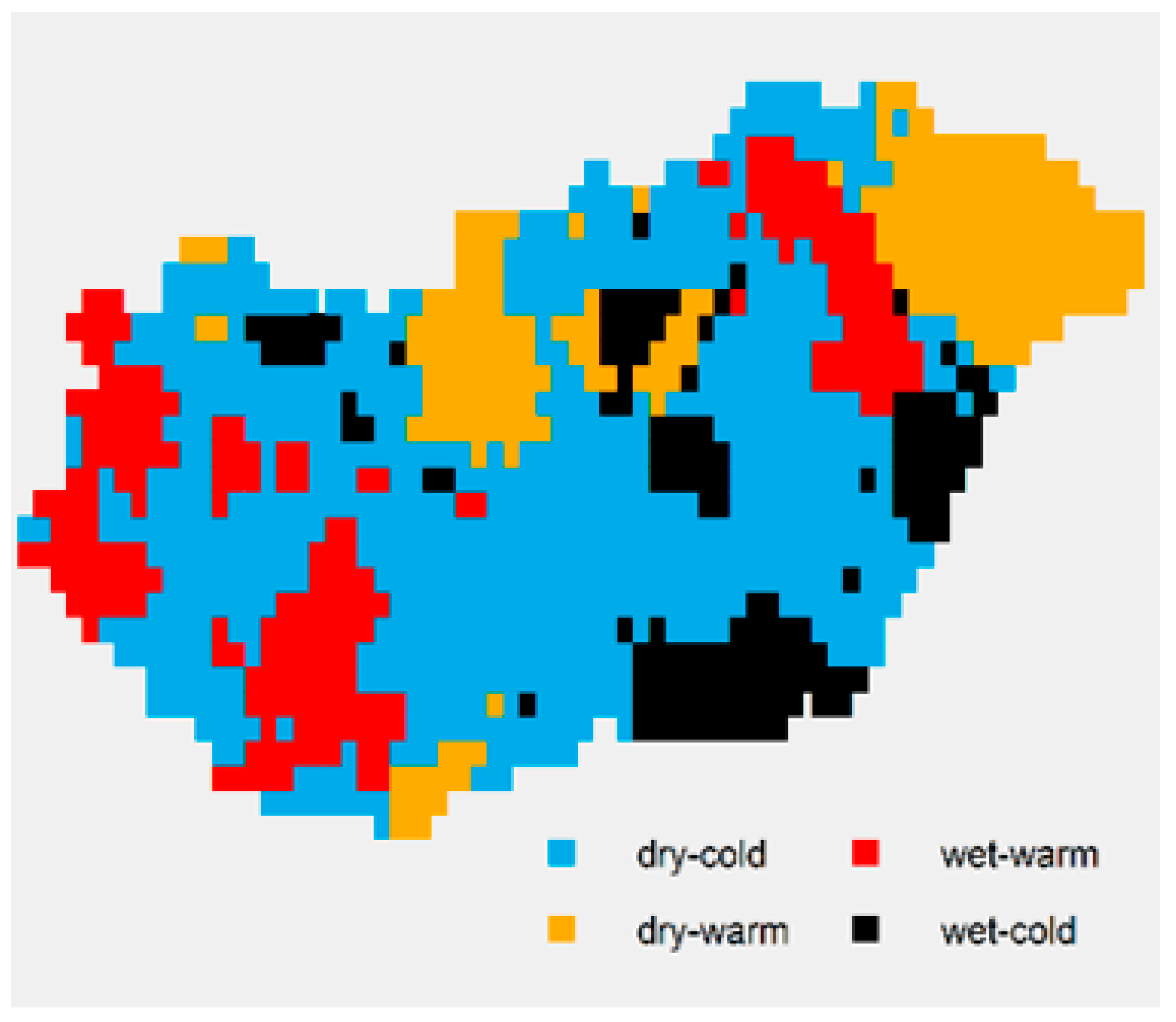
In addition to the one-dimensional mathematical statistical methods used to study the climate and its possible variations, the study of several elements together is also worthwhile. Here, a combined analysis of precipitation and temperature time series was performed using the norm method based on the probability distribution of the elements. This means, schematically speaking, that each component was transformed into a standard normal distribution so that no element was dominant. The transformed components were sorted into a vector, the inverse of the correlation matrix was determined and the resulting norm was calculated. Where this norm was at the maximum, the extreme vector, in this case the extreme month, was found. In this paper, we presented the results obtained from a joint analysis of the monthly precipitation and temperature time series for the whole territory of Hungary over the period 1871–2020. To do this, multidimensional statistical tests that allowed the detection of climate change were defined. In the present analysis, we restricted ourselves to two-dimensional analyses. The results showed that none of the tests could detect two-dimensional climate change on a spatial average for the months of January, April, July and December, while all the statistical tests used indicated a clear change in the months of March and August. As for the other months, one or two, but not necessarily all tests, showed climate change in two dimensions.
1. Introduction
One-dimensional extreme value theory and its practical applications are widely used and provide a very rich literature [1,2,3,4]. Since the mid-20th century, the study of extremes has also come to the fore in climate change research. In many cases, it has been observed that no change in the average can be detected, while trends in the intensity and frequency of extremes do give indications of a changing climate [5,6]. The magnitude and frequency of many climatic extremes (extreme indices) have changed significantly over the last few decades. The key question, however, is how an extreme meteorological event at a given geographical location and time is defined. For example, in Hungary, a prolonged drought is an extreme event, whereas in desert areas, daily precipitation of more than 10–15 mm is more likely to be an extreme event.
The basic mode of any approach to the study of climatic extremes is either the analysis of time series of extreme climatic elements [7,8,9] or the analysis of extremes in climate time series [10]. In the latter case, the extreme is usually taken to mean the maximum or minimum value of a given climate element over a given period. In one dimension, the interpretation of an extreme is therefore clear: the timing of its occurrence is immediately apparent, and a statistical analysis of the extreme also makes it possible to clarify whether the null hypothesis of an identical distribution of the elements of the time series is plausible or not. The examination of extreme values can therefore be an effective tool for detecting possible climate change, and extreme periods can be clearly identified from the times of the occurrence of the maximum and minimum values.
It follows naturally, then, to question whether, if certain climate elements are considered together, it is possible or even meaningful to talk about “extreme values” for a given multidimensional time series. In the multidimensional case, extremes can no longer be interpreted simply in terms of maximum and minimum values, but rather as combinations of elements occurring, some of which we might take for granted and some that seem unusual to us. The latter can also be conceived of as cases in which the elements individually do not exhibit any characteristic or value out of the ordinary, but their occurrence together can be considered an extreme phenomenon. Indeed, it can be argued that the study of such extremes is a more effective tool for studying and characterising climate change than simply one-dimensional cases [10,11,12].
In Section 3, a combined analysis of the precipitation and temperature data series is presented, performed using the norm method based on the probability distribution of the elements. This method was developed by Tamás Szentimrey [10,12], and its application has so far only been published as applied to meteorological elements on annual and seasonal scales [12]. First applied to monthly series, in the present study, both one-dimensional and two-dimensional climate variations were presented for each month. The main question to be answered is the same as for higher dimensionality: which vector should be considered extreme? Our aim was to identify extreme events in the multidimensional domain and to determine any possible multidimensional climate variability. Thus, a method was applied that was both mathematically correct and yet could be effectively applied in practice. In this paper, the results obtained so far and their application to climate time series are presented. This investigation was restricted to the Carpathian Basin, and within this basin the one- and two-dimensional monthly extremes of the Hungarian regions were examined. Monthly values of mean temperature and precipitation sums for the period 1871–2020 were used. The notion of multidimensional extremes was defined, and one- and two-dimensional extremes were identified. We showed which vector in each month may be considered extreme in terms of national averages. In addition, we also performed a spatial analysis for the whole of Hungary, i.e., we showed which vector was considered extreme in each geographical location (0.1° × 0.1° resolution) for the period 1871–2020.
Other multivariate extreme value methods can be found in the literature. In general, the main difficulties are related to the different probability distributions of the variables and the handling of the stochastic relationship between them [13,14,15,16]. One possible procedure is to estimate the joint probability density function using the kernel function method [17,18,19,20] and look for extreme values on the basis of this function. More recently, there have been several examples of copula fitting being employed [21,22,23,24]. The copula calculation has come to the fore in the context of the realization of the loss function, and thus the evaluation of risk as an economic and social interest [4]. Its popularity is also due to the fact that most statistical programs include a copula package, which greatly simplifies its application [25]. In the multivariate case, the copula function characterizes the relationship between the marginal distribution of each component and the joint distribution function. The copula method is used to examine extreme indices [26], such as the length and intensity of a dry period [27]. Since this method was developed to estimate the risk (or design value or return value) of a multidimensional extreme meteorological event, the question of which vector is considered extreme does not fall within its purview [28]. Therefore, in the context of the question to be addressed, the ‘norm method’ does not bear comparison to the copula method; they were designed to deal with different issues.
2. Materials and Methods
2.1. Creation of a Representative Database
The study of climate and its possible changes should only be carried out on the basis of a high-quality climatological database. First and foremost, therefore, what is needed is high-quality data: a database that is representative in both space and time.
The analysis of national temperature and precipitation extremes presented here was based on measurements available in the OMSZ (Hungarian Meteorological Service) climate database. The fact that changes in the measurement environment cause inhomogeneities in the station data series needs to be taken into account [29]. This can be caused by moving stations to a location with a different climate, or changing the environment of the station, the methodology or also the instrumentation. The station data series was homogenized, any data gaps were filled and data quality control was performed using the MASH (Multiple Analysis of Series of Homogenization) [30] software at the Climate Department of the OMSZ [31,32].
To ensure spatial representativity, estimates were provided for geographical locations where no measurements were made, as the station network density is not uniform in the Carpathian Basin. Spatial interpolation is a mathematical procedure that determines the value of a state indicator (meteorological element) at an arbitrary point based on known data observed at neighbouring locations [33,34,35]. For this task, the MISH (Meteorological Interpolation based on Surface Homogenized Data Basis) software was developed at the Climate Department of the OMSZ [31]. The most common and best-known interpolation methods in the earth sciences are geostatistical methods [33,34,35]. Their application in the field of meteorology does not yield good results, but in many cases, it is the only viable approach in the earth sciences. Meteorology, on the other hand, is in the fortunate position of having long data series, and thus much more information is available for any given region than in other sciences. The information contained in the long data series produced by MASH is used by the MISH software for modelling the climate statistical parameters, allowing us to give a much better estimate of a point where no measurements have been previously made than in the case of an estimate of stochastic relationships or spatial trends based on a snapshot. For this reason, the homogenised series were interpolated onto a dense spatial grid with a spatial resolution of 0.1°, covering the whole of Hungary, using the MISH system, as was also done for CarpatClim [36,37] by the participating countries.
Using MASH and MISH, it is possible to create a high-quality spatially and temporally representative database. A common feature of both software packages is that they take into account the probability distribution of the given element, allowing a choice between an additive or multiplicative model [30,34]. Unfortunately, this is not the case for most homogenization and interpolation software, which uses an additive model regardless of the probability distribution, as in the case of a normal distribution [38].
2.2. Data
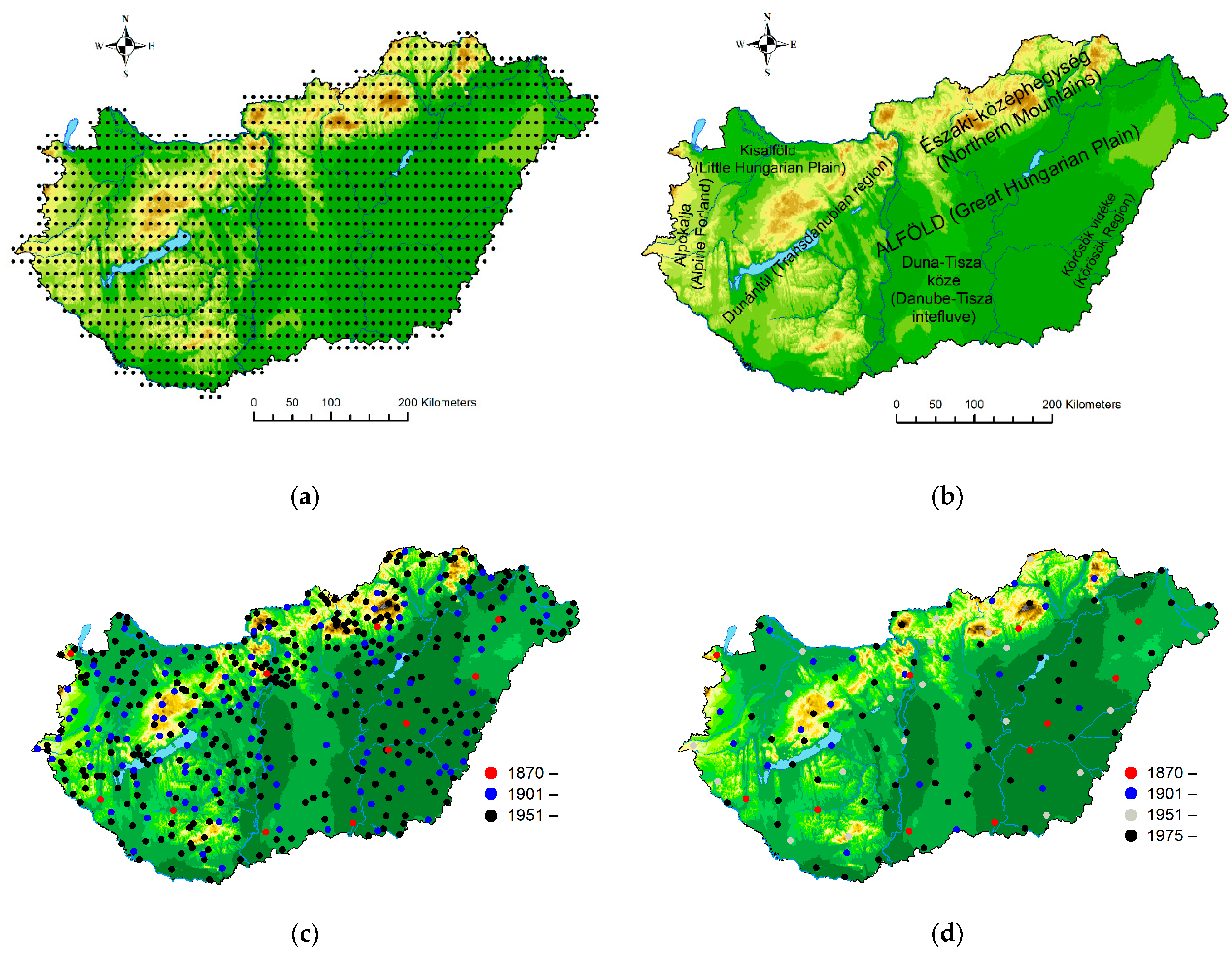
Just as the results of future projections should not be derived from the results of global models [39], a regional database is better suited to understanding the past and present than an observational database from a sparse network of stations [40]. The database, updated annually by the Climate Department of the OMSZ, not only provides input to regional climate models, but also helps in the better understanding of the climate of present and past centuries. To study the extremes, series for the daily mean temperature and precipitation sum for the period 1871–2020 were homogenized by MASH and interpolated using MISH software. The data series were constructed by using the most-available station data series at each time point for homogenization and then for interpolation [41] (Figure 1a–d). To ensure spatial representativity, the values were interpolated onto a dense regular grid (0.1 × 0.1° resolution) (Figure 1a), and thus the climate and its extremes over the whole country could be reported on. The resulting station and grid point database is called the HuClim database [42]. The names of the landscapes used in the article can be found in Figure 1b.

Figure 1.
(a) Spatial location of the grid points (EPSG:4326: WGS 84). (b) The Hungarian and English names of the landscapes. (c) Location of the stations in the case of precipitation. (d) Location of the stations in case of temperature.
3. Norm Method Based on Probability Distribution
In the following subsections, the norm method based on the probability distribution of the elements is presented, covering the main concepts necessary to understand the analyses and results reported here. The application of the method is considered appropriate when several interdependent meteorological elements and parameters are to be studied and analysed together. A more detailed description can be found in [12]. The aim was to present a mathematically and practically acceptable and efficient method for the study of multidimensional climate extremes.
3.1. Mathematical Model in General Case
Multidimensional time series:
These are totally independent and identically distributed probability vector variables.
The distribution functions of the components:
The vector of expectations:
The vector of standard deviations:
3.2. “Basic” Questions and Problems
The joint examination of the vector components may be efficient for the characterization of extreme events. In general, the main difficulties are connected to their different probability distributions and the handling of the stochastic relationship between them.
In this connection, two questions need to be addressed:
- –
- Which vector variable may be considered extreme?
- –
- How is it possible to test the null hypothesis of the identical distribution of the vector variables on the basis of the analysis of extremes?
These two questions will be answered in the following chapters.
3.3. Transformation of the Vector Components
To ensure that no component was dominant in the analysis of the vector variable, each component was transformed to the same distribution. In this case, the standard normal distribution was chosen as the identical distribution [10,12].
Let the meteorological variables in the given period be:
The standard normal series is:
where is the distribution function of is the inverse of the standard normal distribution function.
If the components were examined separately, the use of the variables or would be equivalent in respect of the degree of extremity.
It can be seen that the is extreme, i.e., an extreme realization, if and only if is extreme [12].
3.4. Definition of the Multidimensional Extreme
Let = be the vector variable under examination, now with transformed components.
Then the joint extreme index is:
where R is the correlation matrix of .
Based on the above norm:
and are extremes, if = (t = 1,2,……, n)
It can be seen that if the joint distribution of the components of is normal, then its density function is a strictly monotonic decreasing function of the norm, i.e., a larger norm indicates a larger extremum [12].
3.5. Two-Dimensional Case: The SPTI Index
In the following chapters, the methodology used in our study of the combined precipitation and temperature time series is described. In this paper, the simplest case, i.e., the joint analysis of the monthly precipitation sum and the mean temperature time series, is presented. Of course, the methodology can also be formulated in a more general way [10,12], and our research also extended to the study of higher dimensional vector extremes. One such possibility is the joint analysis of the four seasons’ precipitation sum and temperature series, in which case norms defined for eight-dimensional vectors are computed [12].
3.5.1. SPI (Standardized Precipitation Index)
Let the precipitation sum be: t = 1,…,n
Then, the transformation is:
where denotes the distribution function and is the inverse of the standard normal distribution function. , is the well-known SPI index [43].
3.5.2. STI (Standardized Temperature Index)
Let the average temperature be: t = 1,…,n
Then, the transformation is:
where denotes the distribution function of . is called the STI index.
3.5.3. SPTI (Standardized Precipitation and Temperature Index)
Let us define SPTI [44]:
where represents the inverse of the correlation matrix, r = corr().
SPTI:
Main features of SPTI:
(i), ,
(ii), ,
(iii), is the sum of the squares of two uncorrelated standard normal variables, distributed with approximately 2 degrees of freedom. So, the norm is distributed with 2 degrees of freedom.
3.6. Statistical Tests Used
The test also includes whether the null hypothesis of the identical distribution of elements is satisfied. If it is rejected, then there is change, i.e., climate change. That is, the question of whether ≤ α is satisfied is examined, where α is the critical value for a given significance level. It can be proved that the norm computed by inverting the correlation matrix has the smallest second-order error [12]. Applying the statistical test, it is possible to determine the critical values based on the property indicated in Section 3.5.3, (iii), above. In order to accept the null hypothesis that the components are identically distributed, the critical value for a given level of significance must be specified. In this case, certain critical values were defined at a significance level of 0.1. These allowed us to decide whether a change in distribution, i.e., climate change, could be detected. Three statistical tests are described in the following sections.
3.6.1. Test 1
The question we are looking to answer is: are extreme events more frequent than would be expected for the same distribution?
The first critical value is defined as follows:
Each SPTI(t) (t = 1, 2, …, n) statistic has a probability of 0.1 of reaching the critical value, Cr1, i.e., it is expected to occur in 10% of the statistics.
In the present case, Cr1 = 2.15, and assuming joint normality of the transformed components, we used the distribution for the SPTI(t) statistic.
The test procedure is as follows:
- –
- Calculate the SPTI(t) norms and then determine the frequency of norms exceeding the Cr1 value for the total period. This frequency is denoted by ν.
- –
- If the null hypothesis is true, then ν ∈ B(n,p), where B(n,p) denotes the binomial distribution with parameters n and p, specifically n = 150 and p = 0.1.
- –
- Consequently, according to the central limit theorem, the standardized value TS1 of the frequency ν converges to the standard normal distribution.
This gives the critical value Cr3 = 1.65 for the standardized value TS1 at a significance level of 0.1. If TS1 ≥ Cr3, the null hypothesis for the identical distribution was not accepted; if TS1 < Cr3, it was accepted.
3.6.2. Test 2
In the second test, we ask whether there are extreme cases in the data set that would have a low probability of occurring with the same distribution?
The second critical value (Cr2) is defined as follows:
The maximum of the SPTI(t) (t = 1, 2, …, n) statistics with probability at most 0.1 reaches the critical value Cr2.
For the two-dimensional case, Cr2 = 3.81. For the present study, the Cr2 critical value was for the 150-year data set. In determining the critical value, the joint normality of the transformed components was assumed. Thus, based on this test, if maxSPTI ≥ Cr2, the null hypothesis was rejected.
3.6.3. Test 3
Trend testing is used to answer the question: is there a one-way temporal change in the extremality that would occur with low probability if the distribution were identical?
An exponential trend was fitted to SPTI(t) statistics, and the significance of the resulting trend coefficient was tested. If the one-way change was significant, the null hypothesis was rejected at the given significance level. The significance level in the present case was 0.1.
4. Results
4.1. Spatial Average
The SPTI series defined in Section 3.5.3 was examined both in terms of the spatial average and grid points. The results of the annual and seasonal analyses for the spatial average were reported in our previous paper [12]. The result was that while none of the tests showed a change in the winter SPTI values, all three tests confirmed a two-dimensional climate change in the annual and summer values. For the spring and autumn values, two tests showed a change, while one did not.
The results for the monthly values are summarised in Table 1. The calibration period in the previously mentioned study and in the present study was the beginning of the interval, i.e., the period 1871–1900. In the first column (R) of Table 1, the results obtained by the exponential trend estimation of the precipitation data series can be seen. In most months, no significant trend was observed, with only April and October showing a significant decrease. The second column (T) shows the trend of the temperature series; a significant increase in temperature was observed in all months except July and October. A linear trend estimation was applied to the temperature data series.

Table 1.
Examination of monthly precipitation sum (R) and mean temperature (T) values. Meaning of the symbol: no significant change (significance level = 0.1). R trend shows the significant precipitation change over the total period (1871–2020), T trend shows the significant temperature change over the total period (1871–2020), Tests 1–3 show the results of statistical tests; statistics above the critical value are shown in bold.
Let us now turn to the two-dimensional analyses. In the third, fourth and fifth column of Table 1, the results of Test1, Test2 and Test3 are shown, respectively. Climate change was not detected in these two dimensions by any of the tests for January, April, July and December, while all three tests showed clear changes in March and August.
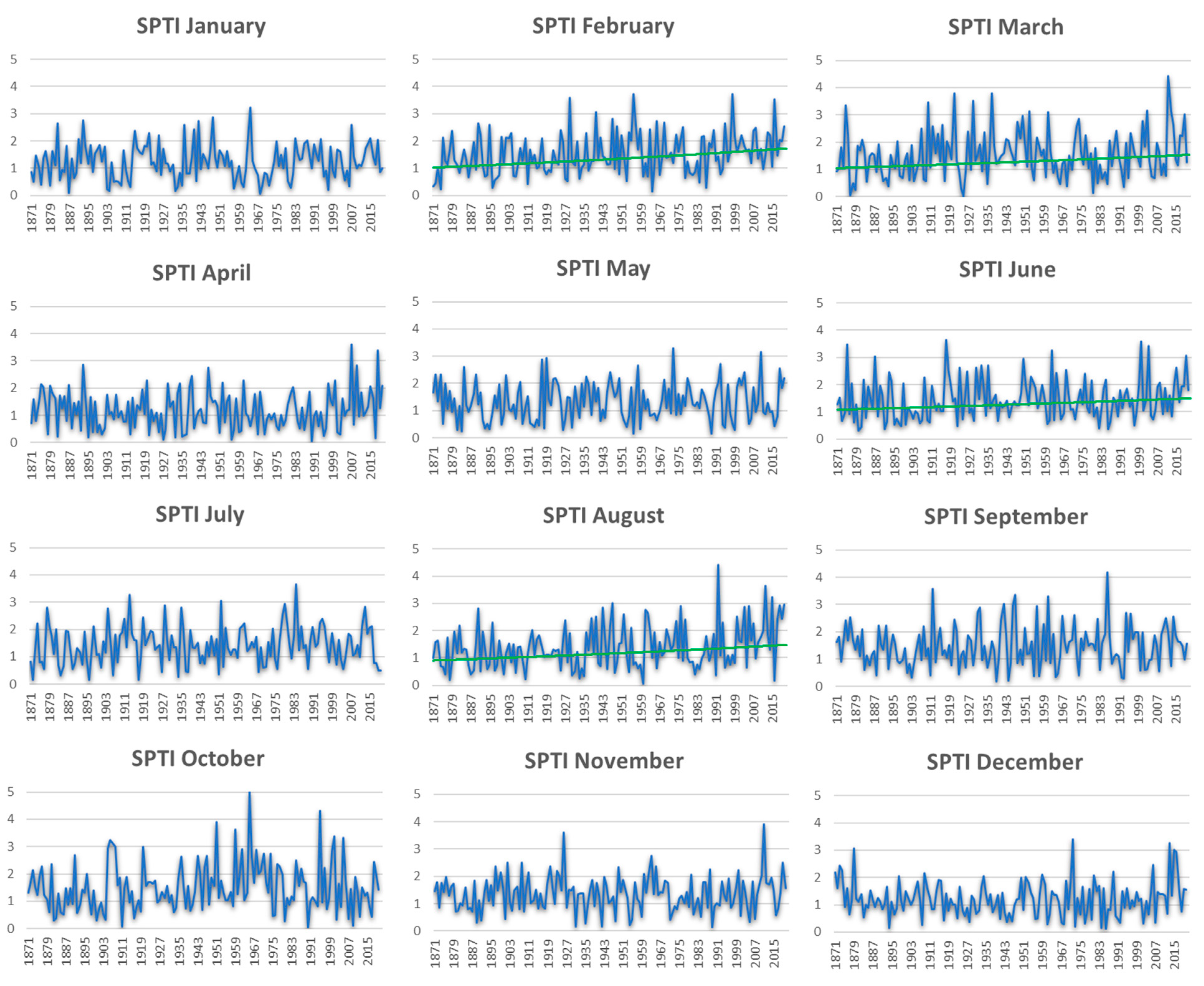
It seems surprising that while a significant change was detected in one dimension for the month of April, the null hypothesis of the same distribution for the period 1871–2020 was accepted based on the combined tests. When analysing the SPTI values, the most unusual April was in 2007, followed by the similarly dry–warm April in 2018. Above Cr1, the year 1893 remained above this dry–cool April. Figure 2 clearly shows that the highest SPTI values occurred in October.
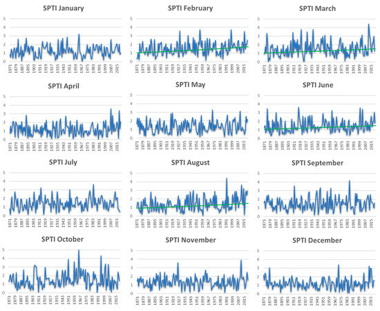
Figure 2.
SPTI values, monthly and spatial average, 1871–2020; the green line indicates the significant exponential trend.
Looking at all the months in two dimensions, the highest SPTI value belonged to the extremely dry but cool October of 1965 (Table 2). It is interesting to note that the driest October in the 150-year period was followed by the wettest November of the whole period in 1965, which was also cooler than average. Although this SPTI exceeded the critical level of mild (Cr1), it was far less unusual than the dry–cool November of 2011, which exceeded Cr2. The highest absolute value of the SPI values was also associated with the extremely dry October of 1965, while the maximum of the STI values was the hot August of 1992. Table 2 also shows that for each month, the extreme dryness was considered extreme in terms of precipitation, while for temperature, the extremes of extreme cold and extreme heat had the highest STI values in proportions of approximately 50:50. The years in the SPTI year series where one of the elements alone represents an extreme are shown in bold. For the month of August, the STI was at an absolute extreme, but the SPI was only slightly behind 2012 with a similarly dry month. In February, the 1956 precipitation and extreme cold represented the extreme value, while in unidimensional terms this year did not appear as an absolute extreme value. The same was true of July, where the dry and cool July of 1984 was the extreme. In the case of the other months, the following very dry months appeared as two-dimensional extremes with warmer than average mean temperatures: March, April, May, June, September and December, while October and November appeared as cooler.

Table 2.
Maximum SPTI values and year of maximum, maximum SPI values and year of maximum, and maximum STI values and year of maximum for all three cases: spatial average, 1871–2020. The maximum values are marked in red.
As a result of Test1, the SPTI value exceeded Cr3 in seven months, while for Test2 it exceeded Cr2 in five months. As a result of Test3, the null hypothesis could not be accepted for four months, with the largest change occurring in the extreme values in February and August. Over the whole period, the extreme value increased by 68% in February and 63% in August. In June and March, the increase was 39% and 46%, respectively, with no significant one-way change in the other months.
4.2. Analysis of Spatial SPTI Values
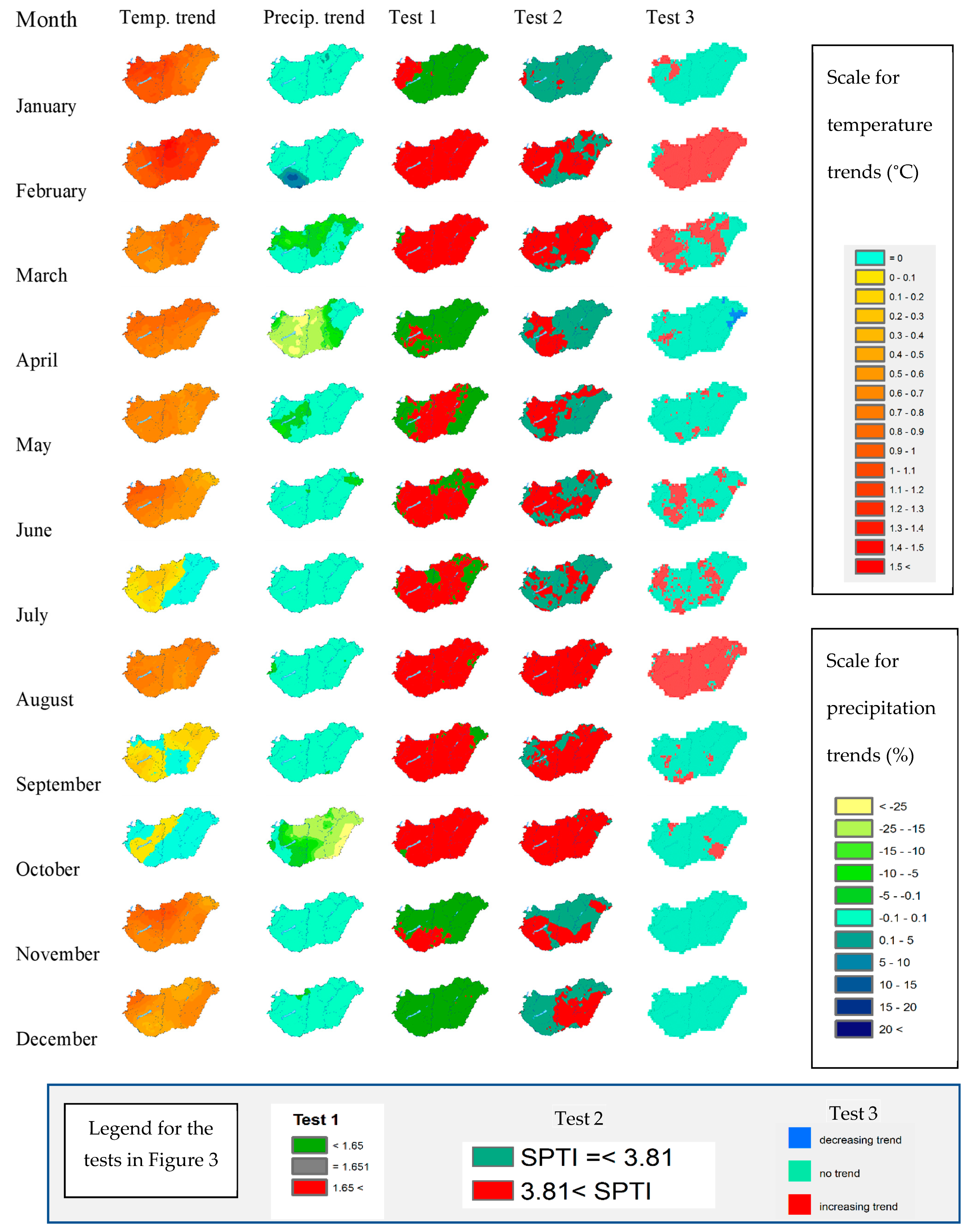
Turning our attention to the results of the spatial studies, we first noted that, as with the results presented in the spatial average, the one-dimensional trends for each month were examined and the three tests for whether there was a change over the entire period in the ensemble tests were performed. For each month, the one-dimensional trends and the results of the three statistical tests are shown in Figure 3.
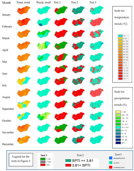
Figure 3.
Temperature and precipitation trends. Test1, Test2 and Test3 results per month for the period 1871–2020.
Results of the spatial tests
The results are shown in Figure 3, Figure 4 and Figure 5 and Figure A1, Figure A2, Figure A3, Figure A4, Figure A5, Figure A6, Figure A7, Figure A8, Figure A9, Figure A10, Figure A11, Figure A12, Figure A13, Figure A14, Figure A15, Figure A16, Figure A17, Figure A18, Figure A19, Figure A20, Figure A21 and Figure A22. The one-dimensional trends of the monthly mean temperature were similar, showing a one-way significant increase in temperature for the whole country except for the months of July, September and October (Figure 3). In these months, only a small area showed a slight increasing trend. The winter months showed the greatest warming, with February leading. Turning to the unidimensional trends in the monthly precipitation totals, February was the only month with a larger area of increasing precipitation. Although such an area in January could be found, it was very small. What was most striking was the decrease in precipitation in April and October. In the other months, no significant unidirectional change could be detected over most of the country.
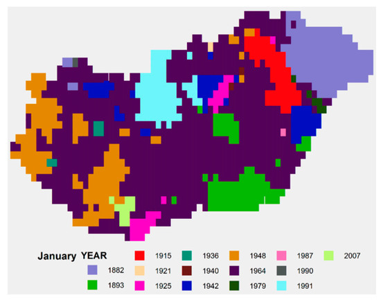
Figure 4.
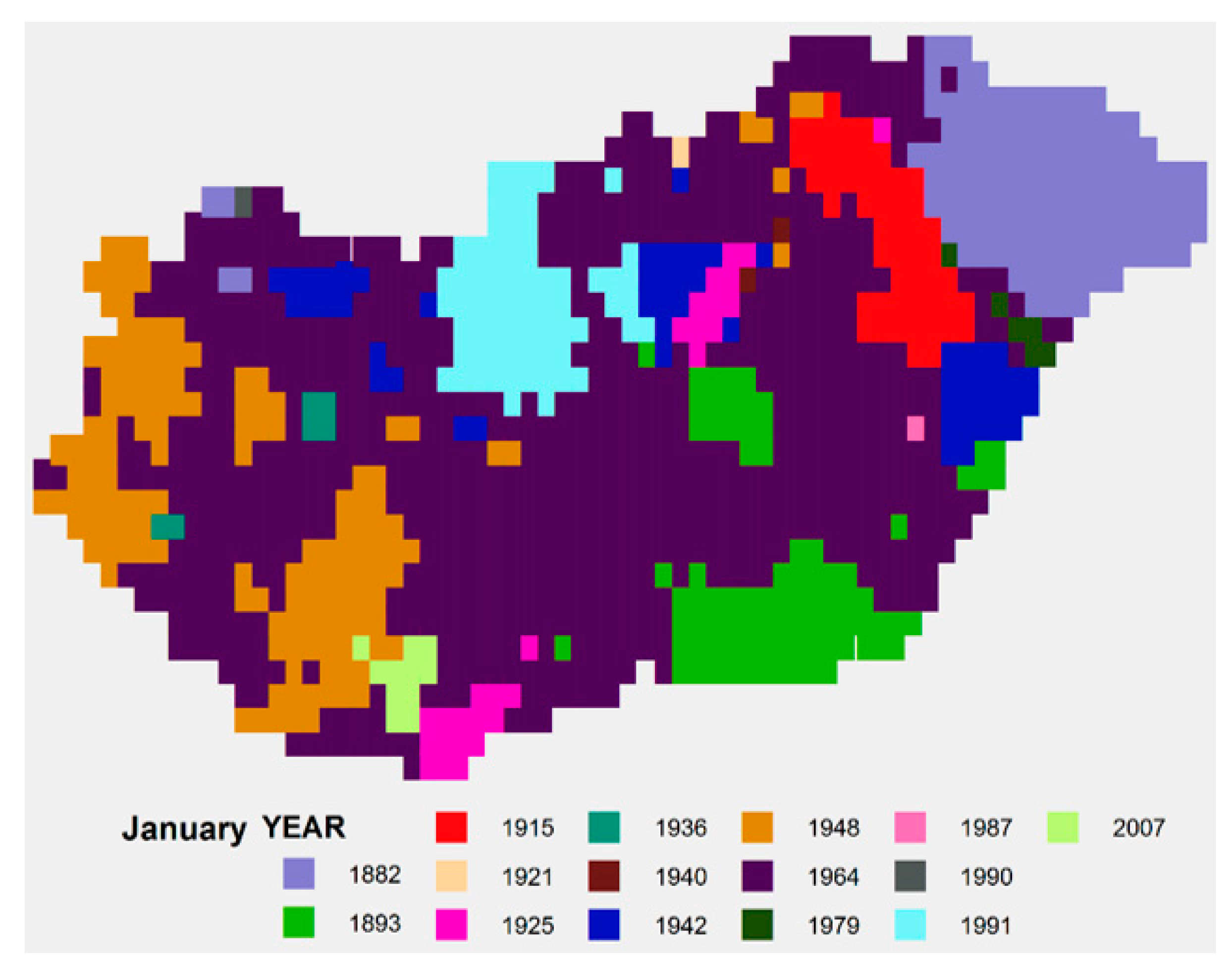
January: Year of maximum SPTI values, 1871–2020.
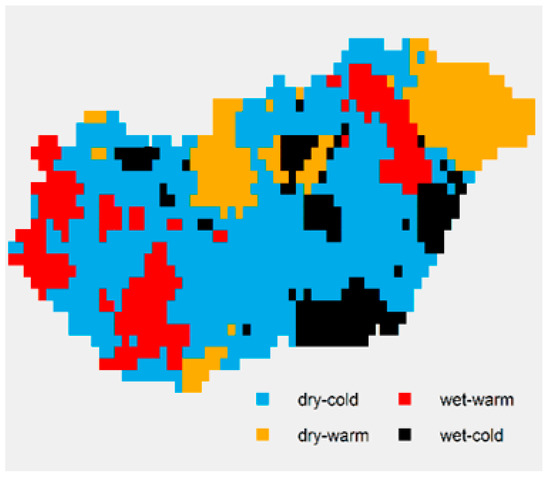
Figure 5.
Characteristics of extreme months (January).
When the results of all three tests were combined in the two-dimensional analyses, Test1 alone showed a country-wide change. The February values exceeded the critical value (Cr3) at each point in Hungary. For Test1, the areas where the test statistic (TS1) exceeded Cr3 are shown in green and those points where the values are below it are highlighted in red. The same was conducted for Test2, with red areas showing SPTI values exceeding Cr2 and green areas showing those not exceeding it. The Test3 results are coloured green where there was no significant trend. Areas where the SPTI values displayed a significant increase are marked in red and areas where they displayed a decrease are marked in blue. In only one case was there a significant decrease in extremes, i.e., in April in the eastern part of the country, while in this month there was a significant increase in the central part of the western part of the country (mainly around Lake Balaton).
For the maximum SPTI values, the year in which the extreme month occurred was sought. This gave an idea of which month may be considered extreme and whether it occurred recently or early in the period. It is important to note that in all cases the calibration period was the 1871-1900 climate normal. In the following section, only the month of January is shown, and the analysis of the other months and their graphs are presented in the Appendix A.
January: Only in the western half of the country was climate change evident over a larger area, which was again more likely to be captured by the first test (Figure 3). Figure 4 and Figure 5 show that the dry–cool January of 1964 was the extreme for most of the country. However, in the eastern part of the country, a dry–warm (1882) and wet–cold (1893) January was considered extreme. Over a larger area, dry–hot (1991) and wet–hot (1915, 1948) Januarys were also extreme. The extremely cool January of 1942 also appeared scattered across the country; this was an extreme January in terms of temperature and had above average precipitation.
5. Conclusions
The norm method based on the probability distribution of the elements and its application to monthly precipitation sum and mean temperature time series was presented here. The SPTI values for each month were determined and the monthly extremes defined. First, the spatial mean values were examined. Comparing the SPTI values for the 12 months of all years, the highest absolute value was for October 1965. So, the most unusual month in the entire 150 years when looking at these two dimensions was a very dry, warm October. In second place was another dry, hot month, i.e., March 2012, while August 1992 was in third place. In the latter case, yet another hot and dry month also represented an extreme. Interestingly, the maximum absolute SPI values were all associated with a dry month, albeit in different seasons. If, in the case of temperature, September 1912 and July 1913 are ignored, extreme cold was considered unusual from December to March, and extreme heat was considered unusual from April to November, based on a comparison of STI values. In 1912–13, cold and wet periods across Europe were recorded, which were clearly attributable to the Alaskan volcanic eruption [45,46]. However, if this value is ignored, the higher absolute STI values in September could be associated with warmer months, but in July the cold month remained the extreme. Looking at the results of Test1, the SPTI value exceeded Cr3 in seven months, while for Test2 it exceeded Cr2 in five months’ SPTI values. Turning to the results of Test3, the null hypothesis could not be accepted for four months, with the largest change occurring in the extreme values in February and August. Over the whole period, the extreme value increased by 68% in February and 63% in August. In June and March, the increase was 39% and 46%, respectively, with no significant one-way change in the other months.
Based on the spatial analysis, Test1 indicated climate change over most of the country in two dimensions for the months of February, March and May to October. Test2 also detected a change over most of the country, but this test also indicated climate change in two dimensions for the month of December for the whole of the Great Plain. For the month of November, Test2 also indicated a change over a larger area than Test1. A significant change in SPTI values was detected by Test3, which indicated a change for the whole of Hungary for the months of February and August but no change at any point for the months of November and December. For the other months, Test3 showed only small areas of change. There was only one case where the extremes decreased, namely, in April in the eastern part of the country.
The spatial analysis showed that the dry–warm months could generally be considered extreme over the greatest area. This was true for March, April, May, August, September and December. Dry–cold extremes occurred over the most extensive areas in January, July and November. The only month where wet–cold was most unusual was February. Wet–warm extremes occurred over a smaller area in most months, but not nearly as much as dry–warm months.
It is worth noting that the method presented here may, of course, be applied to other meteorological elements and even to derived values. These could be various extreme indices to characterise the climate of the Carpathian Basin and its changes more precisely.
Author Contributions
Conceptualization, B.I. and T.S.; methodology, T.S.; software, T.S. and B.I.; validation, B.I.; investigation, B.I; writing—original draft preparation, B.I. and T.S.; visualization, B.I.; supervision, M.L. and R.P.; writing—review and editing, M.L. and R.P. All authors have read and agreed to the published version of the manuscript.
Funding
This research received no external funding.
Institutional Review Board Statement
Not applicable.
Informed Consent Statement
Not applicable.
Data Availability Statement
Not applicable here.
Conflicts of Interest
The authors declare no conflict of interest.
Appendix A

Figure A1.
February: Year of maximum SPTI values, 1871–2020.
Figure A1.
February: Year of maximum SPTI values, 1871–2020.
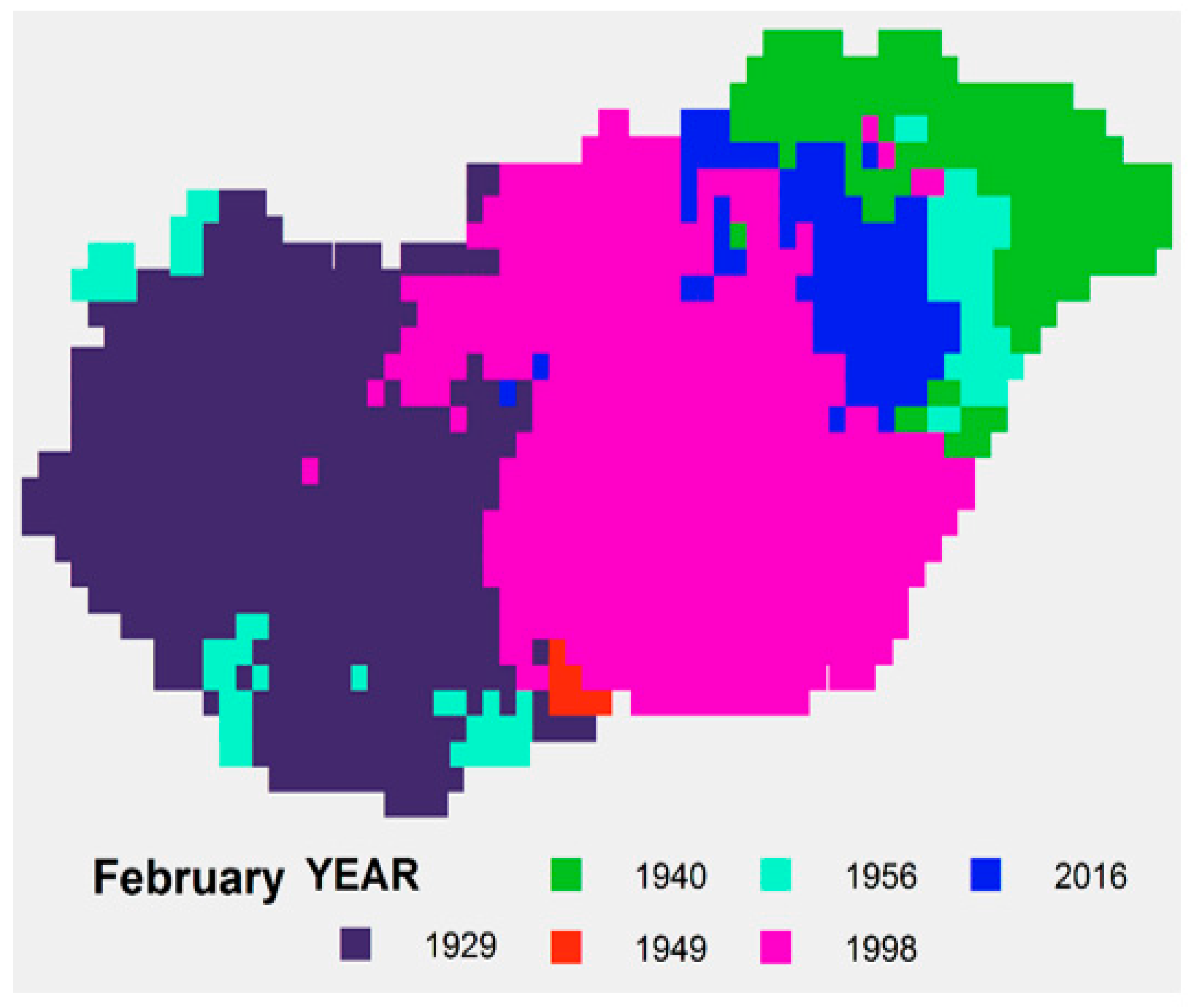

Figure A2.
Characteristics of extreme months (February).
Figure A2.
Characteristics of extreme months (February).
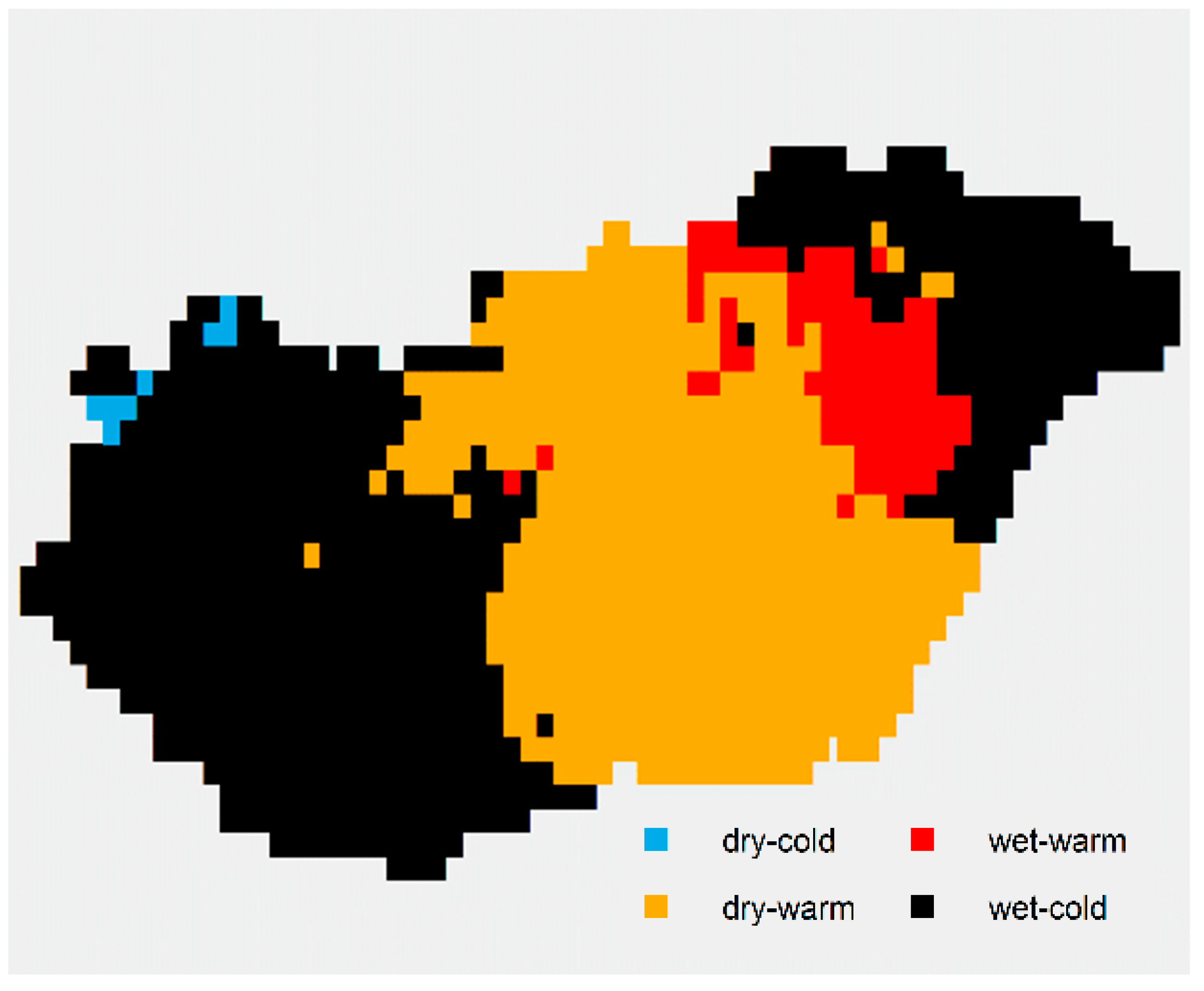
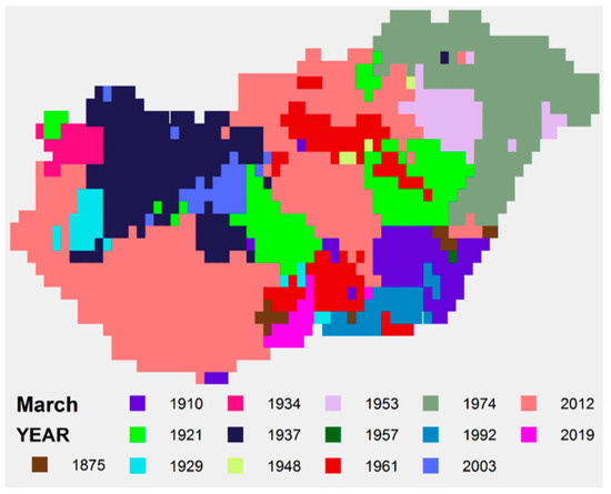
Figure A3.
March: Year of maximum SPTI values, 1871–2020.
Figure A3.
March: Year of maximum SPTI values, 1871–2020.


Figure A4.
Characteristics of extreme months (March).
Figure A4.
Characteristics of extreme months (March).
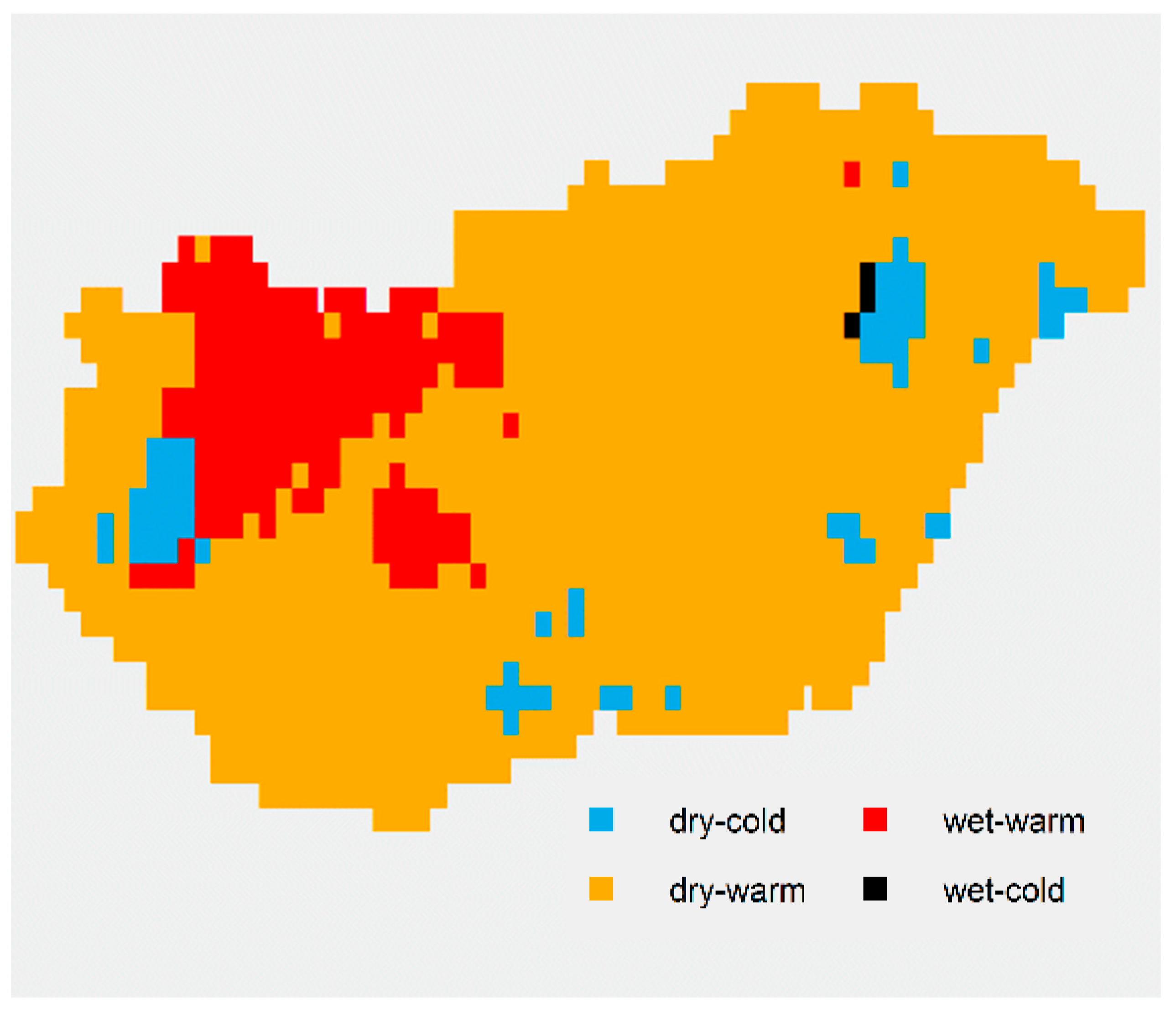
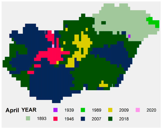
Figure A5.
April: Year of maximum SPTI values, 1871–2020.
Figure A5.
April: Year of maximum SPTI values, 1871–2020.
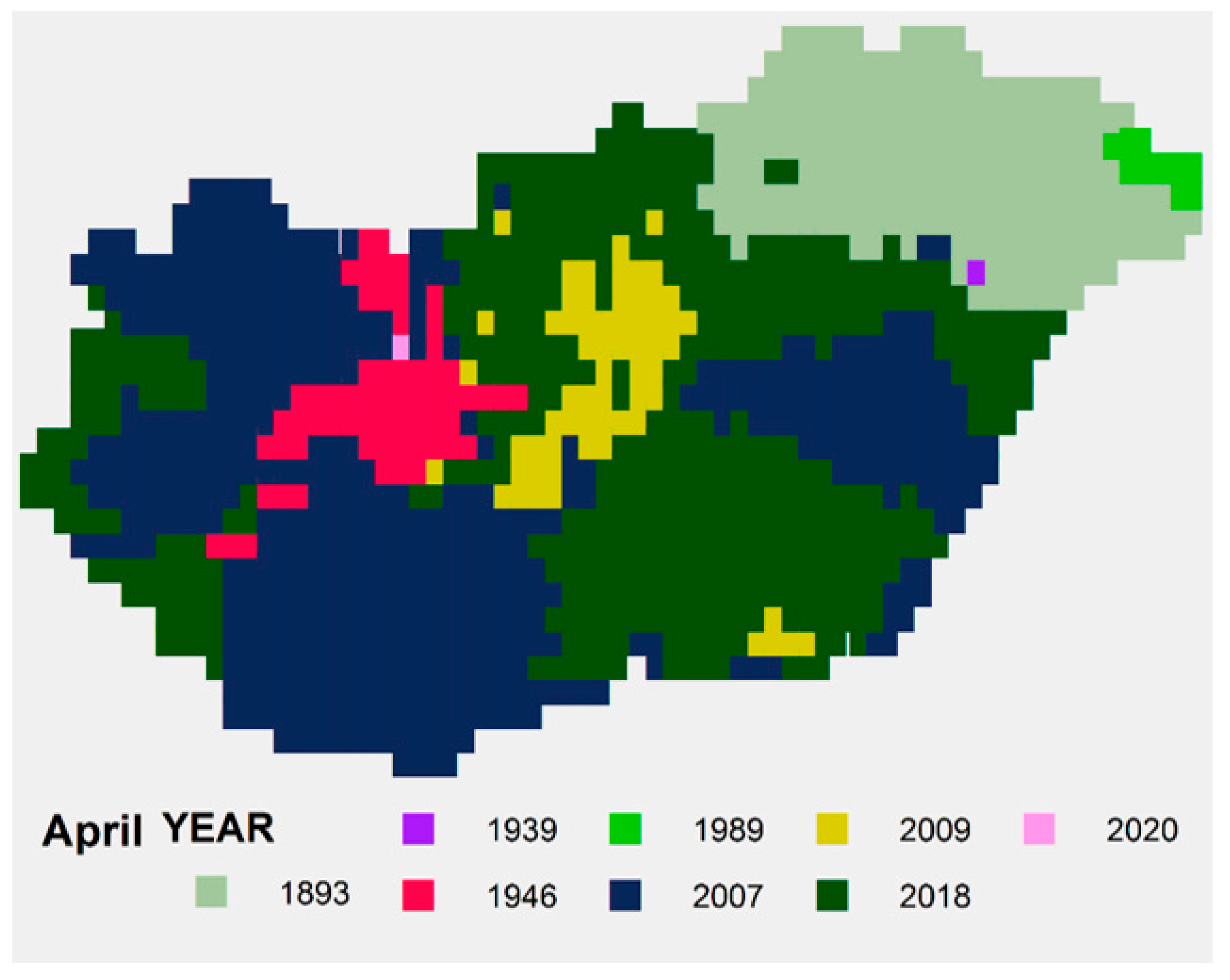

Figure A6.
Characteristics of extreme months (April).
Figure A6.
Characteristics of extreme months (April).
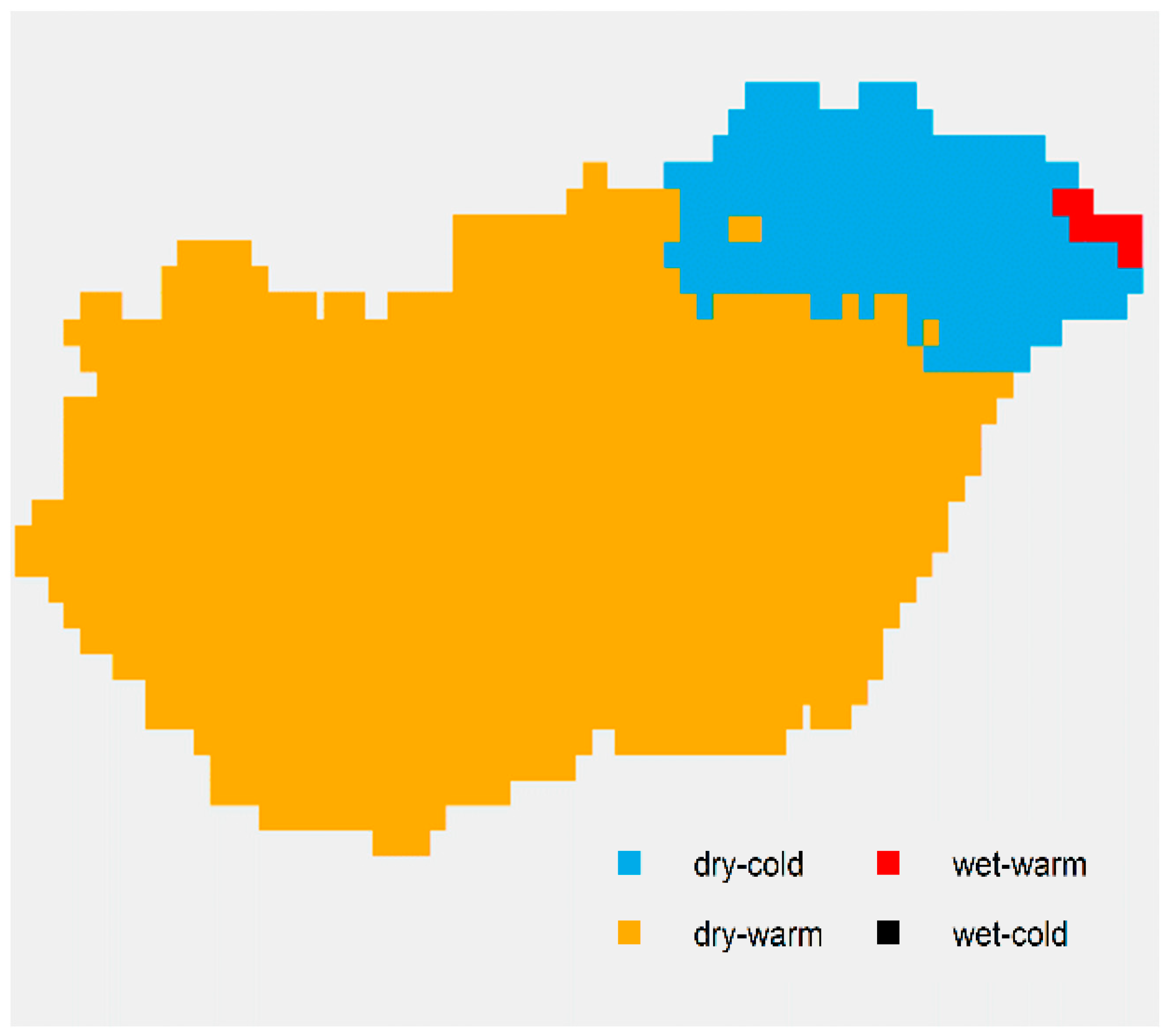

Figure A7.
May: Year of maximum SPTI values, 1871–2020.
Figure A7.
May: Year of maximum SPTI values, 1871–2020.
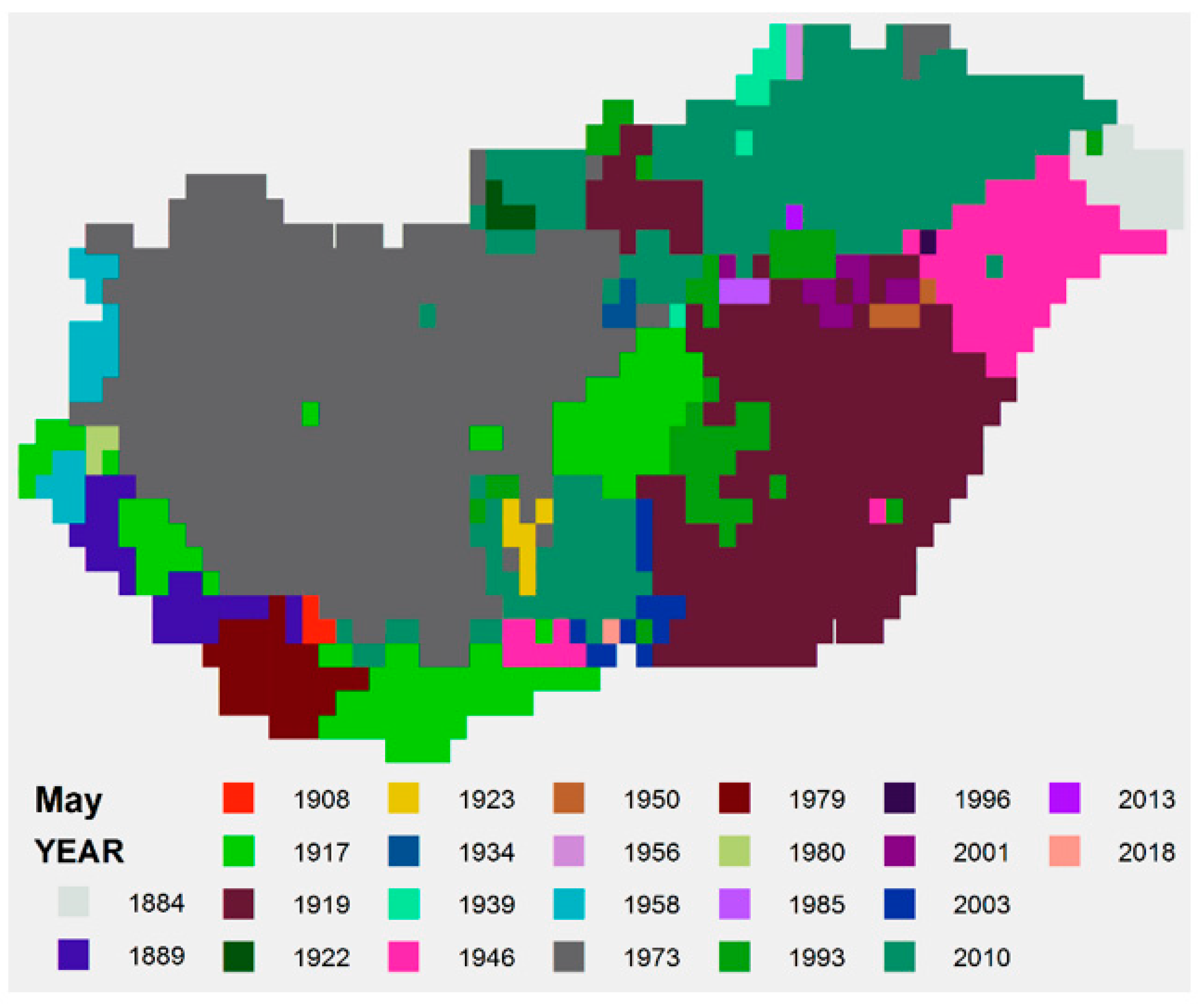
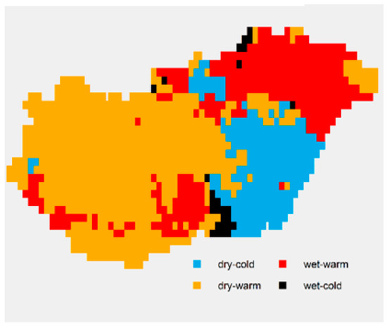
Figure A8.
Characteristics of extreme months (May).
Figure A8.
Characteristics of extreme months (May).


Figure A9.
June: Year of maximum SPTI values, 1871–2020.
Figure A9.
June: Year of maximum SPTI values, 1871–2020.
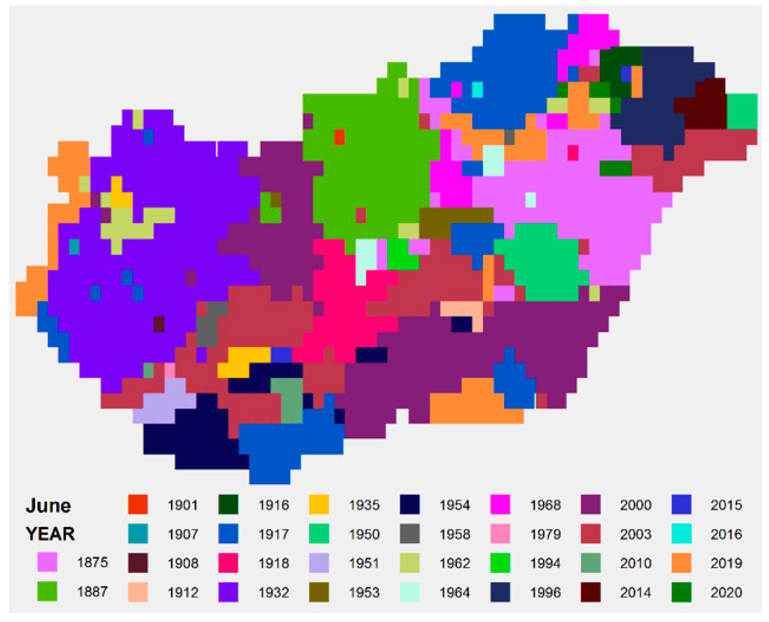
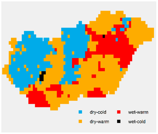
Figure A10.
Characteristics of extreme months (June).
Figure A10.
Characteristics of extreme months (June).

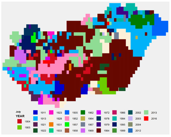
Figure A11.
July: Year of maximum SPTI values, 1871–2020.
Figure A11.
July: Year of maximum SPTI values, 1871–2020.

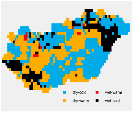
Figure A12.
Characteristics of extreme months (July).
Figure A12.
Characteristics of extreme months (July).

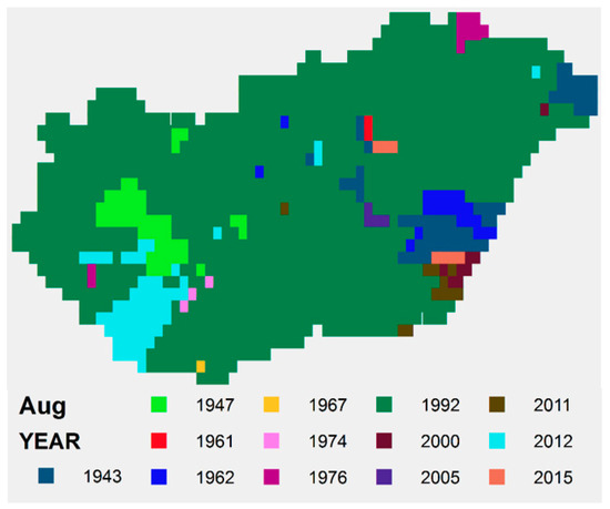
Figure A13.
August: Year of maximum SPTI values, 1871–2020.
Figure A13.
August: Year of maximum SPTI values, 1871–2020.
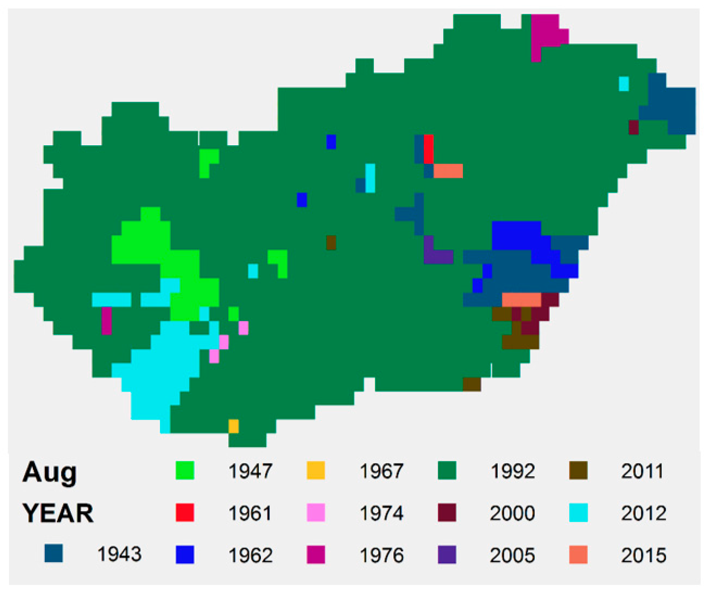

Figure A14.
Characteristics of extreme months (August).
Figure A14.
Characteristics of extreme months (August).
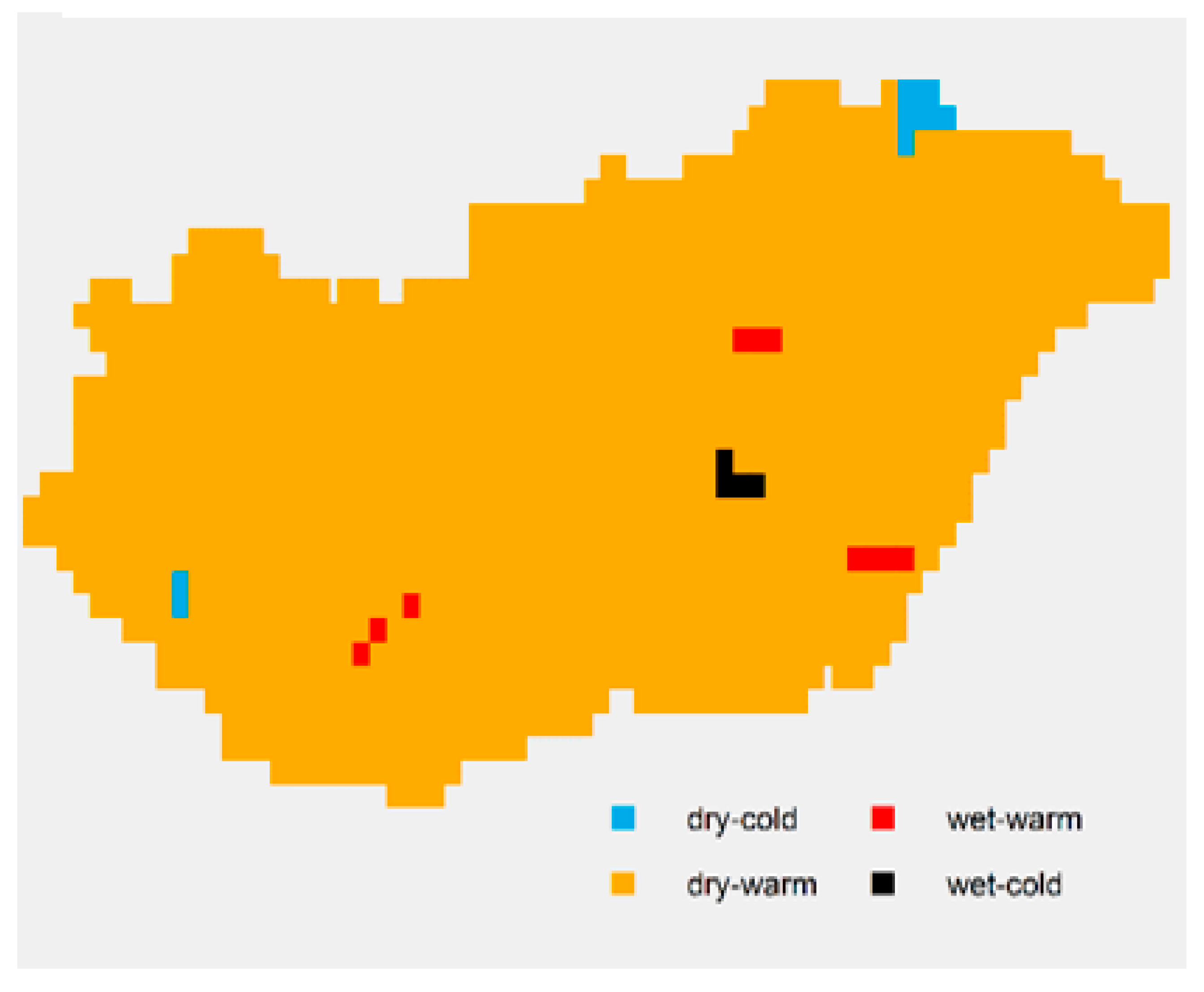
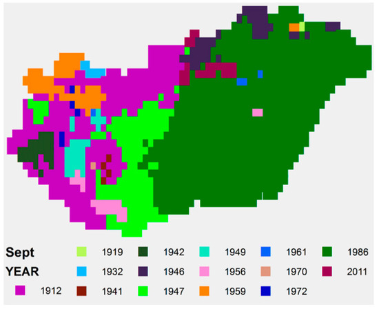
Figure A15.
September: Year of maximum SPTI values, 1871–2020.
Figure A15.
September: Year of maximum SPTI values, 1871–2020.
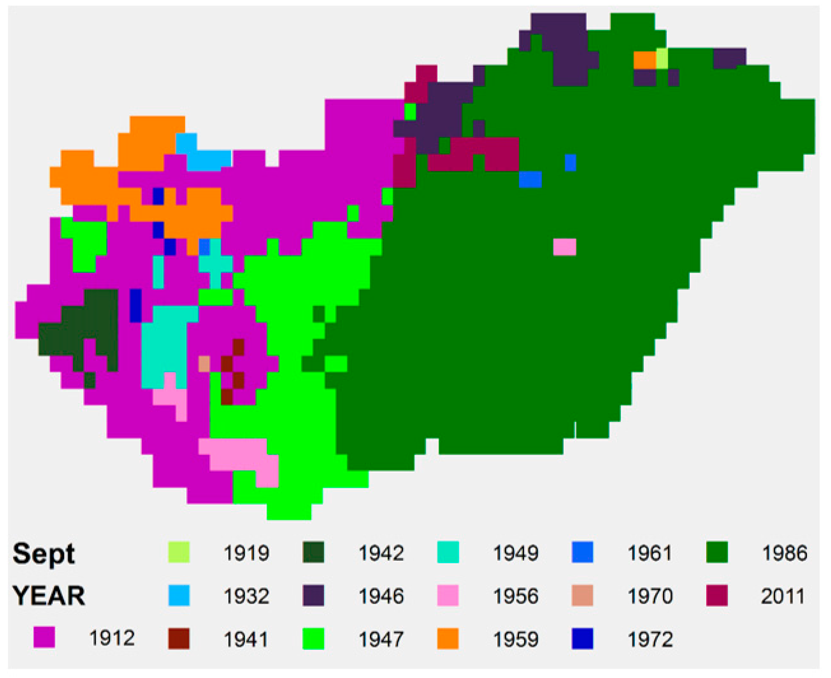
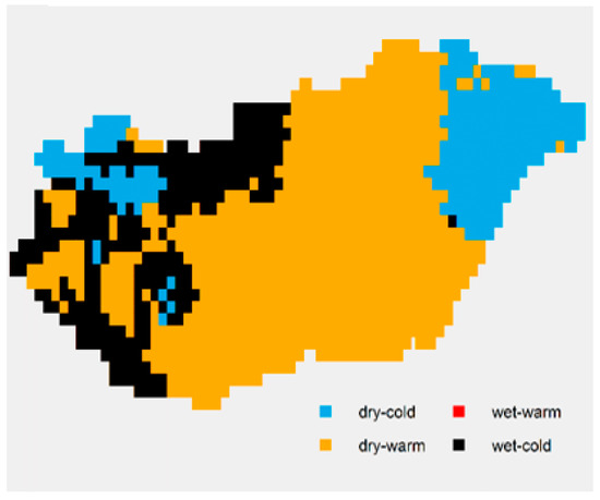
Figure A16.
Characteristics of extreme months (September).
Figure A16.
Characteristics of extreme months (September).

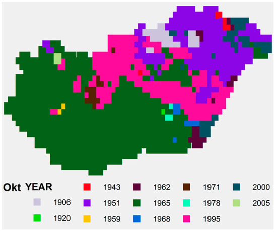
Figure A17.
October: Year of maximum SPTI values, 1871–2020.
Figure A17.
October: Year of maximum SPTI values, 1871–2020.
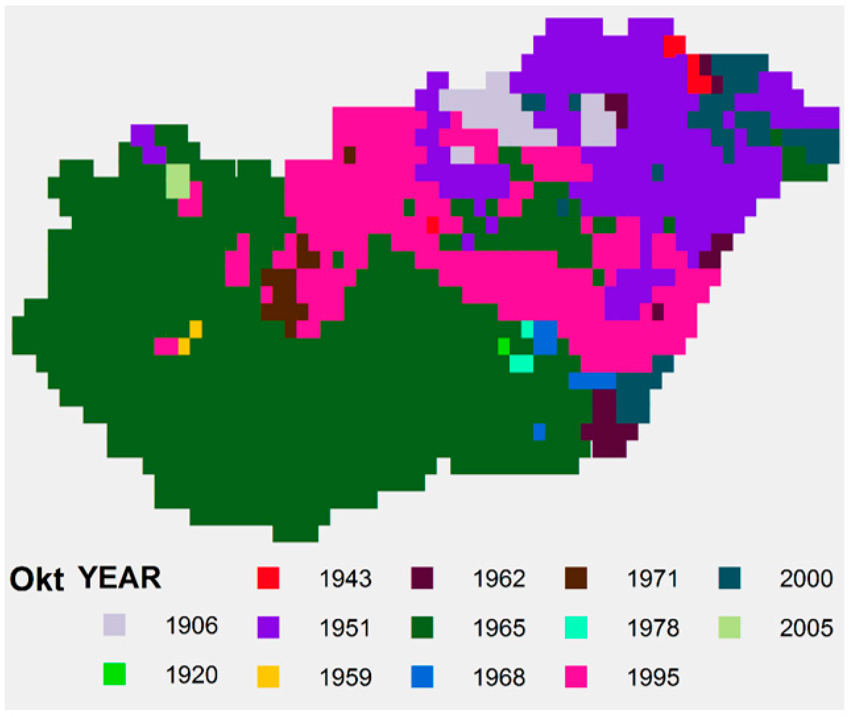
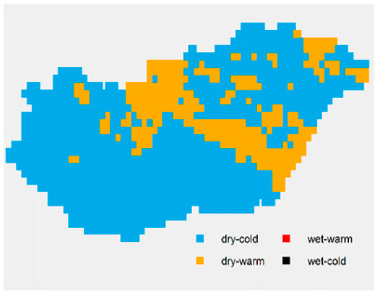
Figure A18.
Characteristics of extreme months (October).
Figure A18.
Characteristics of extreme months (October).

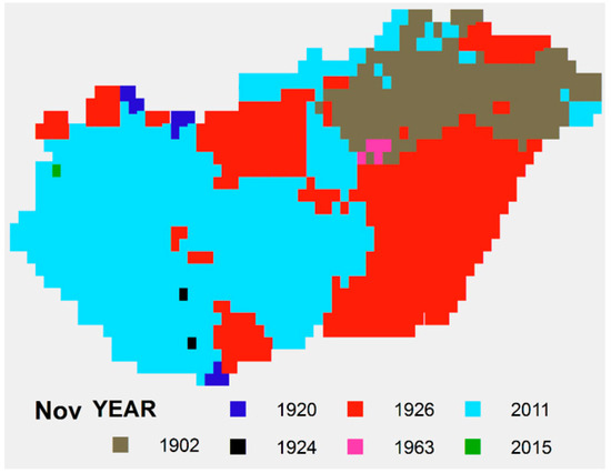
Figure A19.
November: Year of maximum SPTI values, 1871–2020.
Figure A19.
November: Year of maximum SPTI values, 1871–2020.
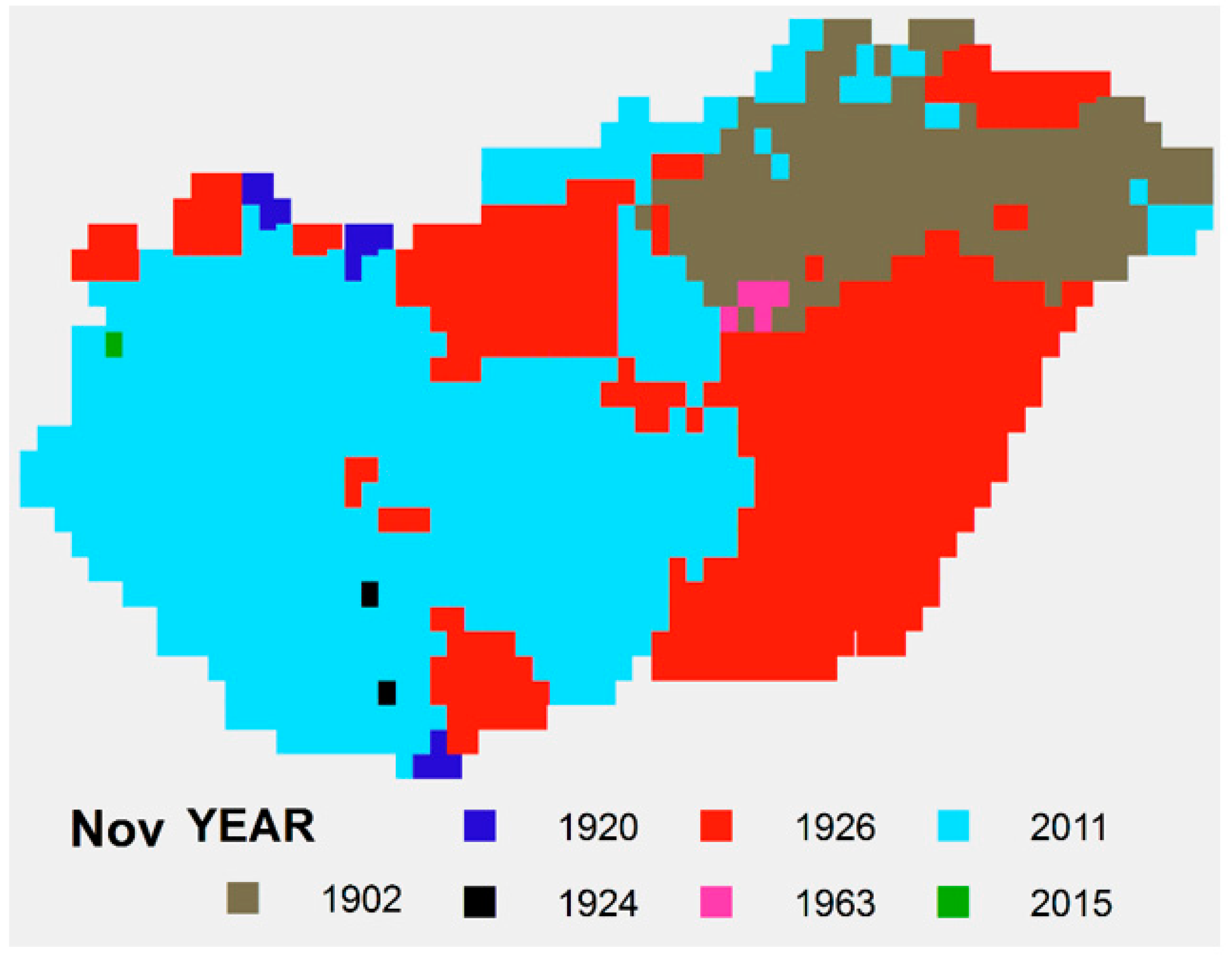
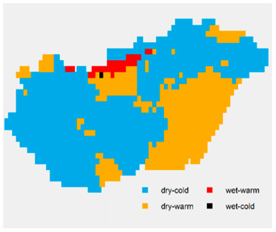
Figure A20.
Characteristics of extreme months (November).
Figure A20.
Characteristics of extreme months (November).
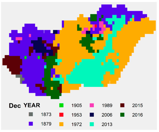
Figure A21.
December: Year of maximum SPTI values, 1871–2020.
Figure A21.
December: Year of maximum SPTI values, 1871–2020.


Figure A22.
Characteristics of extreme months (December).
Figure A22.
Characteristics of extreme months (December).
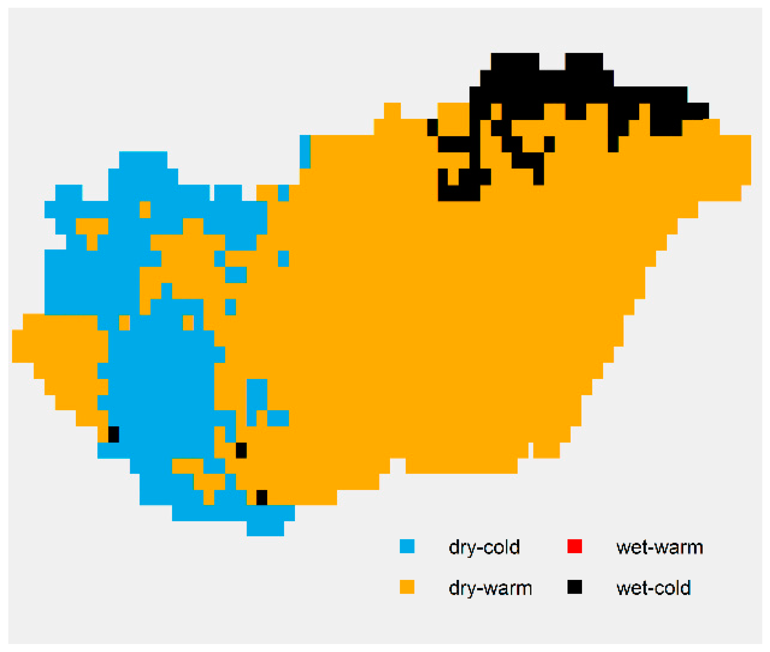
February: All three tests indicated a change over most of the country, and when combined, the results showed that the climate was changing over the whole country, if precipitation and temperature were examined together. (Figure 3). In the Transdanubian region and the eastern part of the country (Figure A1 and Figure A2), a wet–cool February was unusual (1929, 1940 and 1956). In the central part of the country, a very dry–hot February was considered extreme (1949 and 1998), but a large area coverage was unusual for the wet–hot February of 2016.
March: Test1 showed the largest area of change, and if the three maps are compared, it is possible to say that only at the eastern tip of the country was there a small area where change was not detectable (Figure 3). Looking at Figure A3 and Figure A4, the picture is variegated, however, with the exception of two extreme years, an extreme March was very dry and hot. One of these exceptions was the dry–cold March of 1875, which occurred in small areas, and the other was the wet–hot March of 1937 in and around the plains in north-western Hungary (Kisalföld).
April: A large part of the Transdanubian region showed a change. Only a small area of the Danube–Tisza interfluve and the region beyond the Tisza River to the east showed a change in climate based on the combined analysis of the two elements, while the Alpine foreland (Alpokalja) showed no change (Figure 3). Figure A5 and Figure A6 shows that only in the easternmost part of the country did the hot–wet April of 1989 count as extreme, and that in the north-eastern part of the country a large area was affected by the dry–cold character of that month in 1893. In all other places, a dry–hot April was the most unusual, and it should be noted that almost all instances of this fell within the last two decades (2007, 2009, 2018 and 2020).
May: The degree of variation was similar to that described for April, with the difference that a large area of change was also detectable in the Northern Mountains (Északi-középhegység) and the Danube–Tisza interfluve (Figure 3). In Figure A7 and Figure A8, the largest area was the dry, warm May of 1973, but most of the years listed were also associated with a dry–warm May. The exceptions were the years with a wet–hot May that dominated the northern and eastern parts of the country, and these were seen in the years 1946, 1996, 2010 and 2013. There were also extreme wet–cold May years, namely 1939 and 1956. There were also scattered extreme very dry–cool years, namely 1919 and 1980.
June: When the three tests were evaluated together, only the Northern Mountains and the Kőrösök region showed no climate change (Figure 3). The Junes of 1908, 1917, 1994, 1996, 2000, 2015 and 2019 had in common that they were very dry–hot months. Thus, a dry–hot June was considered extreme in most of Hungary. The map also shows dry–cold extremes over large areas in 1887, 1918 and 1932. A wet–warm June (1875, 1964 and 2010) and a single small area in Transdanubia with a wet–cold one (1958) were also considered extreme (Figure A9 and Figure A10).
July: There was change over most of the country, with small areas around Budapest and the western and eastern extremities of the country, where change was not detectable (Figure 3). The most varied picture is shown in Figure A11 and Figure A12. It was almost impossible to analyse every point. It was clear that the most unusual case was the dry–cool July of 1984, but in the other areas such a month would also appear as an extreme case, for example in 1922, 1933, 1935, 1952, 1964, 1969, 1979, 1984, 1986, 1995 and 2004. Dry–hot extremes in the south were seen in 1904, 1905 and 1911, and a wet–cold July was seen in 1913, 1962 and 1978. The rainy–hot extreme years were 1957, 1972, 1999, 2002, 2003 and 2016.
August: The change was evident throughout the country (Figure 3). Figure A13 and Figure A14 show the fairly extensive area of the record hot and dry August of 1992, but most of the other years were also typical. In the north-eastern corner of the country, the dry–cool month of 1976 dominated, while a wet–warm August (1974 and 2015) could only be detected at a few points in Hungary. In any case, the already extreme wet–cool year (2005) was more extreme in the centre of the lowlands.
September: While Test3 did not show much change at many points, the other two tests showed change across almost the whole country (Figure 3). In Figure A15 and Figure A16, the first extreme September that appeared was 1986, which was also extreme on average for the country, with two-thirds of the country showing extreme results. The coldest September was 1912, which was also a wet September, and this was unusual for large areas of the Transdanubian region. Among the dry–cool Septembers were those of 1941, 1949, 1970 and 1972 in the north-western and central parts of the Transdanubian region.
October: As was the case for September, there was climate change at all points (Figure 3). The October extremes graph (Figure A17 and Figure A18) is divided between dry–warm and dry–cool years. The largest area extent was seen in the record dry and cool October of 1965, but this type was also found in 1920, 1951, 1959, 1965, 1971 and 1978. The Octobers of 1906, 1943, 1962, 1968, 1995, 2000 and 2005 were recorded as dry–hot, with these occurring more as extremes in the central part of the country
November: Change was evident over a third of the country, mainly in the south-southwest, but also along the eastern edge of the country, according to Test2 (Figure 3). As in October, only the dry–cold and dry–warm months appeared as extremes in the case of November. Over the largest area, the record dry and cooler than average November of 2011 appeared as an extreme, but so did the years 1902, 1920 and 1922. Of the dry, warm years, 1926 appeared across the largest area, but 1963 and 2015 were similar. (Figure A19 and Figure A20)
December: Test1 and Test3 showed no change, while for the entire lowland area, Test2 could be used to show two-dimensional climate change (Figure 3). Of the years in Figure A21 and Figure A22, only December 1879 could be considered a dry–cold month, with December in all the other years being dry–warm. The record dry December of 1972 was the highest two-dimensional norm, but it also proved to be the driest December in one dimension. In terms of temperature, the record cold of 1879 was the most unusual, with a large area of this year appearing in Figure A21.
References
- Jenkinson, A.F. The frequency distribution of the annual maximum (or minimum) values of meteorological events. Quart. J. Roy. Meteorol. Soc. 1955, 81, 158–172. [Google Scholar] [CrossRef]
- Naveau, P.; Hannart, A.; Ribes, A. Statistical Methods for Extreme Event Attribution in Climate Science. Ann. Rev. Stat. Appl. 2020, 7, 1–22. [Google Scholar] [CrossRef]
- de Oliveira, J.T. Extreme values and meteorology. Theor. Appl. Climatol. 1986, 37, 184–193. [Google Scholar] [CrossRef]
- Dutfoy, A.; Parey, S.; Roche, N. Multivariate Extreme Value Theory—A Tutorial with Applications to Hydrology and Meteorology. Depend. Model. 2014, 2, 30–48. [Google Scholar] [CrossRef]
- Hoogewind, K.A.; Baldwin, M.E.; Trapp, R.J. The Impact of Climate Change on Hazardous Convective Weather in the United States: Insight from High-Resolution Dynamical Downscaling. J. Climate 2017, 30, 10081–10100. [Google Scholar] [CrossRef]
- Demski, C.; Capstick, S.; Pidgeon, N.; Sposato, R.G.; Spence, A. Experience of extreme weather affects climate change mitigation and adaptation responses. Clim. Chang. 2017, 140, 149–164. [Google Scholar] [CrossRef]
- Carter, D.J.T.; Challeron, P.G. Estimating return values of environmental parameters. Quart. J. Roy. Meteorol. Soc. 1981, 107, 259–266. [Google Scholar] [CrossRef]
- Lakatos, M.; Izsák, B.; Szentes, O.; Hoffmann, L.; Kircsi, A.; Bihari, Z. Return values of 60-minute extreme rainfall for Hungary. Időjárás 2020, 124, 143–156. [Google Scholar] [CrossRef]
- Klein Tank, A.M.G.; Zwiers, F.W.; Zhang, X. Guidelines on Analysis of Extremes in a Changing Climate in Support of Informed Decisions for Adaptation; World Meteorological Organization: Geneva, Switzerland, 2009; Climate data and monitoring WCDMP-No. 72; WMO-TD No. 1500. [Google Scholar]
- Szentimrey, T. Többdimenziós Éghajlati Idősorok “Extrémumainak” Vizsgálata. (Examination of "Extremes" in Multidimensional Climate Time Series); Meteorológiai Tudományos Napok’99 Kiadványa: Budapest, Hungary, 1999; pp. 77–88. (In Hungarian) [Google Scholar]
- Matyasovszky, I. Extreme temperature and precipitation years in Hungary during last century. Időjárás 2001, 105, 157–164. [Google Scholar]
- Szentimrey, T.; Izsák, B. Joint examination of climate time series based on a statistical definition of multidimensional extreme. Időjárás 2022, 126, 159–184. [Google Scholar] [CrossRef]
- Kiriliouk, A.; Naveau, P. Climate extreme event attribution using multivariate peaks-over-thresholds modeling and counterfactual theory. Ann. Appl. Stat. 2020, 14, 1342–1358. [Google Scholar] [CrossRef]
- Cooley, D.; Thibaud, E. Decompositions of dependence for high-dimensional extremes. Biometrika 2019, 106, 587–604. [Google Scholar] [CrossRef]
- Trenberth, K.; Shea, D. Relationship between precipitation and surface temperature. Geophys. Res. Lett. 2005, 32, L14703. [Google Scholar] [CrossRef]
- Zhao, W.; Khalil, M.A.K. The Relationship between Precipitation and Temperature over the Contiguous United States. J. Climate 1993, 6, 1232–1236. [Google Scholar] [CrossRef]
- Parzen, E. On the estimation of probability density function and mode. Ann. Math. Stat. 1962, 33, 1065–1076. [Google Scholar] [CrossRef]
- Rosenblatt, M. On some nonparametric estimates of a density function. Ann. Math. Stat. 1956, 27, 832–837. [Google Scholar] [CrossRef]
- Lakatos, M.; Matyasovszky, I. Analysis of the extremity of precipitation intensity using the POT method. Időjárás 2004, 108, 163–171. [Google Scholar]
- de Oliviera, J.T. Bivariate Models for Extremes. In Statistical Extremes and Applications; Reidel: Dortrecht, Holland, 1984; pp. 131–153. [Google Scholar]
- Wazneh, H.; Arain, M.; Coulibaly, P.; Gachon, P. Evaluating the Dependence between Temperature and Precipitation to Better Estimate the Risks of Concurrent Extreme Weather Events. Adv. Meteorol. 2020, 2020, 8763631. [Google Scholar] [CrossRef]
- Zhao, N.; Lin, W.T. A copula entropy approach to correlation measurement at the country level. Appl. Math. Comput. 2011, 218, 628–642. [Google Scholar] [CrossRef]
- Ohlwein, C.; Friederichs, P. Multivariate non-normally distributed random variables in climate research—Introduction to the copula approach. Nonlinear Proc. Geophys. 2008, 15, 761–772. [Google Scholar]
- Renard, B.; Lang, M. Use of a Gaussian copula for multivariate extreme value analysis: Some case studies in hydrology. Adv. Water Resour. 2007, 30, 897–912. [Google Scholar] [CrossRef]
- Yan, J. Enjoy the Joy of Copulas: With a Package copula. J. Stat. Software 2007, 21, 1–21. [Google Scholar] [CrossRef]
- Gudendorf, G.; Segers, J. Extreme-Value Copulas. Lecture Notes in Statistics. LNSP 2010, 198, 127–145. [Google Scholar]
- Wang, J.; Rong, G.; Li, K.; Zhang, J. Analysis of Drought Characteristics in Northern Shaanxi Based on Copula Function. Water 2021, 13, 1445. [Google Scholar] [CrossRef]
- Ferreira, A.; de Haan, L. On the block maxima method in extreme value theory: PWM estimators. Ann. Statist. 2015, 43, 276–298. [Google Scholar] [CrossRef]
- Izsák, B.; Szentimrey, T. To what extent does the detection of climate change in Hungary depend on the choice of statistical methods? GEM—Int. J. Geomath. 2020, 11, 17. [Google Scholar] [CrossRef]
- Szentimrey, T. Manual of Homogenization Software MASHv3.03; Hungarian Meteorological Service: Budapest, Hungary, 2014. [Google Scholar]
- Szentimrey, T.; Bihari, Z.; Lakatos, M. Quality control procedures in MISH-MASH systems, 10th EMS Annual Meeting. In Proceedings of the 10th European Conference on Applications of Meteorology (ECAM) Abstracts, Zürich, Switzerland, 13–17 September 2010. [Google Scholar]
- Szentimrey, T. Theoretical questions of daily data homogenization. Időjárás 2013, 117, 113–122. [Google Scholar]
- Cressie, N. Statistics for Spatial Data; Wiley: New York, NY, USA, 1991. [Google Scholar]
- Szentimrey, T.; Bihari, Z. Manual of Interpolation Software MISHv1.03; Hungarian Meteorological Service: Budapest, Hungary, 2014; p. 89. [Google Scholar]
- Szentimrey, T.; Bihari, Z.; Lakatos, M.; Szalai, S. Mathematical, methodological questions concerning the spatial interpolation of climate elements. Időjárás 2011, 115, 1–11. [Google Scholar]
- Lakatos, M.; Szentimrey, T.; Bihari, Z.; Szalai, S. Creation of a homogenized climate database for the Carpathian region by applying the MASH procedure and the preliminary analysis of the data. Időjárás 2013, 117, 143–158. [Google Scholar]
- Spinoni, J.; Szalai, S.; Szentimrey, T.; Lakatos, M.; Bihari, Z.; Nagy, A.; Németh, Á.; Kovács, T.; Mihic, D.; Dacic, M.; et al. Climate of the Carpathian Region in the period 1961–2010: Climatologies and trends of 10 variables. Int. J. Climatol. 2015, 35, 1322–1341. [Google Scholar] [CrossRef]
- Venema, V.; Mestre, O.; Aguilar, E.; Auer, I.; Guijarro, J.A.; Domonkos, P.; Vertacnik, G.; Szentimrey, T.; Štěpánek, P.; Zahradnicek, P.; et al. Benchmarking monthly homogenization algorithms. Clim. Past. 2012, 8, 89–115. [Google Scholar] [CrossRef]
- Gutowski, W.J., Jr.; Ullrich, P.A.; Hall, A.; Leung, L.R.; O’Brien, T.A.; Patricola, C.M.; Arritt, R.W.; Bukovsky, M.S.; Calvin, K.V.; Feng, Z.; et al. The Ongoing Need for High-Resolution Regional Climate Models: Process Understanding and Stakeholder Information. Bull. Am. Meteorol. Soc. 2020, 101, E664–E683. [Google Scholar] [CrossRef]
- Bandhauer, M.; Isotta, F.; Lakatos, M.; Lussana, C.; Båserud, L.; Izsák, B.; Szentes, O.; Tveito, O.E.; Frei, C. Evaluation of daily precipitation analyses in E-OBS (v19.0e) and ERA5 by comparison to regional high-resolution datasets in European regions. Int. J. Climatol. 2021, 42, 727–747. [Google Scholar] [CrossRef]
- Izsák, B.; Szentimrey, T.; Lakatos, M.; Pongrácz, R.; Szentes, O. Creation of a representative climatological database for Hungary from 1870 to 2020. Időjárás 2022, 126, 1–26. [Google Scholar] [CrossRef]
- HuClim Database. Available online: https://odp.met.hu/climate/ (accessed on 9 August 2021).
- WMO-No. 1090; Standardized Precipitation Index User Guide. WMO: Geneva, Switzerland, 2012; 24p, ISBN 978-92-63-11090-9.
- Szentimrey, T.; Lakatos, M.; Bihari, Z. Joint examination of climate variables, Standardized Precipitation and Temperature Index (SPTI). In Proceedings of the European Conference on Applied Climatology (ECAC), Prague, Czech Republic, 5–10 October 2014. [Google Scholar]
- Hildreth, W.; Fierstein, J. The Novarupta-Katmai eruption of 1912—Largest eruption of the twentieth century; centennial perspectives: U.S. Geol. Surv. Prof. Pap. 2012, 1791, 259. [Google Scholar]
- Harangi, S. Vulkánkitörések klímaváltoztató hatása: A kicsi is számít! Magy. Tudomány 2017, 188, 664–674. (In Hungarian) [Google Scholar]
Publisher’s Note: MDPI stays neutral with regard to jurisdictional claims in published maps and institutional affiliations. |
© 2022 by the authors. Licensee MDPI, Basel, Switzerland. This article is an open access article distributed under the terms and conditions of the Creative Commons Attribution (CC BY) license (https://creativecommons.org/licenses/by/4.0/).

