Abstract
Wind power, as one of the primary clean energies, is an important way to achieve the goals of carbon peak and carbon neutrality. Therefore, high-resolution measurement and accurate forecasting of wind speed are very important in the organization and dispatching of the wind farm. In this study, several methodologies, including the mesoscale WRF (Weather Research and Forecasting(WRF) model, mathematical statistics algorithms, and machine learning algorithms, were adopted to systematically explore the predictability and optimization of wind speed of a Gobi grassland wind farm located in western Inner Mongolia. Results show that the rear-row turbines were significantly affected by upwind turbine wakes. The output power of upwind-group turbines was 591 KW with an average wind speed of 7.66 m/s, followed by 532 KW and 7.02 m/s in the middle group and 519 KW and 6.92 m/s in the downwind group. The higher the wind speed was, the more significantly the wake effect was presented. Intercomparison between observations and WRF simulations showed an average deviation of 3.73 m/s. Two postprocessing methods of bilinear interpolation and nearest replacement could effectively reduce the errors by 34.85% and 36.19%, respectively, with average deviations of 2.43 m/s and 2.38 m/s. A cycle correction algorithm named Average Variance–Trend (AVT) can further optimize the errors to 2.14 m/s and 2.13 m/s. In another aspect, the categorical boosting (CatBoost) artificial intelligence algorithm also showed a great performance in improving the accuracy of WRF outputs, and the four-day average deviation of 26–29 September decreased from 3.21 m/s to around 2.50 m/s. However, because of the influence of large-scale circulations, there still exist large errors in the results of various correction algorithms. It is therefore suggested through the investigation that data assimilation of the northwest and Mongolian plateau, boundary layer parameterization scheme optimization, and embedding of high-resolution topographic data could have great potential for obtaining more accurate forecasting products.
1. Introduction
Wind energy, as one of the most promising clean energy sources, has been maintaining a strong momentum of development all around the world [1,2,3,4,5]. China is a country with abundant wind resources. According to the national wind energy resource assessment data in 2020, the exploitable wind energy at 70 m in mainland China was about 5 billion kilowatts, which provides a good prospect for the development and utilization of wind power in China [6,7,8]. Especially under the major national strategic goals of carbon peak and carbon neutrality, China’s power system is changing from traditional fossil energy to a new-energy-based structure in order to achieve the goal of low-carbon economic development [9,10,11].
Wind speed forecasting is considered one of the most effective and economical means to increase the peak load regulation capacity of the power grid, the capacity of the power grid to accommodate wind power, and the safety of power system operations [12,13,14]. Through more accurate prediction of the regional wind speed, the dispatching department can reasonably arrange the power generation plan and reduce the reserve capacity of the power system, thereby strengthening the ability of risk resistance of the power grid and promoting the development of renewable energy [15,16,17,18,19,20,21].
The Urat Gobi grassland, located in western Inner Mongolia, has a characteristic continental arid climate, far away from the sea and lying deep in the mainland. This region has four distinctive seasons with a short summer, a dry and windy spring, a mild and cool autumn, and a long-lasting winter from November to March. There are less frequent rain and snow in winter and spring, whereas concentrated rainfall usually occurs in summer with a large temperature difference between daytime and nighttime. In addition, the region is rich in wind energy resources, second only to the southeast coast of China. The number of hours with a wind speed larger than 8 m/s in a year is 2382 h, accounting for 27.2% of the whole year. The superior wind energy reserves provide favorable conditions for the development of wind power in the Inner Mongolia Autonomous Region.
This study takes a Gobi grassland wind farm located in western inner Mongolia as the research object. By using one-month observations (September 2021) of the wind speed made by the sensors mounted on turbines, in combination with a mesoscale meteorological model, multiple mathematical statistics algorithms, and the CatBoost machine learning algorithm, we systemically explored the predictability and optimization of wind speed of the Gobi grassland wind farm.
2. Observational Site and Methodologies
2.1. Observational Site
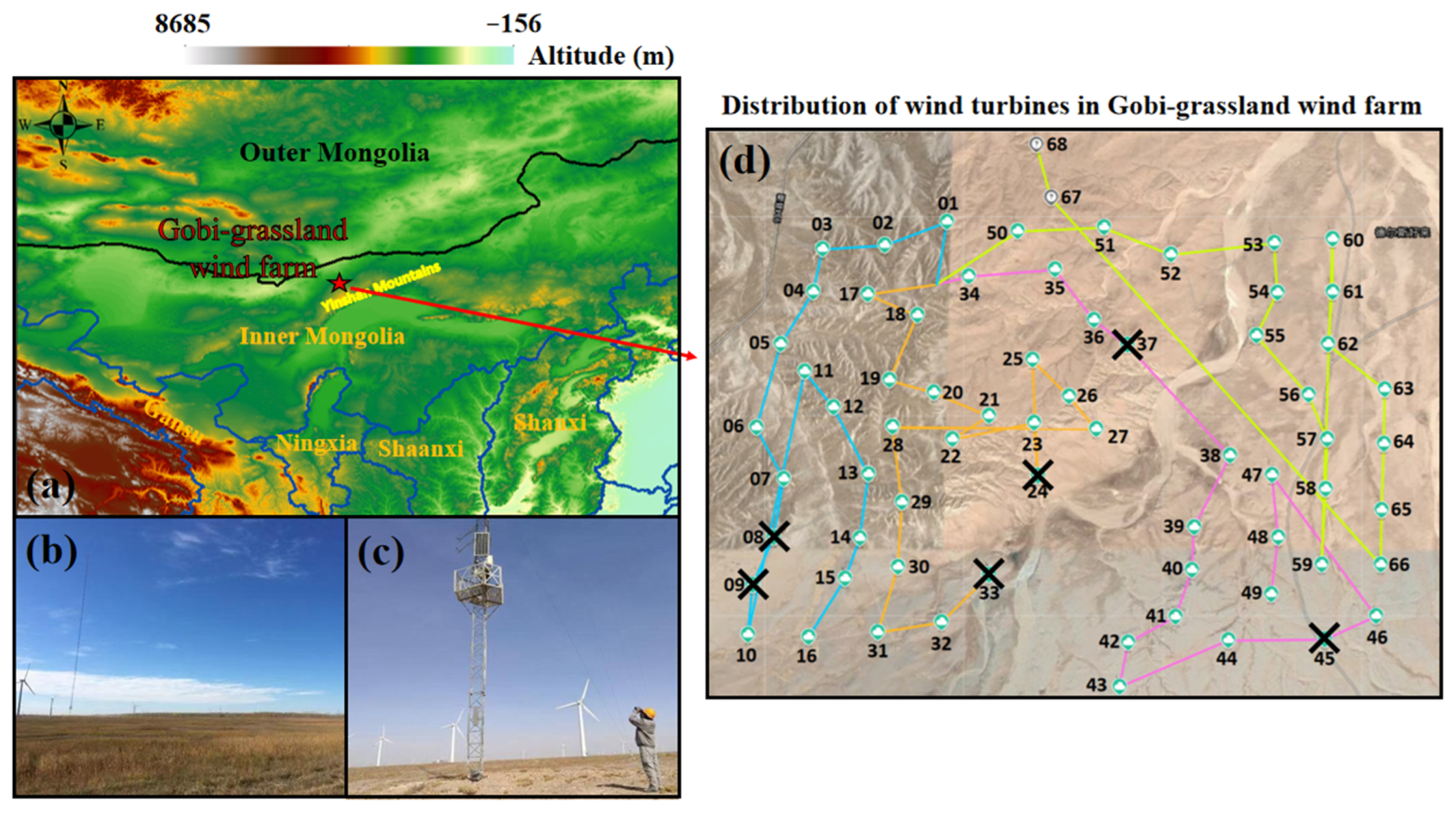
The Gobi grassland wind farm (41.55° N, 106.99° E) was built north of the Bayannur city of Inner Mongolia in 2009, which is located in the Urat Gobi grassland at the northern foot of Yinshan Mountains, as shown in Figure 1a. This wind Farm has 68 turbines with a rated power of 1500 KW. A meteorological wind sensor was mounted behind the turbine hub to measure the wind at hub height. Among these 68 turbines, six numbered 08, 09, 24, 33, 37, and 45 were out of service, marked as “×” in Figure 1d. There were also some failures in Turbine 60, but it could still generate power.

Figure 1.
The geophysical location (a), pictures (b,c), and distribution of wind turbines (d) of the Gobi grassland wind farm. Symbol “X” in (d) denotes the turbines out of service now and the different colored lines represent the turbines group built in different time.
2.2. Weather Research and Forecasting (WRF) Model
The Weather Research and Forecasting (WRF) model is a mesoscale numerical weather prediction framework designed for operational weather forecasting and atmospheric scientific research [22,23,24,25]. Here we adopted version 4.2, which is a fully compressible and nonhydrostatic mode with an Arakawa C-grid in the horizontal direction and high-terrain following coordinates in a vertical direction by default. In general, the WRF model can not only be applied to the case simulation of realistic weather but is also widely processed in the forecast of wind speed and power.
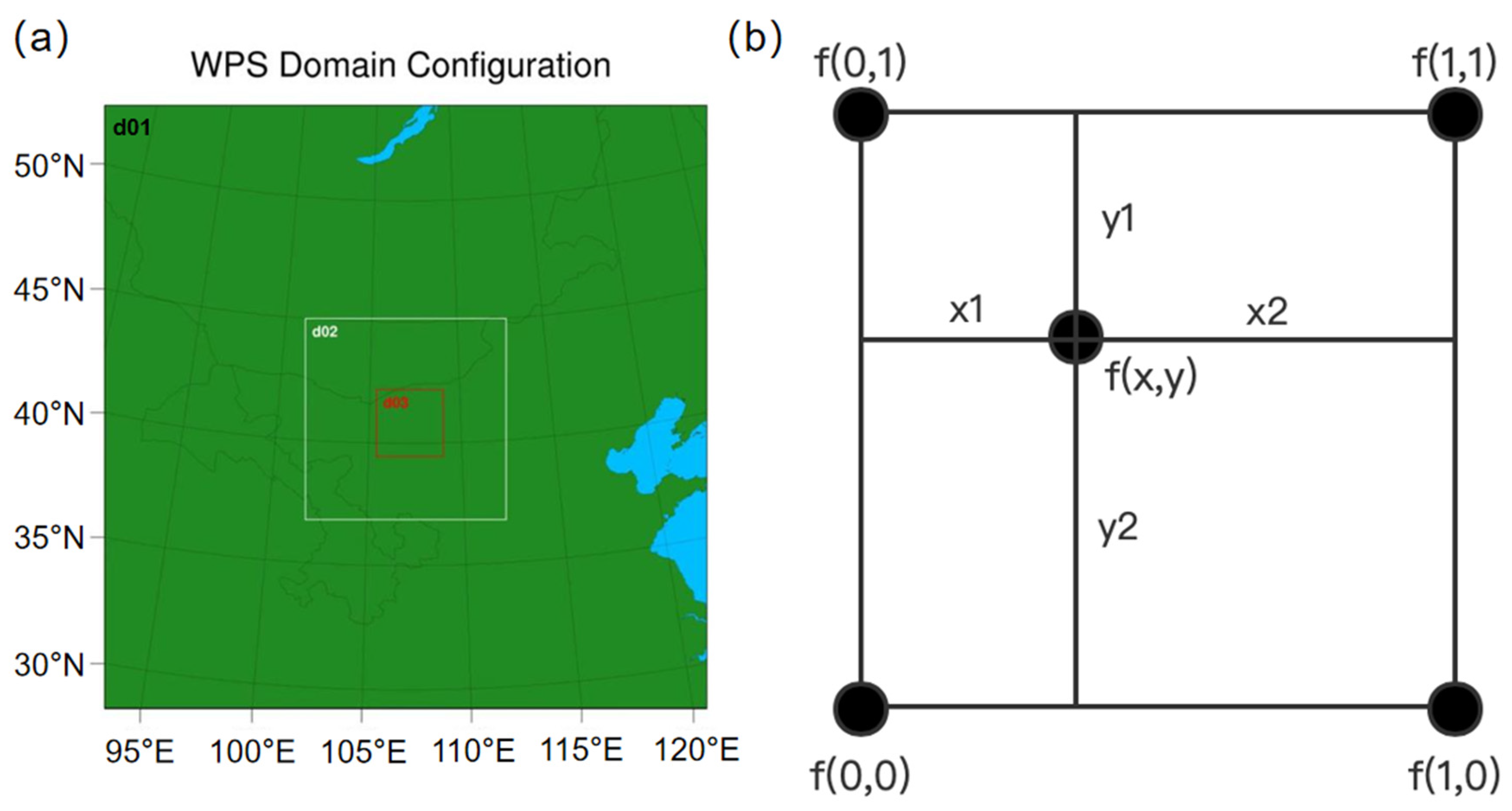
The simulation region was centered on (41.5° N, 107.0° E), and the three nested grid domains were designed with a spatial resolution of 27 km, 9 km, and 3 km, respectively, as shown in Figure 2a. The vertically layered encryption was 55 layers, and the top layer was 50 hPa. The parameterization schemes selected in this simulation are summarized in Table 1, in which the cumulus cloud parameterization scheme is disabled for Domain 03. For a detailed scheme introduction, please refer to Zhang et al. (2020) [23].
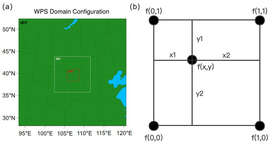
Figure 2.
(a) Schematic diagram of triple simulation domains of numerical WRF simulation and (b) schematic diagram of interpolation method.

Table 1.
Parameterization scheme of WRF model for the simulation of Gobi grassland wind farm.
A previous study has pointed out that the meteorological variables such as 10 m wind, sea–land terrain, surface net radiation, surface pressure, 10 m zonal wind component, 10 m meridional wind component, sensible heat flux, total column water vapor, 2 m dew point temperature, mean sea level pressure, and total cloud cover all have essential impacts on wind speed forecasting [26]. In addition to the influence of large-scale circulation, the boundary layer wind field is also affected by topographic relief, vegetation covers, as well as land use types. Simple smoothing operation of coarse-resolution model over terrains will produce potential errors in the boundary layer wind field, especially near the ground surface [27,28,29,30]. What is more, directly increasing the resolution of the model may lead to the complicated "gray zone" of boundary layer parameterization schemes, thereby generating more problems. In order to obtain a better result, the uses of mathematical statistics methods and artificial intelligence methods to learn the impact of terrain and other factors have been widely proposed for the postprocessing correction of wind speed.
2.3. Postprocessing Methodologies
2.3.1. Mathematical Statistics Algorithms
Bilinear Interpolation and Nearest Replacement
The output of WRF model simulations was stored in grid mode according to netCDF format. Since the grid position cannot precisely correspond to the turbine position, it is necessary to use the spatial interpolation method or replacement method to extrapolate and obtain accurate turbine position data. In this paper, bilinear interpolation and nearest replacement methodologies were adopted to process the data.
Bilinear interpolation is to estimate f(x,y) with the four nearest grid points (Figure 2b). By performing linear interpolation in the X direction first and then linear interpolation in the Y direction, we can obtain the final result of f(x,y). This interpolation output contains effective information on the four nearest grid points and will, therefore, be more representative and meaningful. More importantly, the computational efficiency is also reduced. The specific formula is as follows:
where x1 + x2 = 1 and y1 + y2 = 1.
The nearest replacement directly assigns the value of f(x,y) equal to the nearest grid point value, which has the advantage of higher computational efficiency compared with bilinear interpolation.
Average Variance–Trend (AVT) Method
The Average Variance–Trend (AVT) method was used to correct the wind speed calculated by bilinear interpolation and nearest replacement. This methodology, first proposed by Zhang et al. (2017) [31], de-trends both observational and simulated data series in the first step. Then, the two primary AVT parameters of average and variance of the two de-trending series are calculated. Finally, by correcting the average and variance of the de-trending simulated wind speed with an empirical equation [32], the corrected wind speed series can be obtained, which has the same average and variance as the observations. For a detailed introduction and specific equations of the AVT method, please refer to Zhang et al. (2018; 2019) [32,33].
Zhang et al. (2017) [31] applied the AVT method to three wind farms (Heiyazi wind farm, Machangshan wind farm, and Nanqiu wind farm) located in Gansu province. They found that the corrections based on AVT have satisfactory performance and result in an overall reduction in the forecast error rate of 30%. Recently, Han et al. (2022) [34] used this method to correct the prediction results of solar radiation forecast and reduce the bias effectively.
2.3.2. Machine Learning Algorithm
CatBoost, a categorical boosting algorithm, is a Gradient Boosting Decision Tree (GBDT) framework proposed on the basis of the Symmetrical Decision Tree algorithm, with characteristics of fewer parameters, class-based variables, and high accuracy. CatBoost solves the problems of gradient bias and prediction shift, thereby reducing the occurrence of overfitting and improving the accuracy and generalization ability of the algorithm [35,36]. Its advantages are:
- (1)
- It automatically treats categorical features in a special way. First, we make some statistics on categorical features and calculate the frequency of a certain category. Then we add the hyperparameter to generate new numerical features. With CatBoost, one no longer has to manually process categorical features;
- (2)
- CatBoost also uses composite category features to take advantage of the connections between features, which greatly enriches feature dimensions;
- (3)
- The method of Ordered Boost is used to avoid the deviation of gradient estimation and solve the problem of prediction offset;
- (4)
- The base model of CatBoost uses symmetric trees, and the method of calculating leaf value is also different from the traditional boosting algorithm. CatBoost has optimized calculating the average value and adopted other algorithms, all of which can prevent model overfitting.
3. Results
3.1. Wind Speed Distribution and Their Wake Effect
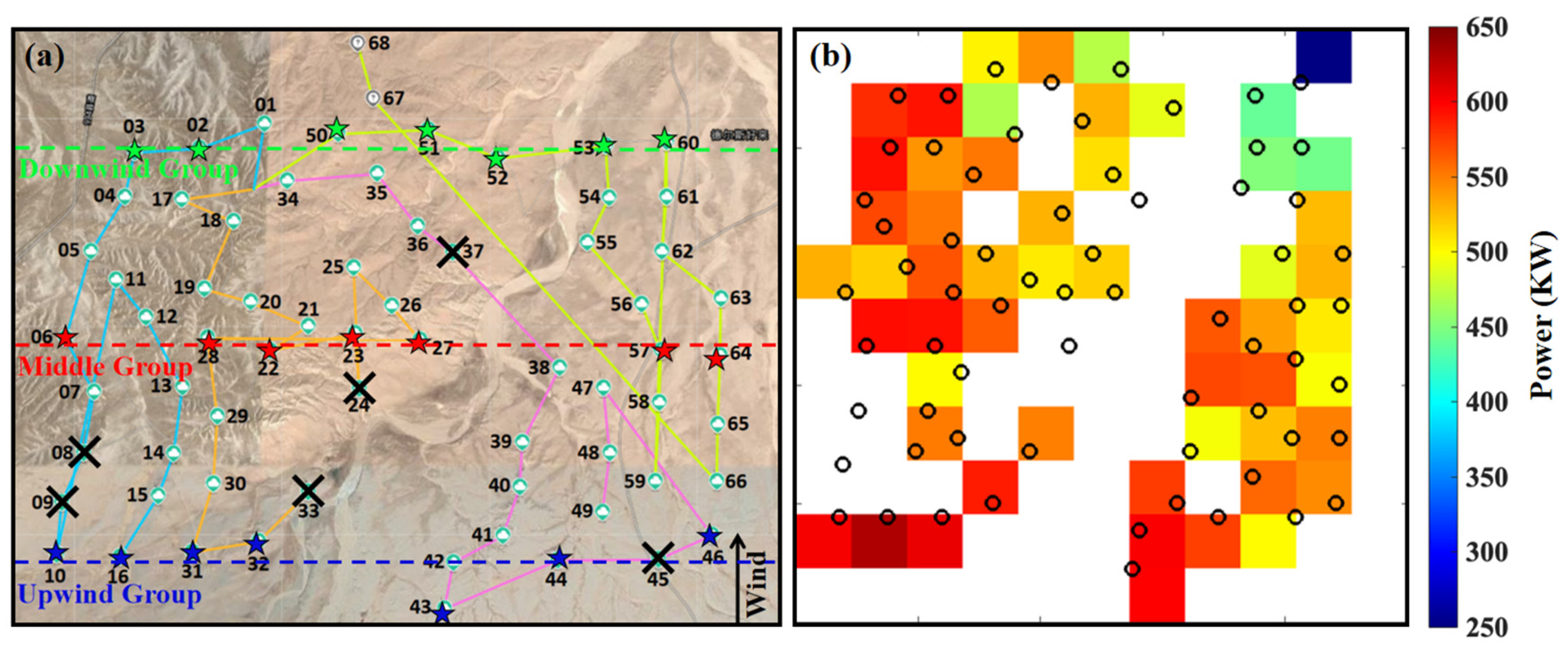
Analysis of the wind data observed on the turbines in September 2021 in the Gobi grassland wind farm shows that southerly wind dominates this area throughout the month, primarily distributed around 175–185°. According to this characteristic, we grouped these turbines into three categories along north–south wind direction, i.e., upwind group (Turbines 10, 16, 31, 32, 42, 44, and 46), middle group (Turbines 06, 22, 23, 27, 28, 57, and 64), and downwind group (Turbines 02, 03, 50, 51, 52, 53, and 60), shown in Figure 3a. By averaging the generated powers and wind speeds of the three groups, it is observed that the average power of the upwind group is 591 KW, with an average wind speed of 7.66 m/s, followed by 532 KW of the middle group (an average wind speed of 7.02 m/s), and 519KW of downwind group (an average wind speed of 6.92 m/s). The results indicated that the wake effects of the front turbines would significantly affect the generating capacity of rear-row turbines, with an average decrease of 12%.
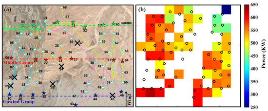
Figure 3.
(a) The grouped wind turbines along southerly wind in the Gobi grassland wind farm, with upwind group turbines 10, 16, 31, 32, 42, 44, 46, middle group turbines 06, 22, 23, 27, 28, 57, 64, and downwind group turbines 02, 03, 50, 51, 52, 53, 60. (b) Distribution of the average generated powers in September 2021.
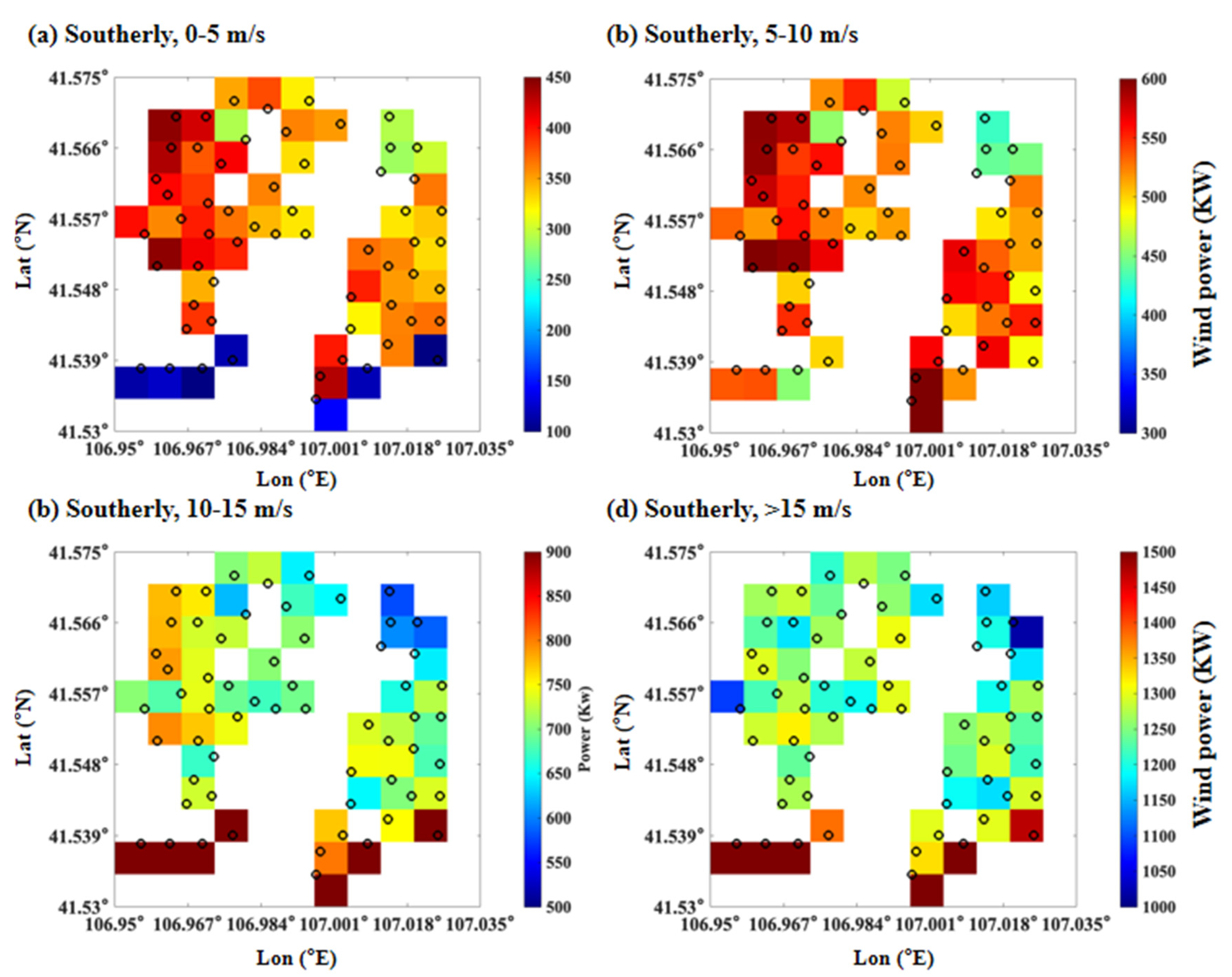
According to different wind speed regimes, the turbines are divided into four types: 0–5m /s, 5–10 m/s, 10–15 m/s, and >15 m/s, as shown in Figure 4 and Table 2. In Figure 4a, the occurrences of southerly 0–5 m/s wind accounted for 27.6%, with an average of generating power and wind speed in upwind direction of 368 KW and 5.90 m/s, respectively. The power and wind speed in the middle and downwind groups were 365 KW and 5.87 m/s, 118 KW and 3.65 m/s, respectively. By comparison, it is found that the wind wake effect significantly reduced the wind speed of the rear-row turbines, but the power generation of downwind turbines was higher than that of the middle group and upwind group, and the reasons for this phenomenon were not clear. In Figure 4b, the proportion of the conditions with the southerly wind of 5–10 m/s was 53.7%, and the downwind power and average wind speed were 523 KW and 6.97 m/s, respectively. The power and average wind speed of the middle and upwind groups were 537 KW and 7.03 m/s, 524 KW and 7.40 m/s, respectively. Results for the two scenarios indicated that in low wind speed conditions, the wake effect was not significant, and the powers generated by both front and rear groups were similar. In Figure 4c, the proportion of south wind 10–15 m/s was 16.7%, downwind power and wind speed were 688 KW and 8.17 m/s, smaller than 711 KW and 8.28 m/s in the middle group and 1283 KW and 11.83 m/s in upwind groups. It is observed that the increase in wind speed made the upwind wake effect more pronounced and the power generation in the rear row decreased by ~ 46%. In Figure 4d, the proportion of south wind >15 m/s was 2.0%. Upwind power and wind speed were 1494 KW and 16.16 m/s, respectively, higher than those of 1234 KW and 11.83 m/s in the middle group and 1234 KW and 11.77 m/s in the downwind group. At higher wind conditions, the wake effect perturbed by upwind turbines almost affected the whole wind farm, and the rear turbines could not reach full capacities.
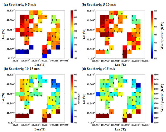
Figure 4.
(a–d) show the distribution of wind power of the Gobi grassland wind farm in groups of 0–5 m/s, 5–10 m/s, 10–15 m/s, and >15 m/s.

Table 2.
Statistics for the average generated power and wind speed of upwind, middle, and downwind groups in different southerly ranges of 0–5 m/s, 5–10 m/s, 10–15 m/s, and >15 m/s.
3.2. Wind Speed Correction Based on Mathematical Statistics Algorithms
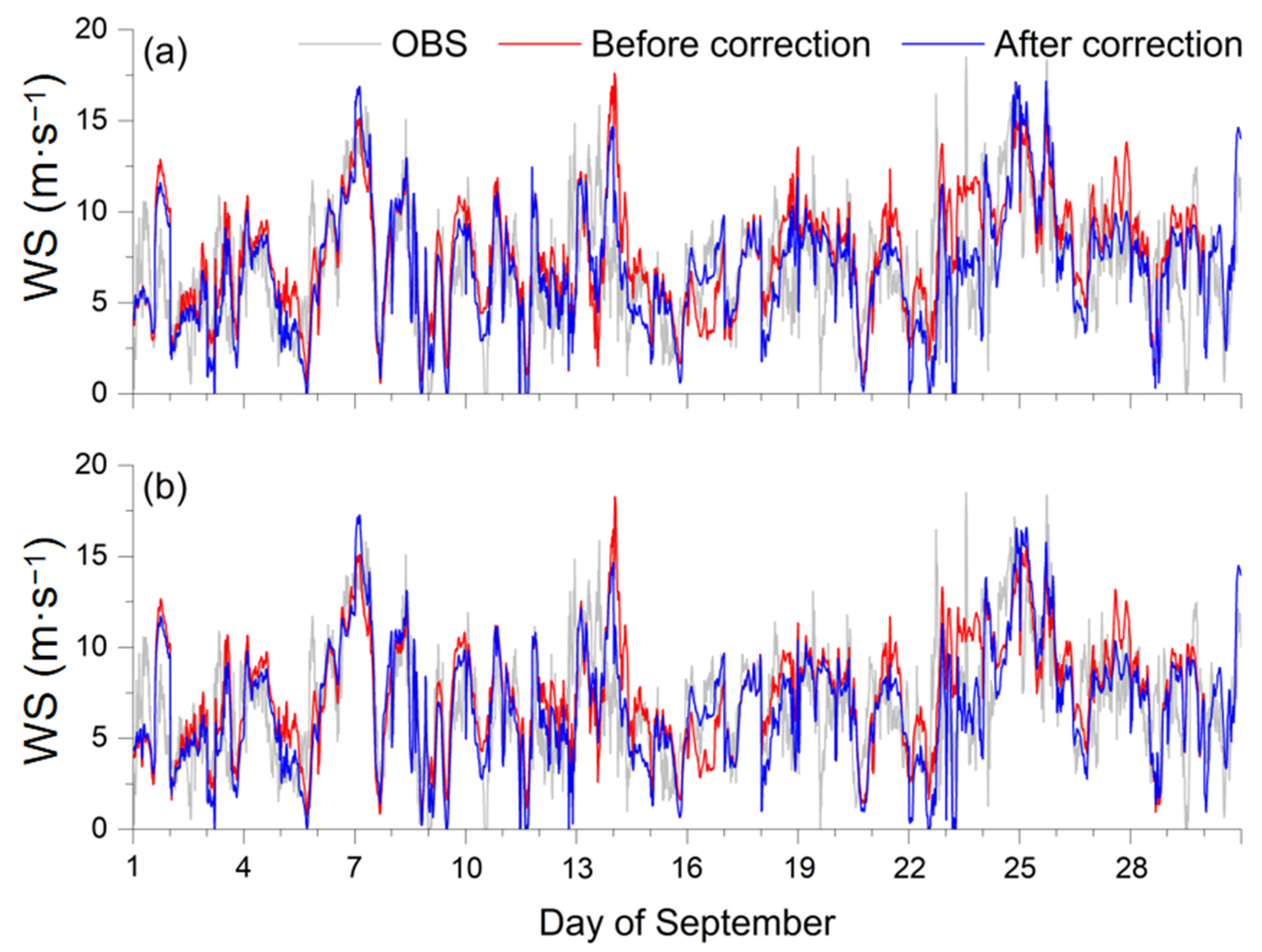
Figure 5 shows the deviation distribution of hourly WRF wind speed correction after bilinear interpolation and nearest replacement. Specifically, we used the observed and simulated data of turbines 06, 43, 50, and 64 for comparison. Intercomparison between WRF simulations and observations for the whole of September shows a root mean square error (RMSE) of 3.73 m/s. By postprocessing the WRF simulations with the two mathematical algorithms, we found that the two methods all exhibited great performance in presenting the trend of wind speed. The error of bilinear interpolation was reduced by 34.85%, and the average deviation was 2.43 m/s; in comparison, the nearest replacement method shows a much better result with a deviation of 2.38 m/s, decreasing by 36.19%. Results indicated that the implication of the adjacent turbine agreed better with observations than the multipoint interpolation. A possible explanation was that the adjacent wind turbines disturbed the local flow field and introduced more unknown errors, although this methodology introduced data from four grid points.
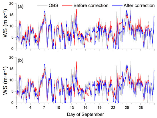
Figure 5.
Comparison between observational hourly wind speed (OBS, gray lines), WRF output (before the correction, red lines), and interpolation or replacement corrections (after correction, blue lines) of (a) bilinear interpolation and (b) nearest replacement.
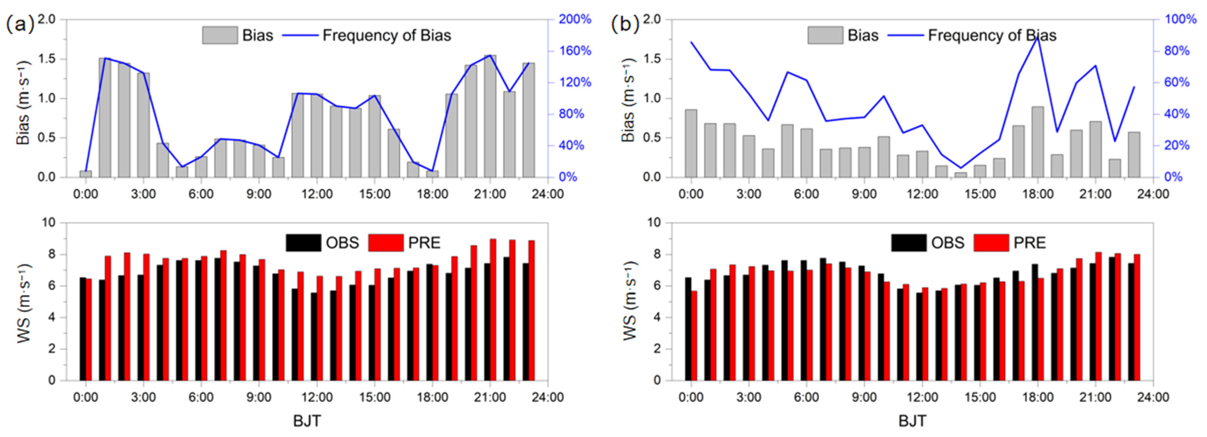
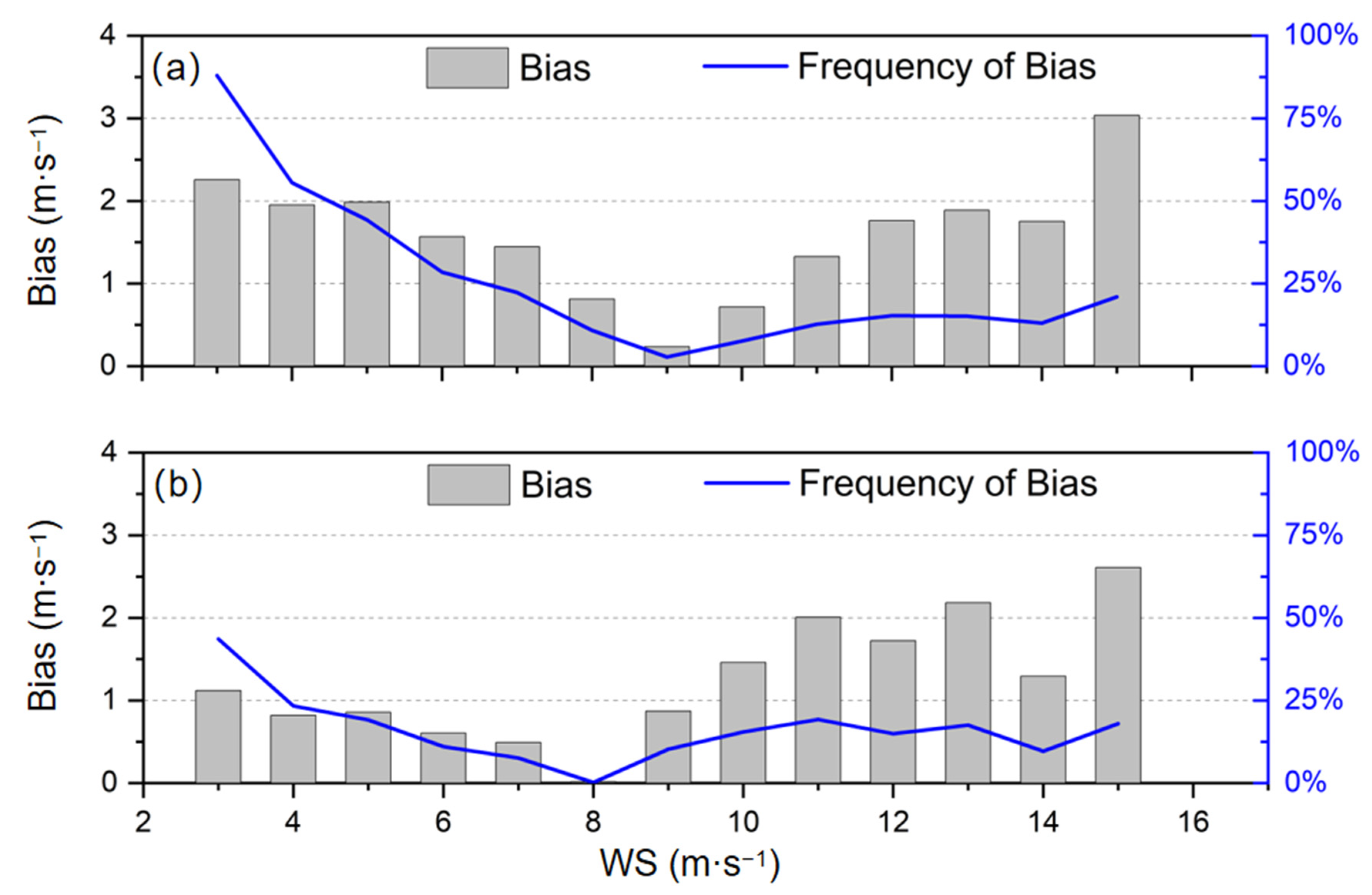
Considering the better performance of the nearest replacement, an AVT method was used to further correct its results (shown in Figure 6). Before the correction, there were three high deviation periods: 1:00–3:00, 11:00–15:00, and 20:00–24:00 after the evening. After processing the AVT corrections, the overall absolute deviation was significantly reduced. In Figure 7, it is observed that when the simulated wind speed increased to 8 m/s, the deviation decreased gradually as well. Whereas when the simulated wind speed continued to increase from 10 m/s, the deviation inversely started to increase [23]. Therefore, it is evident that the correction algorithm was able to make a great contribution in reducing the prediction deviation for the wind speed simulations smaller than 10 m/s, but for those beyond 10 m/s, the corrections were not so significant. In terms of real wind speed distribution, the samples with wind speed below 10 m/s accounted for as high as 86% of the total samples, much higher than that of high wind speed cases. It had a negative deviation of 41% and a positive deviation of 45%, showing no significant difference. Samples higher than 10 m/s accounted for only 14% of the total samples, including 10% negative bias and 4% positive bias, and the number of samples with negative bias played a dominant role. The cumulative wind power for the cases smaller than 10 m/s was 1.82 million KW, while the cumulative powers of the samples beyond 10 m/s was 1.24 million KW, indicating that the accuracy of high wind speed prediction was very important and needed to be further improved.
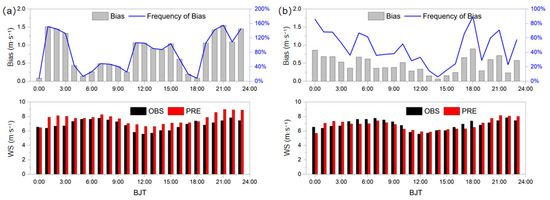
Figure 6.
Hourly wind speed correction of nearest replacement result using AVT methodology. Panel (a) is the result before AVT correction; panel (b) is after AVT correction.
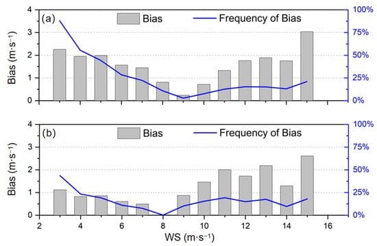
Figure 7.
Comparison of simulation deviations in different wind speed ranges after nearest replacement (a) before correction and (b) after correction.
In the AVT algorithm, the correction effect from the first day to the first 21 days was the best choice. In the experiment of this paper, historical data from 1–3 days and 12–15 days were used as cycles, which can achieve relatively good results. After rolling correction, the mean absolute error of wind speed after 1–3 days of cycle correction was obviously reduced. The margin of error was reduced by 10%. The error of the bilinear interpolation scheme decreased from 2.43 m/s to 2.14 m/s. The nearest replacement scheme error decreased from 2.38 m/s to 2.13 m/s.
The results show that the 15-minute deviation in simulation results can be corrected to the correct range at four different turbines, and the deviation of some periods can be significantly reduced. In the mid-latitude region, the near-stratum wind field mainly considers the large-scale dynamic effect, while Inner Mongolia is located in the region under the common influence of Mongolian cyclones, westerlies, and western Pacific subtropical high. Once there is an obvious deviation in the forecast of the location of the local weather system, the wind speed result is bound to have a large deviation [37].
3.3. Wind Speed Correction Based on CatBoost Artificial Intelligence Algorithm
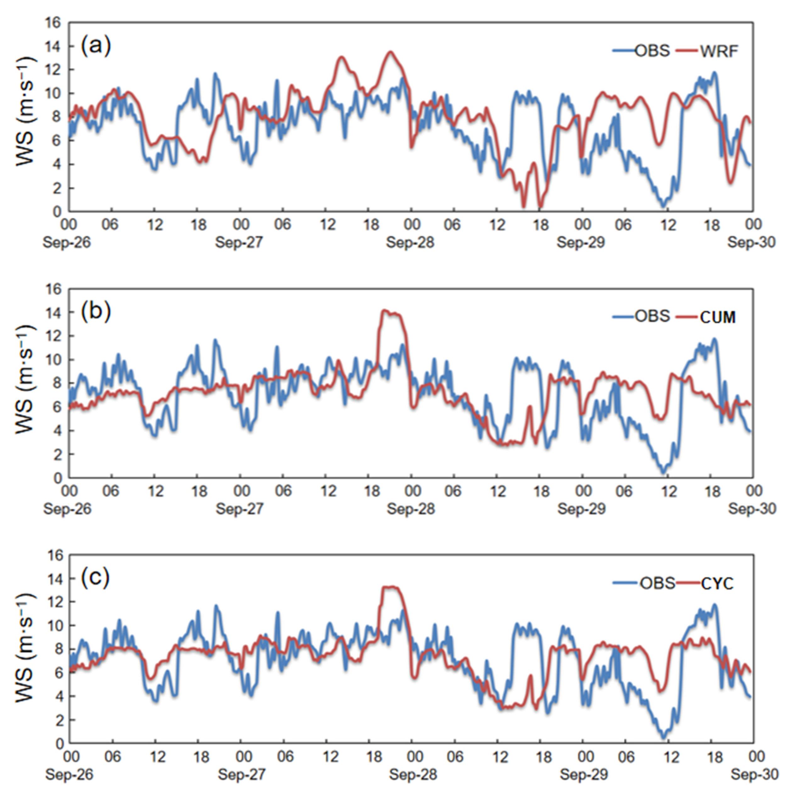
Two modes of cumulative learning method (CUM) and cyclic learning method (CYC) of the CatBoost artificial intelligence algorithm were used to correct the WRF simulation results, as shown in Figure 8. The CUM methodology means that all the datasets from before the prediction date serve as the training data for CatBoost, while in the CYC methodology, only the datasets with designated cyclic days prior to the prediction date are used for CatBoost training. In this study, for CUM methodology (Table 3), the data from 1 to 25 September were used for sample training, and the model prediction of the WRF-simulated wind field was based on 26 September data. Then, sample training was carried out using data from 1 to 26 September, and the prediction was made for 27 September. By parity of reasoning, the average RMSE of the wind field every 15 min is shown in Table 3. The correction has a better improvement on WRF forecast results. The four-day average RMSE can be decreased from 3.21 m/s to 2.55 m/s. For CYC methodology (Table 3), the 10-day data were designated for sample cyclic training; for example, 16–25 September data were used for sample training, and 26 September was used for model prediction; sample training was conducted from 17 to 26 September, and the model prediction was made on 27 September, and so on. The four-day average RMSE decreased from 3.21 m/s to 2.45 m/s. It is observed that the performance of the circular design is better than the sum correction. After testing the cycle of about 1–30 days, it was found that the cycle of about 10 days had the best performance, which is similar to the cycling scale of atmospheric circulation. Compared with the AVT output, it is observed that the four-day average of 2.55 m/s and 2.45 m/s of CUM_RMSE and CYC_RMSE showed a better performance than the 2.66 m/s of AVT_RMSE.
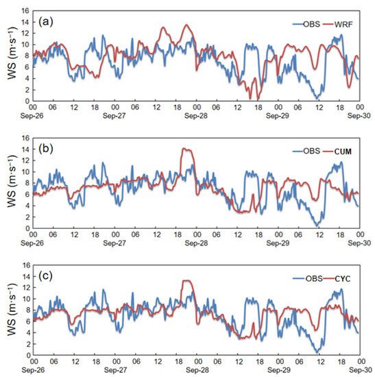
Figure 8.
(a) Turbine-observed (OBS) and WRF-simulated wind speed (WS, m/s); (b) turbine observed (OBS) and CatBoost_CUM-predicted wind speed (WS, m/s); (c) turbine observed (OBS) and CatBoost_CYC-predicted wind speed (WS, m/s).

Table 3.
Comparison of root mean square error (RMSE) between the simulated wind speed by WRF model (WRF_RMSE), CatBoost cumulative learning (CUM_RMSE), CatBoost cyclic learning (CYC_RMSE), and Average Variance–Trend (AVT_RMSE) during 26–29 September.
4. Summary, Discussions, and Outlooks
In this study, multiple approaches, including the mesoscale WRF model, mathematical statistics algorithms, and CatBoost machine learning algorithm, were adopted to explore the predictability of wind speed in the Gobi grassland wind farm in the Urat area of western Inner Mongolia. We found that the wake effect of front wind turbines significantly reduced the power generated by the rear-row turbines. The higher the wind speed is, the more pronounced the wake effect is on the rear-row group. The AVT postprocessing algorithm combined with bilinear interpolation and nearest replacement effectively optimized the WRF simulations, and CatBoost artificial intelligence algorithm also showed a good performance in reducing the errors of WRF output. However, under the influence of large-scale circulation, there are still relatively large deviations in the multi correction algorithms.
On the basis of these optimization results, we put forward the following suggestions as the main outlooks of this study:
- (1)
- Inner Mongolia is located in the region jointly affected by Mongolian cyclones, westerlies, and western Pacific Subtropical high, so the data assimilation of the northwest and Mongolian plateau should be strengthened in order to improve the simulation accuracy of wind speed;
- (2)
- In the boundary layer scheme, there are still major problems in parameterizing explicit variables of small-scale processes, and the results obtained by spatial interpolation or replacement methods not only have large deviations but may even cover the real values. Therefore, it is suggested that an optimized parameterization scheme should be proposed and constructed on the basis of the measurement of boundary layer structure over the underlying surface type and boundary layer structure in different seasons in the Gobi grassland landscape;
- (3)
- Local heterogeneous terrain has a pronounced influence on wind speed, and the terrain at wind power sites may have a potential impact on simulation results. It is therefore suggested to introduce high-resolution topographic data within the 30 km domain of the wind farm to improve the simulation precision of the near-surface wind field.
Author Contributions
Conceptualization, J.X., Y.M. (Yongjing Ma), and C.G.; methodology, J.X., Y.M. (Yongjing Ma) and C.G.; software, J.X.; validation, Y.M. (Yongjing Ma), Y.M. (Yining Ma) and C.G.; formal analysis, J.X. and D.B.; investigation, J.X.; resources, D.B. and S.Q.; data curation, D.B. and S.Q.; writing—original draft preparation, J.X., Y.M. (Yongjing Ma) and C.G.; writ-ing—review and editing, Y.J., T.P. and P.Y.; visualization, X.R.; supervision, J.X., Y.M. (Yongjing Ma) and C.G.; project administration, J.X.; funding acquisition, J.X., Y.M. (Yongjing Ma), C.G. and P.Y. All authors have read and agreed to the published version of the manuscript.
Funding
This study was supported by the Ministry of Science and Technology of China (2022YFF0802501), the CAS Strategic Priority Research Program (XDA23020301), the China Postdoctoral Foundation (2021M700140, 2022TQ0332), Gansu Natural Science Foundation (21JR7RA695), Northwest Regional Numerical Forecasting Innovation Team (grant number GSQXCXTD-2020-02), and the National Natural Science Foundation of China (41905053).
Data Availability Statement
Data are available upon reasonable request from the corresponding authors.
Conflicts of Interest
The authors declare no conflict of interest.
References
- Lu, X.; McElroy, M.B.; Kiviluoma, J. Global potential for wind-generated electricity. Proc. Natl. Acad. Sci. USA 2009, 106, 10933–10938. [Google Scholar] [CrossRef] [PubMed]
- Timilsina, G.R.; van Kooten, G.C.; Narbel, P.A. Global wind power development: Economics and policies. Energy Policy 2013, 61, 642–652. [Google Scholar] [CrossRef]
- Zheng, C.W.; Li, C.Y.; Pan, J.; Liu, M.Y.; Xia, L.L. An overview of global ocean wind energy resource evaluations. Renew. Sustain. Energy Rev. 2016, 53, 1240–1251. [Google Scholar] [CrossRef]
- Zheng, C.W.; Wang, Q.; Li, C.Y. An overview of medium-to long-term predictions of global wave energy resources. Renew. Sustain. Energy Rev. 2017, 79, 1492–1502. [Google Scholar] [CrossRef]
- Cherp, A.; Vinichenko, V.; Tosun, J.; Gordon, J.A.; Jewell, J. National growth dynamics of wind and solar power compared to the growth required for global climate targets. Nat. Energy 2021, 6, 742–754. [Google Scholar] [CrossRef]
- Wu, J.; Wang, Z.X.; Wang, G.Q. The key technologies and development of offshore wind farm in China. Renew. Sustain. Energy Rev. 2014, 32, 453–462. [Google Scholar] [CrossRef]
- Feng, Y.; Lin, H.Y.; Ho, S.L.; Yan, J.H.; Dong, J.N.; Fang, S.H.; Huang, Y.K. Overview of wind power generation in China: Status and development. Renew. Sustain. Energy Rev. 2015, 50, 847–858. [Google Scholar] [CrossRef]
- Zhang, S.J.; Wei, J.; Chen, X.; Zhao, Y.H. China in global wind power development: Role, status and impact. Renew. Sustain. Energy Rev. 2020, 127, 109881. [Google Scholar] [CrossRef]
- Dong, Y.; Liu, J.R.; Yang, J.X.; Ding, N. Carbon footprint of wind turbine by life cycle assessment. Acta Sci. Circumstantiae 2015, 35, 927–934. (In Chinese) [Google Scholar]
- Kang, Y.T.; Yang, Q.; Bartocci, P.; Wei, H.J.; Liu, S.S.H.; Wu, Z.J.; Zhou, H.W.; Yang, H.P.; Fantozzi, F.; Chen, H.P. Bioenergy in China: Evaluation of domestic biomass resources and the associated greenhouse gas mitigation potentials. Renew. Sustain. Energy Rev. 2020, 127, 109842. [Google Scholar] [CrossRef]
- Zhang, S.; Chen, W.Y. Assessing the energy transition in China towards carbon neutrality with a probabilistic framework. Nat. Commun. 2022, 13, 87. [Google Scholar] [CrossRef] [PubMed]
- Liu, H.; Tian, H.Q.; Chen, C.; Li, Y.F. A hybrid statistical method to predict wind speed and wind power. Renew. Energy 2010, 35, 1857–1861. [Google Scholar] [CrossRef]
- Wang, H.Z.; Li, G.Q.; Wang, G.B.; Peng, J.C.; Jiang, H.; Liu, Y.T. Deep learning based ensemble approach for probabilistic wind power forecasting. Appl. Energy 2017, 188, 56–70. [Google Scholar] [CrossRef]
- Wang, L.; Tao, R.; Hu, H.L.; Zeng, Y.R. Effective wind power prediction using novel deep learning network: Stacked independently recurrent autoencoder. Renew. Energy 2021, 164, 642–655. [Google Scholar] [CrossRef]
- Ren, Y.; Suganthan, P.N.; Srikanth, N. A novel empirical mode decomposition with support vector regression for wind speed forecasting. IEEE Trans. Neural Netw. Learn. Syst. 2014, 99, 1–6. [Google Scholar] [CrossRef]
- Wang, J.Z.; Hu, J.M.; Ma, K.L.; Zhang, Y.X. A self-adaptive hybrid approach for wind speed forecasting. Renew. Energy 2015, 78, 374–385. [Google Scholar] [CrossRef]
- Wang, J.Z.; Hu, J.M. A robust combination approach for short-term wind speed forecasting and analysis e combination of the ARIMA (autoregressive integrated moving average), ELM (extreme learning machine), SVM (support vector machine) and LSSVM (least square SVM) forecasts using a GPR (Gaussian process regression) model. Energy 2015, 93, 41–56. [Google Scholar]
- He, Z.S.; Chen, Y.H.; Shang, Z.H.; Li, C.H.; Li, L.; Xu, M.L. A novel wind speed forecasting model based on moving window and multi-objective particle swarm optimization algorithm. Appl. Math. Model. 2019, 76, 717–740. [Google Scholar] [CrossRef]
- Lin, Z.; Liu, X.L. Wind Power Forecasting of an Offshore Wind Turbine Based on High-Frequency SCADA Data and Deep Learning Neural Network. Energy 2020, 21, 117693. [Google Scholar] [CrossRef]
- Qu, Z.; Zhang, K.; Mao, W.; Wang, J.; Liu, C.; Zhang, W. Research and application of ensemble forecasting based on a novel multi-objective optimization algorithm for wind-speed forecasting. Energy Convers. Manag. 2017, 154, 440–454. [Google Scholar] [CrossRef]
- Qu, Z.X.; Mao, W.Q.; Zhang, K.Q.; Zhang, W.Y.; Li, Z.P. Multi-step wind speed forecasting based on a hybrid decomposition technique and an improved back-propagation neural network. Renew. Energy 2019, 133, 919–929. [Google Scholar] [CrossRef]
- Zhang, L.; Xin, J.Y.; Yin, Y.; Wang, Z.F.; Wang, D.W.; Ma, Y.J.; Jia, D.J.; Jiang, Y.Y.; Wu, L.; Pan, X.L. Adaptability evaluation of boundary layer schemes for simulation of sea and land breeze circulation in the west coast of the Yellow Sea. Atmos. Res. 2022, 278, 106354. [Google Scholar] [CrossRef]
- Zhang, T.J.; Zhao, C.L.; Gong, C.S.; Pu, Z.X. Simulation of Wind Speed Based on Different Driving Datasets and Parameterization Schemes Near Dunhuang Wind Farms in Northwest of China. Atmosphere 2020, 11, 647. [Google Scholar] [CrossRef]
- Zhang, T.J.; Li, Y.H.; Duan, H.X.; Liu, Y.P.; Zeng, D.W.; Zhao, C.L.; Gong, C.S.; Zhou, G.L.; Song, L.L.; Yan, P.C. Development and Evaluation of a WRF-Based Mesoscale Numerical Weather Prediction System in Northwestern China. Atmosphere 2019, 10, 344. [Google Scholar] [CrossRef]
- Skamarock, W.C.; Klemp, J.B.; Dudhia, J.; Gill, D.O.; Liu, Z.; Berner, J.; Wang, W.; Powers, J.G.; Duda, M.G.; Barker, D.M.; et al. A Description of the Advanced Research WRF Version 4; National Center for Atmospheric Research: Boulder, CO, USA, 2019. [Google Scholar]
- Sun, Q.D.; Jiao, R.L.; Xia, J.J.; Yan, Z.W.; Li, H.C.; Sun, J.H.; Wang, L.Z.; Liang, Z.M. A adjusting wind speed prediction of numerical weather forecast model based on machine learning methods. Meteorol. Mon. 2019, 45, 426–436. (In Chinese) [Google Scholar]
- Jiménez, P.A.; González-Rouco, J.F.; García-Bustamante, E.; Navarro, J.; Montávez, J.P.; Vilà-Guerau de Arellano, J.; Dudhia, J.; Muñoz-Roldan, A. Surface wind regionalization over complex terrain: Evaluation and analysis of a high-resolution WRF simulation. J. Appl. Meteorol. Climatol. 2010, 2, 268–287. [Google Scholar] [CrossRef]
- Jiménez, P.A.; Dudhia, J. Improving the representation of resolved and unresolved topographic effects on surface wind in the WRF model. J. Appl. Meteorol. Climatol. 2012, 2, 300–316. [Google Scholar] [CrossRef]
- Carvalho, D.; Rocha, A.; Gómez-Gesteira, M.; Santos, C. A sensitivity study of the WRF model in wind simulation for an area of high wind energy. Environ. Model. Softw. 2012, 33, 23–34. [Google Scholar] [CrossRef]
- Fernández-GonzáLez, S.; Martín, M.L.; García-Ortega, E.; Merino, A.; Lorenzana, J.; Sánchez, J.L.; Valero, F.; Rodrigo, J.S. Sensitivity analysis of the WRF model: Wind-resource assessment for complex terrain. J. Appl. Meteorol. Climatol. 2018, 3, 733–753. [Google Scholar] [CrossRef]
- Zhang, T.J.; Yan, P.C.; Li, Z.R.; Wang, Y.S.; Li, Y.H. A new cycle correction method for wind speed error in wind energy forecast based on short-term historical data. J. Arid. Meteorol. 2017, 35, 1042–1052. [Google Scholar]
- Zhang, T.; Yan, P.; Li, Z.; Wang, Y.; Li, Y. Bias-correction method for wind-speed forecasting. Meteorol. Z. 2019, 28, 293–304. [Google Scholar] [CrossRef]
- Zhang, T.; Yan, P.; Zhang, Z.; Duan, H.; Wang, Y.; Li, Y. Application of Various Technologies in Modification of Wind Speed Forecast in Wind Farms. J. Arid. Meteorol. 2018, 36, 835–844. [Google Scholar]
- Han, Z.; Yan, P.; Li, Y.; Lv, Q.; Zhang, T.; Bian, H.; Wang, Y.; Zhang, L. Study on correction of solar radiation forecast in Hexi region of Gansu Province based on short term historical data. J. Arid. Meteorol. 2022, 40, 125–134. [Google Scholar]
- Prokhorenkova, L.; Gusev, G.; Vorobev, A.; Dorogush, A.V.; Gulin, A. CatBoost: Unbiased boosting with categorical features. In Proceedings of the 32nd International Conference on Neural Information Processing Systems, Montréal, QC, Canada, 3–8 December 2018; pp. 6639–6649. [Google Scholar]
- Dorogush, A.V.; Ershov, V.; Gulin, A. CatBoost: Gradient boosting with categorical features support. arXiv 2018, arXiv:1810.11363. [Google Scholar]
- Wang, C.H.; Hu, J.; Jin, S.L.; Feng, S.L.; Liu, C. Application and test of lower level wind field simulation with meso-scale model WRF in western region of northwest China. J. Arid. Meteorol. 2011, 29, 161–167. [Google Scholar]
Publisher’s Note: MDPI stays neutral with regard to jurisdictional claims in published maps and institutional affiliations. |
© 2022 by the authors. Licensee MDPI, Basel, Switzerland. This article is an open access article distributed under the terms and conditions of the Creative Commons Attribution (CC BY) license (https://creativecommons.org/licenses/by/4.0/).

