Abstract
The parameters influencing the sea level measured with ultrasonic devices that are analyzed in this paper are the air temperature, atmospheric pressure and wind speed. As these variations are independent to each other and to the sea level, they can be removed from the measured sea level by applying a filtering algorithm based on independent component analysis (FastICA), adapted and improved for this application. The sound speed increases with temperature, so an internal temperature sensor is required to compensate for the sound-speed variation. Though this may improve the measurement accuracy, it is not enough to achieve the best results because there is a discrepancy between the internal sensor and the actual environment temperature. For high accuracy measurements, an external temperature sensor is required. In our case, we imported temperature datasets from a weather station, along with other datasets regarding atmospheric pressure and wind speed. The use of these external datasets, along with an algorithm based on principal component analysis (PCA) for error removal and the filtering algorithm based on FastICA for environmental phenomena extraction, allows us to achieve more accurate values for the Black Sea level in Constanta (2017–2020), independent of external influences.
1. Introduction
The sea level is considered one of the characteristic factors for the state of the marine environment. Its changes and influence decisively shape the coastal geomorphology and implicitly the position of the shoreline and therefore of the beach surface. The constantly rising sea level is a proof of the intensification of climate change, specifically of global warming [1,2,3]. Ocean level changes, melting glaciers and polar caps are key indicators of the global warming process. These effects will also increase the degree of risk for the coastal area of Romania. Several technologies are used for measuring the sea level: analogue measurements—stilling well gauges, pressure systems, acoustic systems and radar systems.
The stilling well gauge system involves a vertical tube with a diameter of about 1 m, made of concrete, steel or perforated plastic that, in isolated cases, is connected to the sea. Pressure systems measure the hydrostatic pressure of the water column and convert the measured pressure value into a level. For acoustic systems, the travel-time of a sonic pulse is used to calculate the distance to the sea. A stand-alone ultrasonic ranging system (SAURS) was designed and implemented to measure the water level in rivers, lakes and water reservoirs. Research has been focused on the problems associated with temperature correction and the results reveal a link between the temperature effect and its dependence on sound velocity in air [4]. Radar systems are similar to acoustic systems, but use radar frequencies. There are other direct measuring devices based on resistance or capacitance rods, but they are not widely used due to the lack of robustness required to make them suitable for hostile regions. Recent advances in technology, such as Global Positioning System (GPS) reflection methods, have led to other elaborate ways for sea level measuring. All these systems are currently being globally tested, and the results reveal a measurement accuracy close to 1 cm [4].
Based on LiDAR technology, time-of-flight (ToF) sensors use laser scanners and cameras to measure the depths of different points in an image by illuminating the scene with infrared light. ToF uses travel time to determine distance and depth. This is performed by using timed pulses for the transmitted waveform or by analyzing the phase shift of an amplitude modulated wave. Unlike other sensors, temperature does not affect travel time. However, when measuring the sea level, other environmental phenomena such as wind speed and atmospheric pressure need to be taken into account, because they influence not only the measurements but also the sea level directly. In the last years, research regarding sea-level measurements was performed using a variety of sensor systems. Ref. [5] proposed a cheap solution for marine water pollution detection, based on SRF05 ultrasonic sensors and an ATmega328p microprocessor, achieving a sensibility of about 1 mm. Ref. [6] used a combination of synthetic aperture radar interferometry (InSAR), GPS and tide-gauge observations to evaluate the sea-level rise in Tianjin, China. Radar technology was also employed by [7], who developed and tested a prototype radar system for sea-tide-level measurement, achieving a range resolution lower than 1 mm. In Romania, the Black Sea coast level is measured using a pressure sensor and a float gauge with a hydrometric view finder, also achieving an accuracy of 1 mm [8].
Following an international collaboration between the National Institute for Earth Physics (NIEP) and Joint Research Center (JRC), three ultrasonic stations were installed in the western part of the Black Sea regarding water level monitoring [9]. Our goal is to collect the measured Black Sea level data and process them by means of error correction and independent component analysis.
Independent component analysis (ICA) is a method used for multivariate signal processing. Given a mixed set of input vectors, it can estimate the independent signal sources. In previous work, we have used this method for a variety of applications, from voice blind source separation [10], to radar target classification [11] and electroencephalogram (EEG) signal processing [12]. We have shown, in these applications, that ICA will always yield the best results when the sources are independent or at least highly uncorrelated. For this reason, separating the external influences from sea-level measurements proves to be a great application for ICA. When evaluating the sea-level measurements, one can conclude that the measured level varies significantly, and that this variation is not periodic, being the result of a number of external influences other than tides. The external influences analyzed in this paper are temperature (seasonal), wind speed and atmospheric pressure. As these variations are independent to each other and to the sea level, they can be removed from the measured sea level by applying a filtering algorithm based on ICA. Regarding the processing method, there are a number of ICA algorithms (FastICA, JADE and Infomax) that perform the independent source estimations by following one of two general principles: maximization of non-Gaussianity and minimization of mutual information. In this paper, we will discuss the FastICA variant [13].
2. Materials and Methods
2.1. Problem Formulation for Sea Level Measurement Filtering
The National Institute for Earth Physics (NIEP) is responsible for the Romanian Black Sea coast water-level monitoring. The first network was installed within the Marine Geohazards project. In collaboration with the Joint Research Centre of the European Commission JRC, three stations were installed in the western part of the Black Sea (see Figure 1), within a project for the development of cheap devices for water-level measurements (inexpensive device for sea level measurements—IDSL) [14].

Figure 1.
Coastal seismic and Black-Sea-level monitoring network for the Romanian coast.
The inexpensive device for sea level measurements (IDSL) were developed in 2014 for sea-level measurement, in order to support the efforts of the Member States to improve the sea-level monitoring network. The IDSL measured the sea level using an HRXL-MaxSonar-WR ultrasonic sensor, model MB7363 produced by Maxbotix, MN, USA. The HRXL-MaxSonar-WR ultrasonic sensor is factory calibrated to match a narrow beam pattern and provides reliable long-range detection. The sensor has a full horn design and the most significant characteristics of this sensor are a 10 m range, an operating temperature range from −40 °C to 65 °C, 1 mm spatial resolution and a range resolution error less than 5 mm. The HRXL-MaxSonar-WR datasheet mentions that most range readings are accurately reported and if the range readings are affected, the effect is typically less than 5 mm. The IDSL devices’ performance, together with its low construction cost, makes it the ideal solution to cover many areas of the Mediterranean and Black Sea that need effective and reliable sea level measurements [15]. The ultrasonic sensor used by the IDSL device is placed over the water in order to measure the sea level. Pulses are sent periodically and the device measures the pulse travel time, duration that corresponds to the two-way distance between the ultrasonic sensor and water surface. The sea-level data used in our paper were measured with an IDSL device located in Constanța Port, near a cabin used for lighthouse operations. The Constanța IDSL device, that uses an HRXL-MaxSonar-WR ultrasonic sensor, is presented in Figure 2. The sea-level datasets measured in Constanța Port can be found on the WebCritech webpage, in the TAD (Tide gauge details) IDSL-19 database.
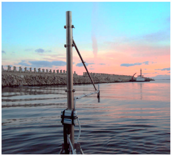
Figure 2.
Power subsystem mareograph.
The sea-level measurements are significantly influenced by sound velocity, which depends on environmental temperature. Thus, in order to achieve accurate sea-level measurements, the devices that collect the data from the ultrasonic sensors perform a software compensation for air temperature. This reduces the dependency between sea level and temperature. Current research reports that sound speed increases with 0.6 m/s per degree centigrade and that a one-degree-centigrade temperature variation may cause an error of about 0.17% in measured distance [4]. Though real-time knowledge of the environmental temperature may be useful in order to perform temperature compensation, the issue is that the temperature of the air path between the sensor and sea surface, especially closer to the water, may be different than the temperature measured by the device or the device Central Processing Unit (CPU)temperature, that are used for compensation. There are studies that report a correlation between the Rapsberry CPU temperatureand the error shift in sea level [15]. The Rapsberry Pi device is produced by Raspberry Pi Ltd., Cambridge, UK. However, this may not apply as a general rule and may yield erroneous sea-level compensated values, that will require further processing. Another issue is that environmental air temperature also increases the ultrasound signal attenuation, as it increases sound absorption through the air. This limits the distance between the sensor and water surface. The device we used in order to measure the sea level uses the temperature measured by the device and the CPU temperature in order to perform sea-level temperature compensation. As previously discussed, this may lead to erroneous sea-level corrections. Thus, we propose an alternative, more accurate, temperature source. The Vantage Pro2 system produced by Davis Instrument, Hayward, CA, USA used by a weather station, provides more accurate temperature measurements and also real-time data regarding other environmental phenomena, such as atmospheric pressure or wind speed, that may also affect the sea level. Histograms for the data collected with the Vantage Pro2 system are presented in Figure 3. These data were used for post-processing, in order to eliminate the influence of the environmental phenomena on the sea level.

Figure 3.
Environmental measurements from weather station Constanța.
Figure 4 presents the block diagram of the system proposed for real-time sea level measurements. Functionally, it can be structured in two main subsystems: a power subsystem and a processing subsystem that uses a Raspberry Pi development board. The Raspberry Pi collects the initial sea-level data values using the ultrasonic sensor. However, unlike most sea-level-measuring devices, this does not use the temperature measured by the device or the Raspberry CPU temperature in order to perform temperature compensation. Instead, the environmental-temperature data are collected from a weather station using the VantagePro2 system. The data collected from the weather station more accurately represent the air temperature within the path between the sensor and sea level. The values are used for temperature compensation that is performed during FastICA post-processing. The processed sea-level data are finally sent to a management unit for analysis and evaluation via an industrial router.
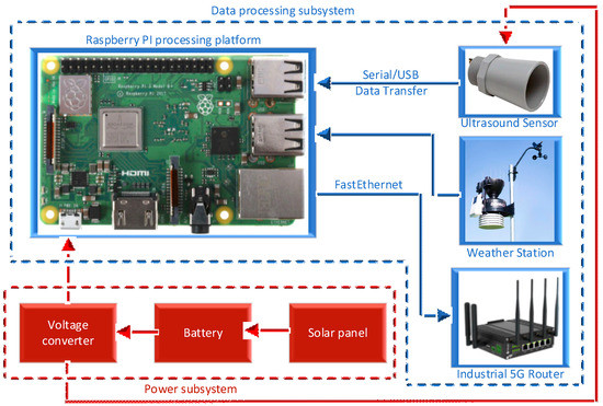
Figure 4.
Data processing and power subsystem mareograph.
2.2. Mathematical Method and Model for FastICA Filtering Algorithm
The purpose of the processing algorithm is to reject any influences atmospheric pressure, wind speed and, especially. temperature may have on the sea level measured in Constanța Port. The sea-level dataset, measured by the IDSL device, and the temperature, atmospheric pressure and wind speed, measured by the weather station, are fed subsequently as input features in the FastICA filtering algorithm. These input features are organized as the columns of an input data matrix X. Since we acknowledge the fact that there is a dependence between sea level and the other three input datasets, we can consider these vectors as linear combinations of some original independent sources, or the input data matrix as the multiplication result between the source matrix A we wish to discover and an unknown mixing matrix M:
The result of FastICA processing is the computation of a weight matrix W, that should be an estimate of M−1, which would allow us to estimate the source matrix.
First, the input matrix is pre-processed by subtracting the multivariate signal’s mean, and scaling the data so that each column vector of the input matrix has a variance of 1. These operations can be performed by applying principal component analysis (PCA) to the input data matrix. The mixed input vectors are projected by PCA onto a new set of orthogonal axes that maximizes the projected data. Thus, the pre-processed data matrix can be written as:
where X0 is the zero-mean input matrix, while V and D are the eigenvector and eigenvalue matrices. These matrices result from the eigen decomposition of C, the covariance matrix of X0:
The decorrelation results from the first multiplication performed in (2), while the second multiplication scales the variance to 1.
The first multiplication in (2) performs decorrelation, and the second multiplication scales the values of the projected data vectors so that each data vector has a variance of 1.
The contrast functions used in our FastICA implementation, and their corresponding derivatives are presented in (4) and (5). Parameter belongs to interval [1, 2], but is usually unitary.
The FastICA algorithm seeks to determine a number of weight vectors wi. These weight vectors will yield the coordinates corresponding to the unit vectors that form the multidimensional space in which the mixed datasets will be projected. The mixed datasets are the column vectors of Xw, and projecting these vectors onto the axes given by wi will yield the independent components. FastICA computes the weight vectors during an optimization process. Each vector is initialized randomly, and updated at each step according to:
The vectors are also scaled so that each has a norm of 1:
For each weight vector, the computation process stops when an error vector converges to zero. Each error value measures the similitude between the weight vector’s current values and its previous values, at each processing step. We considered that the error vectors converge to zero when two conditions are met. First, the final value of the error vector must be small enough. This threshold varies from one application to another, depending on how correlated the data vectors are, and needs to be chosen as a compromise between more accurate results and faster processing. In our case, we have established that a good convergence threshold is |ei| < 1 × 10⁻⁴. The second condition we imposed stated that the mean of the absolute deviations between the previous 100 errors had to be lower that the given threshold of 1 × 10⁻⁴. This ensures that obtaining a low error value is not by chance, but a result of convergence. We have also implemented a reset mechanism in our FastICA variant that automatically resets the weight vector to a new set of random values, if convergence is not achieved within a time duration of 1000 steps. Taking this into account, the algorithm computes a number of weight vectors equal the number of input features or columns of Xw.
Finally, the FastICA output matrix is computed by multiplying the pre-processed data matrix Xw with the weight matrix W that contains the previously computed weight vectors on its columns:
The columns of will represent estimations for the original sources. These will yield the sea level independent of temperature, atmospheric pressure or wind speed. Here we need to take into account the sign and order of the output components. The components’ order within the output matrix is random, and some components may be multiplied with −1.
After independent component estimation, we’ve evaluated the results by comparing the correlation of sea level with each environmental dataset before and after processing. The results are presented and discussed in Section 3.
The correlation between the sea level s[n] and another environmental dataset such as temperature t[n] was determined using:
The covariance, variance and standard deviation mentioned in (12) were implemented according to relations (10)–(12):
where N is the number of samples and is the mean of the sea level dataset s[n], defined by:
3. Results: Evaluation and Validation
After performing IDSL sea level measurements, signal processing is required: data decimation/interpolation (daily/monthly/yearly), error correction and additional statistical processing. The datasets were interpolated/decimated so that each month would have the same number of samples for all the input features measured by the ultrasonic sensor and weather station: sea level, atmospheric pressure, wind speed and temperature. Correction of the sea-level error caused by faulty ultrasonic measurements was achieved by applying an error correction algorithm based on principal component analysis (PCA). The PCA algorithm was fed the sea level measured for a certain month in each year. This removes significant magnitude spikes and any underlying noise present in the datasets. The results can be observed in Figure 5. The magnitude spikes may correspond to storms or seiches that are caused by strong winds and rapid changes in atmospheric pressure. The sea level deviations caused by seiches vary between a few centimeters to 2 m [16]. Though Black Sea storm frequency is generally low, the damage caused by these storms is significant, because the sea-level deviation caused by storm waves is seven to eight times greater than the deviations caused by common external influences. Figure 5 shows that after error correction, the maximum deviation in sea level is 1.0723 m. A similar deviation is reported by [17], that shows that the mean water level fluctuates widely in Constanța, from a maximum of 0.9 m to a minimum of −0.3 m, which yields a maximum deviation of 1.2 m.

Figure 5.
Error correction performed using a PCA-based algorithm.
After error correction, our goal was to separate any external influences from the corrected sea level dataset. Because the physical quantities that may affect the sea level are independent to each other and to the sea level, we chose to filter the corrected dataset using an algorithm based on independent component analysis (ICA). FastICA is applied in three stages, and its role is to subsequently remove the atmospheric pressure, wind speed and temperature components from the corrected sea level, in the specified order. During each stage, there are two input vectors for the FastICA algorithm: the current sea level, and either the variation of atmospheric pressure, wind speed or temperature, depending on the processing stage. FastICA will estimate the weights required to maximize the independence of the output vectors. Therefore, at the end of each stage the output vectors will be the external influence (atmospheric pressure, wind speed or temperature) and the filtered sea level, from which the external influence was removed. It is worth noting that for FastICA, the sign of the outputs is not important, so further processing is required after each stage. This includes sign correction and signal smoothing.
The first processing stage was the removal of atmospheric-pressure influence from the corrected sea-level dataset. This is shown in Figure 6. We can also observe that there is a reduction in atmospheric pressure during February 2017, that corresponds to the seiche present in Figure 5 as a magnitude spike.
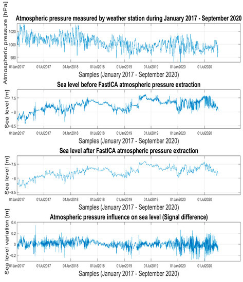
Figure 6.
Removal of the atmospheric-pressure influence on sea level using an ICA-based extraction algorithm.
The sea level resulting from the first stage is then introduced in the second FastICA processing stage, with the purpose of removing the wind-speed component from the sea level dataset. The results are presented in Figure 7. The algorithm detects similarities in the variations of sea level and wind speed and removes these similarities, in order to maximize independence. This is exemplified in Figure 7 with the removal of a magnitude spike cause by an increase in wind speed, during November 2017.
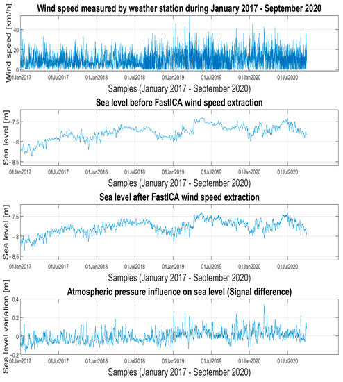
Figure 7.
Removal of the wind-speed influence on sea level using an ICA-based extraction algorithm.
The final processing and most important processing stage is the removal of temperature influence from the sea-level filtered dataset. Out of the three physical quantities analyzed, it seems that temperature has the most significant and visible influence on sea-level variation, during January 2017–September 2020. The results are presented in Figure 8.
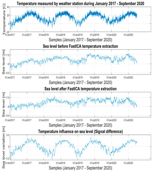
Figure 8.
Removal of the temperature influence on sea level using an ICA-based extraction algorithm.
4. Discussion
Figure 9 presents a three-dimensional comparison between the sea-level datasets, before and after processing, in relation to both temperature and time. The graphs on the right are two-dimensional projections generated with the purpose of showing the difference in correlation between sea level and temperature, as a result of FastICA processing. All graphs show seasonal temperature variation, but the 2D projections more clearly show that before processing, lower sea levels correspond to lower temperature values, independent of season. This dependence is corrected after processing and temperature component extraction from the sea-level dataset.
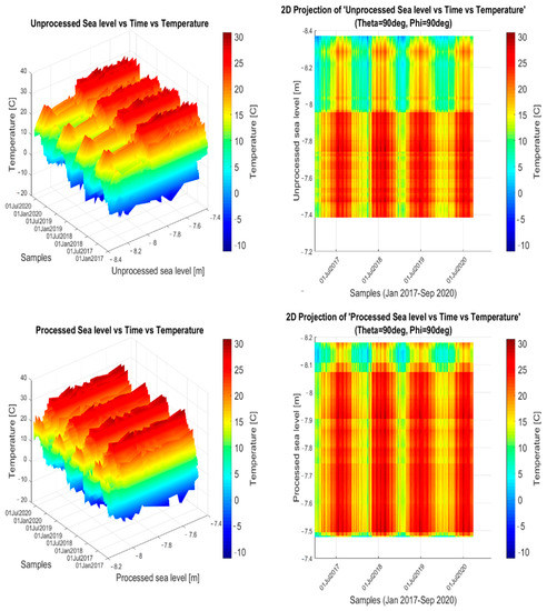
Figure 9.
Unprocessed and processed sea level vs. temperature during January 2017–September 2020.
Table 1 presents the sea-level standard deviation and its correlation to temperature, during each processing stage. The correlation coefficient computed for sea-level and temperature increases during the first two processing stages, due to the removal of atmospheric pressure and wind-speed components, that are independent and uncorrelated to temperature. Even though the sensor system used for sea-level measurements is configured to compensate temperature variation, the correlation coefficient computed before temperature component removal has a value of 0.5126 that indicates moderate correlation between temperature and sea level. After FastICA processing, the new correlation coefficient has a value of 0.0631. This value confirms that temperature influence has been extracted from the sea-level dataset. Furthermore, by removing external influences at each stage, the sea level tends to converge to a constant variation. The decreasing values of the sea-level standard deviation confirm this.

Table 1.
Sea-level processing results after each FastICA stage.
The scatter plots presented in Figure 10 show the difference in correlation between temperature and sea level, before and after FastICA processing. These graphs visually confirm the correlation results presented in Table 2.
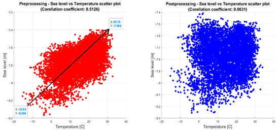
Figure 10.
Data whitening resulting from FastICA temperature influence removal.

Table 2.
The seasonal deviation from the multiannual sea level mean (January 2017–September 2020).
The processed sea level results were also analyzed from a seasonal perspective. The resulting means and deviations are presented in Table 2.
Before processing, one can observe that the sea-level mean is the lowest in winter and the highest in summer, due to its correlation to temperature. After processing, and temperature-influence removal, autumn seems to yield the lowest sea-level mean value. This result is confirmed by Ref. [18]. According to them, in autumn, especially during October-November, sea level is the lowest. These results also show that the sea-level variation decreases from one season to another. The seasonal variation decreases more than 50%, from a maximum of 0.1389 m (summer to autumn) to a maximum seasonal variation of 0.0689 m.
5. Conclusions
During January 2017–September 2020, sea-level measurements were performed in Constanța Port, using an ultrasonic sensor connected to a RaspberryPi device. The general issue regarding these types of measurements is that the measured sea level varies significantly, being influenced by a number of environmental phenomena, especially temperature. As temperature increases, sound speed increases and the travel distance of the ultrasonic pulse sent by the device is reduced. Though sea-level measuring devices perform temperature compensation, the results can be improved by processing the measured data. Another issue is that these devices do not take into account other external phenomena that may influence sea level.
The solution provided in this paper is to propose a multi-stage processing method that removes these external influences. This could only be achieved by acquiring other significant data regarding the aforementioned external influences. The physical quantities analyzed are atmospheric pressure, wind speed and temperature. Their variations during January 2017–September 2020 were provided by the Vantage Pro2 system, installed in a weather station located near Constanța Port. The processing algorithm first corrects any significant errors or amplitude spikes that may correspond to seiches or storms. Afterwards, the corrected sea level was processed in three stages, using an algorithm based on FastICA, improved for this application. We have imposed a convergence threshold of 1e−4 for weight vector computation and implemented a reset mechanism that reinitializes the weight vectors if convergence is not achieved within a time duration corresponding to 1000 iterations. FastICA was chosen as the processing method because the natural sea level, affected solely by tides and tributary discharge, and the physical quantities that influence it should be independent to each other.
The results show that by eliminating the external components, the sea-level standard deviation decreases after each processing stage, from a starting value of 0.1883 m to a final value of 0.1529 m. The results also show that the moderate correlation between temperature and sea level is corrected by extracting the temperature component from the sea level dataset. This is shown by the significant reduction in correlation coefficient computed for temperature and sea level. After FastICA temperature extraction, its value is significantly reduced from 0.5126 to 0.0631. This also affected the seasonal sea-level variations. After processing, the season with the lowest mean value for sea level was autumn, while for the initial unprocessed dataset, due to correlation to temperature, the lowest measured sea levels were during winter. The sea-level variation between season also decreases with about 50%, from 0.1389 m to 0.0689 m.
The processing algorithm based on FastICA proves to yield adequate results, which were verified by evaluating metrics such as correlation coefficient for sea level and temperature, sea level standard deviation and seasonal mean deviations. The proposed algorithm, with the required adaptations, may be implemented in real time, on the same system responsible for acquiring the sea-level data.
Author Contributions
Conceptualization, C.G.; data curation, C.G., L.T. and I.-A.M.; dormal analysis, C.G., L.T. and I.-A.M.; funding acquisition, I.-A.M.; investigation, C.G., L.T. and M.N.; methodology, C.G. and L.T.; project administration, I.-A.M. and C.I.; resources, I.-A.M. and C.I.; software, L.T. and M.N.; supervision, L.T., I.-A.M. and C.I.; validation, I.-A.M.; visualization, C.G. and L.T.; writing—original draft, C.G. and L.T.; writing—review and editing, I.-A.M. All authors have read and agreed to the published version of the manuscript.
Funding
This research was funded by: UEFISCDI, Phenomenal project, number PN-III-P2-2.1-PED-2019-1693 and MCI, Nucleu MULTIRISC program, project number: PN 19080102.
Institutional Review Board Statement
Not applicable.
Informed Consent Statement
Not applicable.
Data Availability Statement
The sea-level datasets measured in Constanța Port can be found on the WebCritech webpage, in the TAD (Tide gauge detailes) IDSL-19 database.
Acknowledgments
In addition to PN-III-P2-2.1-PED-2019-1693 and Nucleu projects that have funded the research, we thank to UEFISCDI PCE AFROS project, number P-III-P4-ID-PCE-2020-1361.
Conflicts of Interest
The authors declare no conflict of interest.
References
- Holgate, S.J.; Woodworth, P.L. Evidence for enhanced coastal sea level rise during the 1990s. Geophys. Reaseach Lett. 2004, 31, L07305. [Google Scholar] [CrossRef]
- Church, J.A.; White, N. A 20th century acceleration in global sea-level rise. Geophys. Res. Lett. 2006, 33, L01602. [Google Scholar] [CrossRef]
- Wenzel, M.; Schroter, J. Reconstruction of regional mean sea level anomalies from tide gauges using neural networks. Geophys. Res. Lett. 2004, 31, L07305. [Google Scholar] [CrossRef]
- IOC (International Ocean Commission). Manual on sea level, measurement and interpretation. UNESCO Man. Guides 2006, IV, 14. [Google Scholar]
- Rocchi, A.; Santecchia, E.; Ciciulla, F.; Mengucci, P.; Barucca, G. Characterization and Optimization of Level Measurement by an Ultrasonic Sensor System. IEEE Sens. J. 2019, 19, 3077–3084. [Google Scholar] [CrossRef]
- Tang, W.; Zhan, W.; Jin, B.; Motagh, M.; Xu, Y. Spatial Variability of Relative Sea-Level Rise in Tianjin, China: Insight From InSAR, GPS, and Tide-Gauge Observations. IEEE J. Sel. Top. Appl. Earth Obs. Remote Sens. 2021, 14, 2621–2633. [Google Scholar] [CrossRef]
- Nakazono, R.; Noda, R.; Kaneko, D.; Takeuchi, Y.; Kogi, Y.; Mase, A.; Ikezi, H.; Inutake, M. Development and Calibration of a Prototype Radar for Sea-Tide Level Measurement. In Proceedings of the 2018 International Conference on Engineering, Applied Sciences, and Technology (ICEAST), Phuket, Thailand, 4–7 July 2018; pp. 1–4. [Google Scholar] [CrossRef]
- Pérez Gómez, B.; Vilibić, I.; Šepić, J.; Međugorac, I.; Ličer, M.; Testut, L.; Fraboul, C.; Marcos, M.; Abdellaoui, H.; Álvarez Fanjul, E.; et al. Coastal sea level monitoring in the Mediterranean and Black seas. Ocean Sci. 2022, 18, 997–1053. [Google Scholar] [CrossRef]
- Annuntiato, A.; Galliano, D.A.; Bonaita, M. IDSL Sea Level Measurements Devices; JRC Tehnical Reports; Publications Office of the European Union: Luxembourg, 2016; pp. 1–56.
- Ghita, C.; Raicu, R.; Pantelimon, B. Implementation of the FastICA algorithm in sound source separation. In Proceedings of the 9th International Symposium on Advanced Topics in Electrical Engineering (ATEE), Bucharest, Romania, 7–9 May 2015. [Google Scholar]
- Tuţă, L.; Nicolaescu, M.; Roşu, G.; Grivei, A.; Bărbulescu, B. A Robust Adaptive Filtering Method based on Independent Component Analysis (ICA). In Proceedings of the 13th International Conference on Communications (COMM), Bucharest, Romania, 18–20 June 2020. [Google Scholar]
- Tuţă, L.; Roşu, G.; Popovici, C.; Nicolaescu, I. Real-Time EEG Data Processing Using Independent Component Analysis (ICA). In Proceedings of the 14th International Conference on Communications (COMM), Bucharest, Romania, 16–18 June 2022. [Google Scholar]
- Hyvärinen, A.; Hoyer, P.O.; Inki, M. Topographic Independent Component Analysis. Neural Comput. 2001, 13, 1527–1558. [Google Scholar] [CrossRef] [PubMed]
- Partheniu, R.; Ghita, C.; Toader, V.E.; Nastase, E.; Muntean, A.; Murat, E.; Moldovan, I.A.; Ionescu, C. Monitoring the black sea natural hazards using new technology and equipment. Rom. Rep. Phys. 2019, 71, 704. [Google Scholar]
- Annunziato, A. The inexpensive devices for sea level measurements. J. Tsunami Soc. Int. 2015, 34, 199. [Google Scholar]
- Niculescu, D.; Vlasceanu, E.; Mateescu, R.; Buga, L. Sea level variation at Constanța hydrology station. Bul. AGIR 2020, 3–4, 4. (In Romanian) [Google Scholar]
- Kuroki, K.; Goda, Y.; Panin, N.; Stanica, A.; Diaconeasa, D.I.; Babu, G. Beach erosion and coastal protection plan along the southern Romanian Black Sea shore. In Proceedings of the 30th International Conference on Coastal Engineering, San Diego, CA, USA, 3–8 September 2006. [Google Scholar]
- Vespremeanu, E.; Stroe, A.V.; Constantinescu, S. The Black Sea level oscillations in the last 150 years. An. Univ. Bucureşti–Ser. Geogr. 2004, 53, 69–76. [Google Scholar]
Publisher’s Note: MDPI stays neutral with regard to jurisdictional claims in published maps and institutional affiliations. |
© 2022 by the authors. Licensee MDPI, Basel, Switzerland. This article is an open access article distributed under the terms and conditions of the Creative Commons Attribution (CC BY) license (https://creativecommons.org/licenses/by/4.0/).