The Effect of European Climate Change on Indoor Thermal Comfort and Overheating in a Public Building Designed with a Passive Approach

Abstract

Dynamic building energy performance modeling is becoming increasingly important in the architectural, engineering, and construction (AEC) industry because of the sector’s significant environmental impact. For such analysis, a climate file representing a typical meteorological year (TMY) is needed, including hourly values for the most important weather-related parameters. However, TMY shows little resemblance to the future of the particular location where a building has been used for decades. Therefore, using predicted future climates during building design is unfortunately rarely practiced, potentially undermining the strategies that should be the fundamental basis of the design. To explore this question, our study compared the heating and cooling energy consumption, indoor thermal comfort, and summer overheating potential of a selected building for three distinctive European climates, in Hungary, Portugal, and Lithuania. All of them were changed according to the IPCC RCP4.5 scenario, and were examined for the present, the 2050, and the 2100 scenarios. We also tested adaptive clothing to evaluate the indoor comfort parameters. The results show a 10% increase in heating and cooling energy use for the same construction and location between 2020 and 2100. The continental climate of Budapest is the most threatened by summer overheating, with an increase of 69% for the ODH₂₆ indicator. A more balanced warming for Lisbon was found (23%), and moderate changes for the city of Kaunas (a 153% increase from a very low baseline).

1. Introduction

Numerical simulation of our designed buildings and of their energy performance is becoming increasingly important nowadays in the architectural, engineering, and construction (AEC) industry to mitigate its harmful effects. Not only is the AEC sector responsible for approximately 40% of the waste produced on Earth, but also accounts for a similar portion in terms of energy consumption and carbon emissions. In a study focusing on India, Raj et al. summarized the importance of systematically optimizing the building performance by simulation tools [1]. By getting a detailed overview of the energy consumption of each system and the building envelope’s most important parameters, such as heat flow or surface temperatures, it becomes possible to assess user thermal comfort, indoor air quality, and total energy consumption. It is clear that the design of a space is not a single target exercise, thus multi-objective optimization is required for any meaningful and well-planned space, be it public [2] or residential [3]. The aim of providing good IAQ (indoor air quality) with low energy consumption is not only a problem for contemporary building owners and users [4] but for future cases too. With measurement data available from the past, the validation of simulation results is possible, and is necessary to calibrate a model [5]. Still, the uncertainties of the future are challenging to predict accurately in terms of occupancy [6], yet substantially governs all the assessed parameters. With the changing climate, which is shifting the generally comfortable European weather into a more extreme one, not only do we need to adapt our building strategies, but we also need to consider the concerns against the metrics that we use to quantify thermal comfort. According to the study of Picard et al. [7], weather is one of the most significant factors influencing energy consumption and thermal comfort in our buildings—yet its variation is usually not taken into consideration among the six criteria listed by Yoshino et al. [8]: (1) weather, (2) building envelope, (3) building energy and services, (4) indoor design criteria, (5) building operation and maintenance, (6) occupant behavior. Not taking climate change effects into account makes the buildings vulnerable to it [9]. Ruijun et al. carried out a sensitivity study considering the effects of 25 input parameters on office buildings: their study emphasizes the general importance of the building envelope, heating and cooling setpoints, and infiltration [10]. Other issues are present in the practice of energy simulation. For example, numerous critiques targeting the PMV & PPD method developed in Denmark by Fanger in the 1970s [11] derive from warmer climates questioning its applicability. Hwang et al. describes their concerns in [12], referencing, e.g., Pereira and Broday, who made an attempt to somehow correct PPD (predicted people dissatisfied) to APD (actual people dissatisfied) [13].

Running dynamic building energy simulations are becoming standard in the AEC industry, with larger projects requiring certifications such as LEED [14], BREEAM [15], DGNB [16] or WELL [17]. These compliance modeling exercises are not always a design tool; they measure the as-designed or as-built state against the chosen metric described in the credit description. This usually refers to one of the international de-facto standards, ASHRAE 90.1 [18], which defines a detailed instruction set to build a dynamic energy model. ASHRAE 90.1’s Appendix G in Table G2.3 states that “The simulation program shall perform the simulation using hourly values of climatic data, such as temperature and humidity from representative climatic data, for the site in which the proposed design is to be located. For cities or urban regions with several climatic data entries, and for locations where weather data are not available, the designer shall select available weather data that best represent the climate at the construction site. The selected weather data shall be approved by the rating authority” [18]. For dynamic simulations, a file containing sufficient input weather data is required with hourly values for the most important parameters such as external temperature, diffuse and direct solar radiation, relative humidity, and wind direction. The approved weather files are usually typical meteorological years (TMY), composed of many measured data points from the past. EnergyPlus accepts a wide range of formats [19]. Building energy modeling (BEM) is about predicting the future; thus, it requires a great understanding of what might happen with the given climate in the future. Indeed, previous research highlights that both the RCP4.5 and RCP8.5 scenarios will result in a significant decrease in HDD (heating degree days) and an increase in CDD (cooling degree days) in Portugal [20], but will result in a decrease in both metrics in Canada [21]. Climate prediction is a very complex topic. It is impossible to accurately anticipate how each location is going to respond in the upcoming decades, yet we tend to design buildings according to experience and global precedents.

The research question of this paper explores the topic of climate data used for dynamic building simulations in the context of global climate change: if we do use historical data to design the buildings for the future, how reasonable are these assumptions? Will the designed specifications hold up in a changing climate, or should it be the norm to use modified climate data according to climate change scenarios?

The case study building serves as the analysis base to explore the impacts of the changing European climate on human thermal comfort. Three cities were chosen in significantly different climates to see how adapting them according to the Intergovernmental Panel on Climate Change (IPCC) extrapolated scenarios affects the humans using the space. There is research to be found regarding the topic, mostly focusing on a specific climate and the changes in that location over time. The study of Ahmadian et al. assessed the current and 2050 climates of London and predicted a significant increase for energy consumption in all building typologies and geometrical configurations [22]. A similar analysis was done by Ruiz and Olmo [23] for the Spanish climate, concluding that according to the RPC 4.5 scenario, nearly zero energy buildings (nZEB) are reliable for the changing climate. Farahani et al. assessed the overheating risk and energy demand of new and old apartment buildings in Finland [24], concluding that in the future Nordic climate, passive means of ventilation will not be sufficient to prevent overheating in our buildings. In our literature review, we did not find any article that compares the same building across various climates. We find these questions important because the AEC sector is a global and commercialized industry, in which buildings built across the globe tend to share very similar technical specifications and operational qualities.

2. Methods and Materials

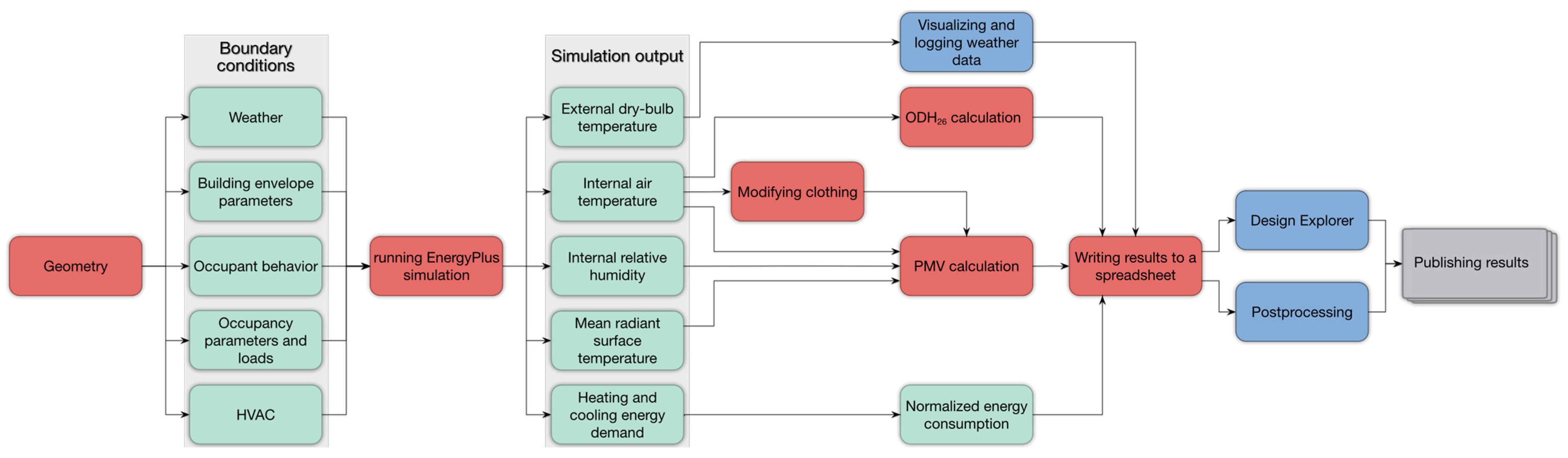
2.1. Methodology

The design of the analyzed public building was supported by parametric dynamic energy modeling and daylight studies to determine appropriate glazing for the external envelope based on the evaluation of internal comfort parameters [25] as described on the flowchart in Figure 1. The flowchart describes the internal logic of the developed Grasshopper script which creates the building energy model and runs the simulation in EnergyPlus.

This was done by using the climate file representing the current typical meteorological year of Kaunas, downloaded from the US Department of Energy’s (DoE) database with the help of EPW Map [26]. The file used is the KAUNAS: 266290: IWEC (International Weather for Energy Calculations). The IWEC data files are ‘typical’ weather files suitable for use with building energy simulation programs for 227 locations outside the USA and Canada, and are the result of the American Society of Heating, Refrigerating and Air-Conditioning Engineers’ (ASHRAE) Research Project 1015 conducted by Numerical Logics and Bodycote Materials Testing Canada for ASHRAE Technical Committee 4.2 Weather Information [19].

A comprehensive building information model (BIM) was built in ArchiCAD that served as the source of the whole documentation and the basis of the design tasks. With a conversion of this model to a building energy model (BEM), we faced common challenges [27], and several workflows were tested to ensure the least amount of lost data. We opted to use open source tools mainly because they provide access to their inner algorithms. Our research showed that the method described in this paper (summarized in Figure 2) is a less common approach used by professionals who, in practice, use either Revit or AutoCAD as their main source of the geometry [28].

In this way, it was possible to evaluate the model progression at every step. This proved to be useful, as significant simplifications needed to be applied: the starting model was far too detailed to be useful in a building energy simulation. The most problematic aspect came from the fact that most parts of the thermal envelope were modeled by numerous disconnected elements instead of using composite profiles—a data structure that enables the definition of multi-layered skins in a building model as one element.

The whole building energy model is composed of 42 zones, the simulation, and management of which are beyond the scope of the exercise. We chose a single south-facing space, for which user comfort is paramount. The selected space under study is the first-floor library (room 103). Its large east, south, and west-facing windows make it a good study subject. The function was modeled using the “SecondarySchool::Library” operational program described in ASHRAE 90.1:2019 [18], with the Occupancy schedule modified to 07:00–19:00.

Single zone BEM was used to analyze the chosen single space in the building, which is a largely glazed, externally and internally shaded, south-facing library room. Its geometry reflects the current trends in contemporary architecture, using as much glazing as financially possible to create visual connections with the external world. We used single zone analysis to gather an understanding of the effect of changing only certain parameters of the thermal envelope instead of using whole building simulation to assess the total energy demand of the design. EnergyPlus was chosen as the simulation interface because of its widely validated and open source nature. To easily parameterize the building, we chose Ladybug Tools (LBT) [29] as the interface to create the parametric model with the help of Grasshopper in Rhinoceros 3D. Choosing this approach made it possible to couple the simulation engine with other Grasshopper plugins, such as Colibri (part of the TT Toolbox set of custom nodes [30]), to capture all the information as a result of automated parametric runs and showcase them via an open source web-based viewer called Design Explorer, providing interactive ways to filter and assess the results. This framework is common and used to parameterize and assess a well defined design space; for example, Shao et al. employed a similar approach to designing a building skin according to multiple criteria [31]. The interactive viewer can be accessed via the link in [32]. We recommend following the same approach to build cohesive toolkits on top of the available open source simulation engines tailored to the task [33]. Such a custom tool can be seen in Figure 3, which is our implementation of the framework described in Figure 1, with each color marking a distinctive module for a specific function.

2.2. Evaluation Indices

2.2.1. Heating and Cooling Energy

No changes were made to the heating, ventilation, air conditioning system (HVAC) or the lighting in the compared options, thus only the heating and cooling energy were compared to achieve greater clarity in the result assessment. The heating and cooling energy indicated is the electric energy required to operate the heat pumps assumed in the building, and from this, we calculated the normalized annual amount of energy (kWh/m²a). The reason for normalizing energy consumption by dividing the total energy use by the usable area is to receive a unitized value which can be compared against similar buildings and standardized values.

2.2.2. Thermal Comfort—PMV

For evaluating comfort metrics in the building, various methods could be used: predicted mean vote (PMV) is used to assess the comfort in mechanically heated and cooled buildings which gives the percentage of people dissatisfied (PPD), a method which was developed by Fanger [11]. PMV is an index that predicts the mean value of the thermal sensation votes (self-reported perceptions) of a large group of persons on a sensation scale expressed from −3 to +3 corresponding to the categories “cold”, “cool”, “slightly cool”, “neutral”, “slightly warm”, “warm” and “hot” [34]. PPD is an index establishing a quantitative prediction of the percentage of thermally dissatisfied people determined from PMV [34]. The critical assertion of PMV led to the adaptive model introduced to the ASHRAE 55 standard in 2004, as it is a better metric for naturally ventilated buildings. The adaptive model relates indoor design temperatures or acceptable temperature ranges to outdoor meteorological or climatological parameters [34], and it is generally considered a better metric for naturally ventilated spaces [35]. Using ISO 7730 [36] comfort classes enable a rapid evaluation of a space on an annual basis: it allows the classifying, on an hourly basis, of the percentage of time that the room in question is occupied in each class, the result of which is stored in a database. In the SQL database, the PMV value describing the thermal comfort is available for all rooms in the building on an hourly basis. The classification based on PMV values can be done as follows: Class A if |PMV| ≤ 0.2, Class B if 0.2 < |PMV| ≤ 0.5, Class C 0.5 < |PMV| ≤ 0.7, and Class D |PMV| > 0.7. This logic was implemented in Grasshopper, as shown in Figure 4. The metric used for the annual evaluation was calculated according to the above relationship, which gives the percentage of the year in which the tested room is in a particular class. The ideal condition is when ν_A = 100 %. For the required inputs for the PMV calculation, the clothing insulation levels were adjusted with the method described in the previous section.

2.2.3. Summer Overheating—ODH

When evaluating summer overheating within homes, the exceedance of fixed absolute values is generally used [37,38]. The overheating criterion is usually defined at 26 °C most cases [39,40]; CIBSE (Chartered Institution of Building Services Engineers) indicates that bedroom temperature should be maximized at 26 °C since sleep quality and thermal comfort decrease when the temperature rises above 24 °C [36]. In our analysis, we used this threshold and the ODH₂₆ indicator to evaluate the overheating of the analyzed building. This indicator stands for “Overheating Degree Hours above 26 °C”, which considers not only the hours above the threshold but the extent of the overheating as well (measured in Kh/a, i.e., Kelvin hours/year). Since there are some differences between the weather conditions studied, especially in Lisbon, which has mild winters and a relatively warm transition period, a specific, identical period (15 October to 15 April) was chosen for the analysis. The calculation logic is captured in Figure 5 (which is a snippet from the complete script shown in Figure 1), using the EnergyPlus air temperature outputs and hour of the year (HOY) indices to isolate the analyzed period. In the simulations, generated weather files were used, where the contemporary data included measurements from the past 20 years, and future scenarios were generated based on the IPCC report 2014 “intermediate” RCP4.5 scenario [41]. It is an intermediate stabilization pathway, where the projected mean global mean surface temperature change, compared to the 1986–2005 period, is 1.4 °C for the 2046–2065 period and 2.2 °C for the 2081–2100 period.

2.3. Case Study Building

The building design chosen for the parametric assessment of the thermal condition and indoor air quality (IAQ) parameters in contemporary and Representative Concentration Pathway (RCP) 4.5 future climate [42] scenarios is an award-winning master thesis project conducted at the Budapest University of Technology and Economics, Faculty of Architecture designed by the first author. The designed building is originally located in Kaunas, Lithuania: it is a multifunctional public building consisting of many distinctive uses, notably the following user profiles: in the basement, there is an archive and an auditorium; on the ground floor, it has an exhibition space and a café; on the first floor there is a library; the second floor has office spaces and meeting rooms and lecture halls; and on the roof, there is a viewpoint accessible to all citizens. Figure 6 visualizes the analyzed building’s windows and external shading system in open and closed states.

The different layouts have different needs; hence, a flexible, modular construction was designed. The wooden skeleton frame construction holds prefabricated wooden panels with a low U-value (0.08 W/m²K) and thermal mass. The study of Dong et al. [43] highlights that summer overheating is closely related to the building materials, and cross laminated timber (CLT) construction is more exposed to this than heavy-weight buildings constructed, e.g., from concrete. To prevent this, appropriate glazing was chosen: the question as to which type of glazing to use for the south facing library in the building was whether to choose low U-value triple glazing with argon filling, higher thermal transmittance with sun protective coating, or transmissive glazing. We chose 3 theoretical glazing types with distinctive characteristics. The sun protection on the exterior side and internal glare protection were provided, from which the external shading was considered. It was concluded that the building works well for the selected location, the compact envelope combined with the large window-to-wall ratio (WWR) of 55.4% is favorable for a more moderate climate with the designed adequate shading, also contributing to quality outdoor views.

2.3.1. Opaque Construction

The lightweight wall panels (Figure 7) provide low thermal transmittance but little thermal mass. Therefore, a thick estrich with a polished finish was designed to capture solar radiation and utilize the benefits of the radiant floor system: the use of very heavy construction can reduce the average maximum temperature during heat waves [44].

2.3.2. Windows: Glazing and Shading Specification

The windows were modeled with the Simple Window Material option, which lets the thermal transmittance (U-value), solar heat gain coefficient (SHGC), and visible light transmittance (VLT) be defined. The shading devices can be assigned to this construction. The “Passive glazing” assumes an Argon-filled, triple-glazed window with low emissivity (low-E) coating on the exterior side with a timber frame curtain wall construction (Figure 8) and 90% glazing ratio; the “Normal glazing” option considers the same framing with glazing meeting the current Hungarian legislative maximum value for windows (1.1 W/m²K); the “transmissive” glazing is a simple double-glazed construction without any coatings on the exterior side. The relevant properties are summarized in

Table 1. Image showing the window construction with internal and external shading devices.

Name	Passive Glazing	Normal Glazing	Transmissive Glazing
U-value [W/m2K]	0.8	1.1	1.8
SHGC [1]	0.4	0.45	0.45
VLT [1]	0.45	0.55	0.6
Image
Data source	[45]	[46]	[47]

. The U-values, SHGC, and VT values used refer to the whole window construction, and the disclosed values were adjusted with the glazing ratio to refer to the glazing.

As we were only looking at thermal comfort parameters and energy consumption for the space, only the external shading device was modeled, and the designed internal blinds used to prevent glare in the library were neglected as this does not affect the energy balance of the thermal envelope. The external shading is governed by incident radiation falling onto the surface; 150 W/m² was set as a threshold to trigger the blinds to close. For the white external shading device, a transmittance of 0.2 was assumed, as shown in Figure 9.

2.4. Setting Up the Parametric Numerical Model

We chose to simulate an open space in the library on the second floor. The analyzed space has three façade connections and large windows on both facades. The boundary conditions were set to model the internal air temperature in this evaluated space. According to the library’s spatial disposition in the building shown in Figure 10, the internal walls and slabs were considered adiabatic, and three external walls and windows were considered as external structures.

2.4.1. Weather Files and Locations

For the analysis, IWEC [19] EnergyPlus weather files (.epw) were used as the base for the climate change scenario adaptation. We chose the locations to be in Europe and to have significantly different latitudes, and therefore different climates. The general information about the analyzed locations with distinct climates is summarized in

Table 2. General geographic and climate zone information about the analyzed cities.

Name	Budapest (Hungary)	Kaunas (Lithuania)	Lisbon (Portugal)
Latitude [° N]	47.4979	54.8985	38.7223
Longitude [° E]	19.0402	23.9036	9.1393
Height above sea level [m]	102	48	2
ASHRAE climate zone	5A	6A	3A

. It is clear that the cities are in different ASHRAE climate zones, as well as having differences in their altitude locations.

Figure 11 below shows the selected locations, with Kaunas further north than either Budapest or Lisbon, and the RCP4.5 scenario’s timeframe. On the left, we can see that the further we look back in the past, the greater the number of measured data points we can access to describe the weather. This is the database upon which climate change scenarios can be built. On the other hand, if we look at buildings that do not yet exist, in the design phase, it is safe to assume that they will be in operation in approximately 2025 at the soonest. This equals a building life span well into a different climate, even if calculating with a 50-year life span. A more favorable option is to get the most extended lifespan possible, and assume 100 years for the building to last, which is well beyond the scope of the climate change scenario.

2.4.2. Schedule Type

As the base of the operational parameters and schedules, the Library for Secondary Schools schedule set was chosen from the Ladybug Tools Program Type library, which conforms with ASHRAE 90.1-2019 [18]. We modified the heating and cooling schedules, assigning a gradual change between the setpoint and setback temperatures. The summary of the modifications can be found in

Table 3. Summary of the program type changes used in the BEM.

Schedule Name	Base Schedule Name	Schedule Modifications
Occupancy	“2019::SecondarySchool::Library”	07:00 to 19:00 WD, 10–18:00 WE
People	“2019::SecondarySchool::Library”	unmodified
Lighting	“2019::SecondarySchool::Library”	LPD changed to 6.5 W/m2
Electrical equipment	“2019::SecondarySchool::Library”	unmodified
Gas equipment	“2019::SecondarySchool::Library”	unmodified
Hot water	“2019::SecondarySchool::Library”	unmodified
Infiltration	“2019::SecondarySchool::Library”	unmodified
Ventilation	“2019::SecondarySchool::Library”	air changes/h increased to 3.0
Setpoints	“2019::SecondarySchool::Library”	unmodified

.

2.4.3. Clothing

The insulation level of the clothing worn by humans is measured in clo—a unit used to express the thermal insulation provided by garments and clothing ensembles. A clo value of 0 means the naked human body, and a clo value of 1 is equal to 0.155 m²K/W, equivalent to assuming a 3-piece formal suit traditionally worn by a businessman (Figure 12). Most dynamic energy simulations either use the clothing values defined in ASHRAE 55-2020 [34] changed seasonally, or just assume a fixed clo value of 0.7.

It is essential to adjust and predict clothing insulation values as accurately as we can based on the external weather [48] because it is the easiest and cheapest way to mitigate the effects of the changing climate on our thermal comfort. To assume constant clothing is not realistic nor favorable for the simulation. An example for this assessment can be seen in Figure 13.

By adjusting the clothing insulation levels, it is visible from the annual plots that in the summer and winter periods, the clothing insulation differs significantly from the default 0.7 clo. In the winter period (15 October to 15 March, the average length of the heating season), an average value of 1.14 clo was computed, which is a 62% increase. For the summer period, an average of 0.63 clo was calculated, which is a 10% decrease in clothing insulation assumed on the users. The method above was applied to all runs in this study.

2.4.4. HVAC

For the mechanical ventilation, and heating and cooling system, an off-the-shelf, ASHRAE 90.1-2019 [18] compliant system was chosen: dedicated outdoor air system (DOAS) with water source heat pumps with ground source heat pump. This reasonably represents the designed HVAC system, which is a ground source heat pump with dedicated air handling units (AHUs) for each floor. Space heating was assumed to be present in the space, but space cooling was evaluated with two options: in a free-running mode where the cooling setpoint was raised to 40 °C; and with cooling enabled with a setpoint of 24.5 °C. The HVAC system without a setpoint was used for the ODH₂₆ and PMV calculation to show the effects of the changing climate on summer overheating and indoor comfort. The HVAC system with the cooling setpoint was used to assess the energy consumption of the building in various locations and weather conditions.

To model natural ventilation in the free-running mode, 50% of the windows were assumed operable; wind cross ventilation was enabled for greater efficiency (the floorplan layout allows this), and a discharge coefficient of 0.45 was assumed. Natural ventilation controls were set to be within the mechanically controlled setpoints; and 22.5 °C was set as the minimum internal temperature at which the windows can open (21.5 °C being the heating setpoint during winter) if the outdoor air temperature is greater than 18 °C.

3. Results and Discussion

The different options were compared in terms of energy use (energy use intensity—EUI), thermal comfort (predicted mean vote—PMV), and summer overheating (ODH₂₆). Since this was a multidimensional analysis, we used a web-based tool to analyze the different scenarios. The following source can be accessed to look at the results assuming the adaptive clothing of the occupants [32]. To see the results assuming fixed clothing, please refer to [49]. In Figure 14, each column shows a criterion, and each horizontal polyline is one evaluated weather scenario and location with the glazing specification changed.

Figure 14 shows that the energy consumption is the same between the two scenarios—the internal heating and cooling setpoints are unchanged, and the HVAC systems are not affected by the comfort calculations. The drop in columns “Class A” and “Class B” is noteworthy; all the analyzed scenarios have decreased by an average of 70.43% in terms of the time spent in Class A, and by 26.48% in Class B. On the other hand, a significant increase of 1851.16% in Class C and 3193.87% in Class D happened in the less favorable comfort classes. All the simulated variations can be observed using the links in the supplementary materials, which show the results using Design Explorer.

3.1. Overall Assessment with Design Explorer

In total we generated 108 simulation cases for the three locations in 2020, 2050, 2100, assuming three glazing scenarios, turning space cooling on or off for both a fixed clothing and an adaptive clothing case. These results provide an interesting multidimensional analysis space, in which many interesting scenarios and filters can be applied in an interactive manner. We focus on the most important findings and show an example in this subsection. The results for adaptive clothing are filtered for Budapest as an example in Figure 15, while the whole analysis set can be seen in Appendix A. The least amount of energy is required in Kaunas, followed by Budapest, then Lisbon. From a cooling point of view, what the energy consumption today is in Lisbon will be the normal in Budapest in the future, and what is the normal in Budapest today will be normal in Kaunas. In the year 2100, all three locations will require more than 100 kWh/m²a for cooling only. The heating energy is negligible compared to this.

Comparing the space cooling and the no space cooling simulation results, the main difference is the thermal comfort: the PMV assessment shows that without cooling, most people would feel dissatisfied (Class D) and increase between Figure 15a,b. Not only is thermal comfort different, but the overheating risk increases significantly: of significance are the scattering in the ODH₂₆ indicator and the number of overheating hours in the last two columns. We recommend checking the online result viewer interface in Design Explorer to consider alternative scenarios available from using the same dataset, and the links are provided in the Supplementary Materials section.

In general, with enough cooling capacity provided, none of the analyzed scenarios would overheat significantly: the question would fall onto the HVAC engineer to size the systems with enough overhead, but oversizing cooling systems are not necessary.

3.2. Weather Assessment

For the selection of weather, we have chosen three European countries that represent the three most diverse weather patterns in the region: Budapest (BP), Kaunas (K), and Lisbon (L). As a general overview, the extremes and mean temperatures are summarized in

Table 4. General statistics about the temperature of the generated weather files.

	BP2020	BP2050	BP2100	K2020	K2050	K2100	L2020	L2050	L2100
Te,min [°C]	−10.80	−8.70	−7.40	−20.00	−18.60	−16.90	4.20	5.60	6.30
Te,max [°C]	36.60	38.70	40.00	32.20	33.60	34.40	36.40	37.00	37.70
Mean [°C]	11.75	13.43	14.78	7.65	9.15	10.40	17.08	17.92	18.79

.

For a more visual overview showing the annual transition, Figure 16 is to be observed. The coldest and most extreme weather was in Kaunas (Lithuania), with an average yearly temperature of about 7.65 °C. The warmest temperature was in Lisbon (Portugal) with 17.08 °C, and Budapest (Hungary) was in between with an average annual temperature of 11.75 °C. Although the temperature range is relatively wide, the maximum temperature in the summer period exceeded 32 °C in all cases, with 36.6 °C in Budapest, 32.2 °C in Kaunas, and 36.4 °C in Lisbon. With the different RCP4.5 scenarios, these temperature values increase. Although the ratio of average temperatures between cities remains the same, the hottest summer will clearly be in Budapest, with a maximum of 40 °C.

We conclude that most changes in the observable difference are due to the latitude difference (decline in incident solar radiation) and proximity to large water bodies. This is why, of the three, the case of Budapest shows the most extreme shift within this RCP4.5 scenario, which is alarming for the Hungarian population, because unlike other IPCC pathways, this is a stabilization scenario which assumes achieving the goal of limiting emissions to keep radiative forcing at 4.5 W/m² by means of invoking successful climate policies [50]. RCP4.5 combines the representations of the global economy, energy systems, agriculture, and land use, with representation of terrestrial and ocean carbon cycles, and a suite of coupled gas-cycle, climate, and ice-melt models, but it does not deal with geometrical and urban morphology-related issues [51].

Apart from the effects of the anthropogenic emissions, the latitude of 47.49° means more solar gains, and the continental position of the city has no proximity to large water bodies that could dampen the daily effects of climate change. In the case of Lisbon, although it is significantly closer to the equator at a latitude of 38.72°, resulting in higher overall annual temperature, the proximity of the Atlantic Ocean makes the shift a lot more even, as observable in the color gradient. In the case of Kaunas in Lithuania, it receives the least amount of normal radiation due to its northern-most position at a latitude of 54.89°, and it is located much closer to a large water body, the Baltic Sea. With the vast area of Europe not covered in this paper, the latitude shift from south to north governs the annual temperature decrease, and the longitude shift from west to the east increases the amplitude of the annual temperature extremes occurring in the analyzed location. Further research dealing with the microclimate of cities taking account of artificial surfaces and the evapotranspiration of vegetation needs to be carried out to create more specific, synthetic climate data: indeed, the TMY files used in this research are general locations, usually far from the areas affected by urban heat islands. In the city, the location and typology of a building are huge contributors to its overheating potential as described and demonstrated in [38].

3.3. Thermal Comfort–PMV

The main difference in the materials and structures assumed for the different simulation scenarios was the glazing, and it is important to see how it influences the thermal comfort results. Figure 17 shows the annual distribution for the different ISO7730 comfort classes. Analyzing the results by glazing types, the well-insulating passive-house grade glazing performs better than the normal glazing and the transmissive ones. The ranking follows the U-value criteria as expected: the highest insulating glazing (Passive Glazing) has the best overall performance in reducing the time spent in Class D (very uncomfortable).

Figure 17 also shows that turning off space cooling in the summer results in much higher internal temperatures, lowering the time spent in Class A and B. The analysis shown above considers the users to change their clothing insulation levels by dressing appropriately for the season. If we disable summer cooling, the time spent in favorable comfort classes drops significantly regardless of the glazing type used in the space. The same effect can be observed if we look at the results from the perspective of turning the space cooling on and off. From a thermal comfort perspective, the HVAC system plays a significantly larger role than the glazing specification—at the expense of the operational cost by the increased heating and cooling energy usage.

In Figure 18 and Figure 19, the comparison between assuming a fixed clo value of 0.7 and assuming the occupants dress according to the external weather is shown for the cities of Budapest (BP), Kaunas (K) and Lisbon (L). The difference between simulated thermal comfort is especially visible in Lisbon across all simulated glazing types: passive (P), normal (N) and transmissive (T) glazing as specified in Table 1: the fixed clo values yield higher PPD among occupants in the mild winter season of Portugal. The difference being substantial, it is essential for energy modelers to adjust simulations to take this effect into account.

When assuming fixed clo values, we can observe in all results that the time spent in Class A (very few people are dissatisfied) increases, but so does the time spent in Class D (most people do not feel comfortable anymore). This bias is usually there in the building energy model unless the clothing modification is implemented, so it is very important to gauge these effects efficiently: given the degree of inevitable uncertainty in the future climate, in our research we promote the need to model our occupant behavior as realistically as we can.

Another consideration regarding our HVAC control is that the setpoints in our model are not linked to thermal comfort results. While it would be reasonable to calculate all input parameters and then decide whether the HVAC system needs to change the air temperature or relative humidity, such holistic controls are hard to implement in real systems.

3.4. Thermal Comfort and Energy Consumption

In Figure 20, the baseline building design case of Kaunas, Lithuania (2020) is selected to illustrate the effects of climate change on the building stock being designed today. For the whole chart with all the simulation results showing ISO7730 comfort analysis, and heating and cooling energy distribution, please refer to Appendix B. Assuming the same internal comfort parameters that we expect in our buildings today are retained, we would use approximately 10% more energy than we do today. The original 48.38 kWh/m²a for heating and cooling energy is a reasonably low consumption, which could be easily met by installing photovoltaics on the roof or opaque façade portions: this consumption is the electricity demand of the heating pump providing the heating and cooling for the building. This energy is increased to 51.07 kWh/m²a in 2050 and to 53.07 kWh/m²a in 2100.

The results in the other locations, especially in Lisbon, Portugal, show that the designed passive strategy (exceptionally good thermal insulation by today’s standards) is not necessarily a wise decision because heat is trapped inside the building, even though natural ventilation can be triggered during the day, and night flushing can be set to act outside occupied hours.

3.5. Internal Temperature

The temperature values are shown in Figure 21, where the internal temperature is plotted as a function of the external temperature for transmissive glazing. We present the results only for the transmissive glazing because there would be no significant visible difference between them in this type of chart. However, it clearly shows the difference between the years examined by climate. The graphs show the trend for all scenarios, with Budapest weather having the warmest values inside the building while Kaunas has the more favorable internal temperatures. The chart also shows that for these climates, the internal temperature varies within relatively wide range, and the effect of the heating season is also clearly visible. In the case of Lisbon, on the other hand, we see that the external temperature is much more uniform, there are no frosts in this climate, and there is no distinct heating season. Comparing the different scenarios, the temperature is shifted towards warmer not only in the summer period but also in the winter. The shape of the point clouds on the graph is slightly stretched, and the number of warmer hours also increases, the markers becoming denser with the effect of climate change. It is interesting to observe that in 2020, the locations are very similar regarding simulated internal temperature assuming no space cooling. Budapest results span those of both Lisbon and Kaunas, but as time progresses towards 2100, Budapest is projected to be the most affected by overheating.

The ODH₂₆ indicator values are shown in Figure 22 for all scenarios and glazing types. It can be seen that among the cities studied, Lisbon (10,077 Kh) will have the highest indicator value in the building under study, followed by Budapest (7753 Kh) and then Kaunas (1413 Kh) for transmissive glazing. It is essential to point out that in the 2050 scenario, Budapest and Lisbon have quite similar values, while in the 2100 scenario, the values are reversed, and the ODH₂₆ indicator will be the highest in Budapest. Compared to 2020, the indicator’s value has increased by 69% in the case of Budapest, by 23% in the case of Lisbon, while in Kaunas—although the indicator’s value was the smallest—a 153% increase in the value can be seen. For 2100, these values are 136%, 50%, and 307%, respectively. There are also some differences by window type, with passive glazing showing the most unfavorable values. In comparison, normal glazing achieves a reduction of between 2.3% and 4.6%, and transmissive glazing has a reduction of 7.6–14.8%, depending on the scenario and city. We suspect this is due to the setup of the simulation to calculate the ODH₂₆ indicator: to do this, we disabled the cooling system in the model, and the large, mostly fixed, windows cannot naturally ventilate and transfer the trapped heat efficiently during the hotter days.

4. Conclusions

A dynamic building energy model was built to assess the difference in thermal comfort, summer overheating, and energy consumption between three European climates in contemporary 2020 and in the future in 2050 and 2100, according to the RCP4.5 scenario.

The following limitations to the simulations need to be acknowledged before considering the conclusion: the research uses the Fanger model (PMV, PPD), and adaptive thermal comfort models were not applied for the results. PMV also depends on the mean radiant temperature (MRT) of the enclosed spaces, which can be calculated using view factors from the analysis point, resulting in subtle changes. The PMV values used in the simulation are the output of EnergyPlus and are only calculated for the center of the analysis surface, without taking this change into account. Moreover, the effect of shortwave solar radiation on thermal comfort was neglected: the calculations use the longwave radiation from the surroundings.

In terms of energy consumption, the evaluated EUI shows that if we would like to retain the same indoor thermal comfort as we expect today of our buildings, the heating and cooling energy demand would increase from 48.38 kWh/m²a to 51.067 kWh/m²a in 2050, and to 53.07 kWh/m²a in 2100 for the baseline location in Kaunas (Lithuania), amounting approximately to a 10% increase.

In the other climates, the climate clearly will become cooling-dominated, even in the case of Budapest (Hungary), despite it being considered balanced according to the contemporary climate.

In terms of thermal comfort, the evaluated PMV metric shows that the building operates well for the designed condition, with 92% of the occupied time spent in ISO 7730 comfort Class A or B, and only 2.32% of the time spent in comfort Class D—the hours in the latter are to be found in the morning and during the extremely hot weeks in the summer.

In terms of summer overheating, the evaluated ODH₂₆ metric shows that in the current climate conditions, the building has the largest ODH₂₆ values in Lisbon (Portugal) and the smallest in Kaunas. Analyzing future scenarios, this trend will change, and Budapest will have the largest values instead of Lisbon. From the results, it can be seen that the different glazing types can result in a change in the ODH₂₆ values, between 2.3% and 14.8% depending on the glazing and the weather file used. User habits may also play an essential role in the analysis of summer overheating, so a more detailed analysis of these may be recommended in the future.

The predicted increase in summer overheating for the climate in Budapest and Lisbon shows that current architectural discussion and research should also emphasize the vernacular architecture in the Mediterranean areas of Southern Europe and North Africa to develop suitable passive strategies to keep user comfort within acceptable ranges without active space cooling. The current passive strategy-oriented mindset to reduce heating demand in our buildings needs adaptation, because in the future, the reduction in HDD and increase in CDD will result in a cooling-dominated climate.

References

1. Raj, B.P.; Meena, C.S.; Agarwal, N.; Saini, L.; Hussain Khahro, S.; Subramaniam, U.; Ghosh, A. A Review on Numerical Approach to Achieve Building Energy Efficiency for Energy, Economy and Environment (3E) Benefit. Energies 2021, 14, 4487. [Google Scholar] [CrossRef]
2. Besbas, S.; Nocera, F.; Zemmouri, N.; Khadraoui, M.A.; Besbas, A. Parametric-Based Multi-Objective Optimization Workflow: Daylight and Energy Performance Study of Hospital Building in Algeria. Sustainability 2022, 14, 12652. [Google Scholar] [CrossRef]
3. Li, Z.; Zou, Y.; Tian, M.; Ying, Y. Research on Optimization of Climate Responsive Indoor Space Design in Residential Buildings. Buildings 2022, 12, 59. [Google Scholar] [CrossRef]
4. Tronchin, L.; Fabbri, K.; Bertolli, C. Controlled Mechanical Ventilation in Buildings: A Comparison between Energy Use and Primary Energy among Twenty Different Devices. Energies 2018, 11, 2123. [Google Scholar] [CrossRef] [Green Version]
5. Sarna, I.; Ferdyn-Grygierek, J.; Grygierek, K. Thermal Model Validation Process for Building Environment Simulation: A Case Study for Single-Family House. Atmosphere 2022, 13, 1295. [Google Scholar] [CrossRef]
6. Mahdavi, A.; Tahmasebi, F. Predicting People’s Presence in Buildings: An Empirically Based Model Performance Analysis. Energy Build. 2015, 86, 349–355. [Google Scholar] [CrossRef]
7. Picard, T.; Hong, T.; Luo, N.; Lee, S.H.; Sun, K. Robustness of Energy Performance of Zero-Net-Energy (ZNE) Homes. Energy Build. 2020, 224, 110251. [Google Scholar] [CrossRef]
8. Yoshino, H.; Hong, T.; Nord, N. IEA EBC Annex 53: Total Energy Use in Buildings—Analysis and Evaluation Methods. Energy Build. 2017, 152, 124–136. [Google Scholar] [CrossRef] [Green Version]
9. Manapragada, N.V.S.K.; Shukla, A.K.; Pignatta, G.; Yenneti, K.; Shetty, D.; Nayak, B.K.; Boorla, V. Development of the Indian Future Weather File Generator Based on Representative Concentration Pathways. Sustainability 2022, 14, 15191. [Google Scholar] [CrossRef]
10. Chen, R.; Tsay, Y.-S. An Integrated Sensitivity Analysis Method for Energy and Comfort Performance of an Office Building along the Chinese Coastline. Buildings 2021, 11, 371. [Google Scholar] [CrossRef]
11. Fanger, P.O. Thermal Comfort. Analysis and Applications in Environmental Engineering; Danish Technical Press: Copenhagen, Denmark, 1970. [Google Scholar]
12. Hwang, R.-L.; Lin, T.-P.; Liang, H.-H.; Yang, K.-H.; Yeh, T.-C. Additive Model for Thermal Comfort Generated by Matrix Experiment Using Orthogonal Array. Build. Environ. 2009, 44, 1730–1739. [Google Scholar] [CrossRef]
13. Da Pereira, P.F.C.; Broday, E.E. Determination of Thermal Comfort Zones through Comparative Analysis between Different Characterization Methods of Thermally Dissatisfied People. Buildings 2021, 11, 320. [Google Scholar] [CrossRef]
14. US Green Building Council LEED. Leadership in Energy and Environmental Design v4.1 Rating System. Available online: https://www.usgbc.org/leed/v41 (accessed on 30 October 2022).
15. BRE Group BREEAM (Building Research Establishment Environmental Assessment Method). Available online: https://bregroup.com/products/breeam/ (accessed on 30 October 2022).
16. Deutsche Gesellschaft für Nachhaltiges Bauen DGNB System. Available online: https://www.dgnb.de/de/verein/system/ (accessed on 30 October 2022).
17. International WELL Building Institute (IWBI) WELL v2 Standard. Available online: https://v2.wellcertified.com/en/wellv2/overview (accessed on 30 October 2022).
18. Standard 90.1-2019; Energy Standard for Buildings Except Low-Rise Residential Buildings (SI Edition) 2019. American Society of Heating & Refrigerating & Air-Conditioning Engineers: Atlanta, GA, USA, 2019.
19. EnergyPlus Engineering Reference: Auxiliary Programs-Source Weather Data Formats 2022. Available online: https://bigladdersoftware.com/epx/docs/22-1/auxiliary-programs/source-weather-data-formats.html (accessed on 30 October 2022).
20. Andrade, C.; Mourato, S.; Ramos, J. Heating and Cooling Degree-Days Climate Change Projections for Portugal. Atmosphere 2021, 12, 715. [Google Scholar] [CrossRef]
21. Chidiac, S.E.; Yao, L.; Liu, P. Climate Change Effects on Heating and Cooling Demands of Buildings in Canada. CivilEng 2022, 3, 277–295. [Google Scholar] [CrossRef]
22. Ahmadian, E.; Bingham, C.; Elnokaly, A.; Sodagar, B.; Verhaert, I. Impact of Climate Change and Technological Innovation on the Energy Performance and Built Form of Future Cities. Energies 2022, 15, 8592. [Google Scholar] [CrossRef]
23. Ramos Ruiz, G.; Olloqui del Olmo, A. Climate Change Performance of NZEB Buildings. Buildings 2022, 12, 1755. [Google Scholar] [CrossRef]
24. Velashjerdi Farahani, A.; Jokisalo, J.; Korhonen, N.; Jylhä, K.; Ruosteenoja, K.; Kosonen, R. Overheating Risk and Energy Demand of Nordic Old and New Apartment Buildings during Average and Extreme Weather Conditions under a Changing Climate. Appl. Sci. 2021, 11, 3972. [Google Scholar] [CrossRef]
25. Wang, S.; Zhang, Q.; Liu, P.; Liang, R.; Fu, Z. A Parameterized Design Method for Building a Shading System Based on Climate Adaptability. Atmosphere 2022, 13, 1244. [Google Scholar] [CrossRef]
26. Ladybug Tools LLC. EPW Map. Available online: https://www.ladybug.tools/epwmap/ (accessed on 30 October 2022).
27. Fernald, H.; Hong, S.; Bucking, S.; O’Brien, W. BIM to BEM Translation Workflows and Their Challenges: A Case Study Using a Detailed BIM Model. In Proceedings of the eSim 2018, Internatinol Building Performance Stimulation Association, Montreal, QB, Canada, 29–10 May 2018. [Google Scholar]
28. Pereira, V.; Santos, J.; Leite, F.; Escórcio, P. Using BIM to Improve Building Energy Efficiency–A Scientometric and Systematic Review. Energy Build. 2021, 250, 111292. [Google Scholar] [CrossRef]
29. Ladybug Tools LLC. Ladybug Tools. Available online: www.ladybug.tools (accessed on 30 October 2022).
30. COREstudio; ThorntonTomasetti. TT TOOLBOX (by COREstudio) 2022. Available online: https://www.food4rhino.com/en/app/tt-toolbox (accessed on 30 October 2022).
31. Shao, Z.; Wang, B.; Xu, Y.; Sun, L.; Ge, X.; Cai, L.; Chang, C. Dynamic Concentrated Solar Building Skin Design Based on Multiobjective Optimization. Buildings 2022, 12, 2026. [Google Scholar] [CrossRef]
32. Fürtön, B.; Szagri, D.; Nagy, B. Adaptive Clothing Based Analysis. Available online: http://tt-acm.github.io/DesignExplorer/?ID=BL_3gSkwDV (accessed on 30 October 2022).
33. Mackey, C.; Sadeghipour Roudsari, M. The Tool(s) Versus The Toolkit. In Humanizing Digital Reality; Springer: Berlin/Heidelberg, Germany, 2018; pp. 93–101. ISBN 978-981-10-6610-8. [Google Scholar]
34. Standard 55-2020; Thermal Environmental Conditions for Human Occupancy 2020. American Society of Heating & Refrigerating & Air-Conditioning Engineers: Atlanta, GA, USA, 2021.
35. Wu, Z.; Li, N.; Wargocki, P.; Peng, J.; Li, J.; Cui, H. Field Study on Thermal Comfort and Energy Saving Potential in 11 Split Air-Conditioned Office Buildings in Changsha, China. Energy 2019, 182, 471–482. [Google Scholar] [CrossRef]
36. ISO 7730:2005; Ergonomics of the Thermal Environment—Analytical Determination and Interpretation of Thermal Comfort Using Calculation of the PMV and PPD Indices and Local Thermal Comfort Criteria. International Organization for Standardization: Geneva, Switzerland, 2005.
37. Tian, Z.; Zhang, S.; Deng, J.; Dorota Hrynyszyn, B. Evaluation on Overheating Risk of a Typical Norwegian Residential Building under Future Extreme Weather Conditions. Energies 2020, 13, 658. [Google Scholar] [CrossRef] [Green Version]
38. Szagri, D.; Szalay, Z. Theoretical Fragility Curves−A Novel Approach to Assess Heat Vulnerability of Residential Buildings. Sustain. Cities Soc. 2022, 83, 103969. [Google Scholar] [CrossRef]
39. Rakotonjanahary, M.; Scholzen, F.; Waldmann, D. Summertime Overheating Risk Assessment of a Flexible Plug-In Modular Unit in Luxembourg. Sustainability 2020, 12, 8474. [Google Scholar] [CrossRef]
40. Gunawardena, K.; Steemers, K. Adaptive Comfort Assessments in Urban Neighbourhoods: Simulations of a Residential Case Study from London. Energy Build. 2019, 202, 109322. [Google Scholar] [CrossRef]
41. The Core Writing Team; Pachauri, R.K.; Meyer, L.A. Climate Change 2014: Synthesis Report. Contribution of Working Groups I, II and III to the Fifth Assessment Report of the Intergovernmental Panel on Climate Change; IPCC: Geneva, Switzerland, 2015. [Google Scholar]
42. Van Vuuren, D.P.; Edmonds, J.; Kainuma, M.; Riahi, K.; Thomson, A.; Hibbard, K.; Hurtt, G.C.; Kram, T.; Krey, V.; Lamarque, J.-F.; et al. The Representative Concentration Pathways: An Overview. Clim. Chang. 2011, 109, 5. [Google Scholar] [CrossRef]
43. Dong, Y.; Wang, R.; Xue, J.; Shao, J.; Guo, H. Assessment of Summer Overheating in Concrete Block and Cross Laminated Timber Office Buildings in the Severe Cold and Cold Regions of China. Buildings 2021, 11, 330. [Google Scholar] [CrossRef]
44. Kuczyński, T.; Staszczuk, A.; Ziembicki, P.; Paluszak, A. The Effect of the Thermal Mass of the Building Envelope on Summer Overheating of Dwellings in a Temperate Climate. Energies 2021, 14, 4117. [Google Scholar] [CrossRef]
45. Mályi Glass Háromrétegű Hőszigetelő Üvegszerkezet (Triple Glazed Insulating Glazing). Available online: https://malyiglass.eu/technikai-adatok/haromretegu-hoszigetelo-uvegszerkezetek (accessed on 30 October 2022).
46. Ministry without Portfolio Decree No. 7/2006. (V.24.) on the Determination of Buildings’ Energy Performance (In Hungarian). Available online: https://njt.hu/jogszabaly/2006-7-20-6F (accessed on 30 October 2022).
47. Solemma LLC Climate Studio Materials Database 2022. Available online: https://climatestudiodocs.com/docs/materials.html (accessed on 30 October 2022).
48. Schiavon, S.; Lee, K.H. Dynamic Predictive Clothing Insulation Models Based on Outdoor Air and Indoor Operative Temperatures. Build. Environ. 2013, 59, 250–260. [Google Scholar] [CrossRef] [Green Version]
49. Fürtön, B.; Szagri, D.; Nagy, B. Fixed Clothing Based Analysis. Available online: http://tt-acm.github.io/DesignExplorer/?ID=BL_3DdwShq (accessed on 30 October 2022).
50. Thomson, A.M.; Calvin, K.V.; Smith, S.J.; Kyle, G.P.; Volke, A.; Patel, P.; Delgado-Arias, S.; Bond-Lamberty, B.; Wise, M.A.; Clarke, L.E.; et al. RCP4.5: A Pathway for Stabilization of Radiative Forcing by 2100. Clim. Chang. 2011, 109, 77. [Google Scholar] [CrossRef]
51. Ibrahim, Y.; Kershaw, T.; Shepherd, P.; Coley, D. On the Optimisation of Urban Form Design, Energy Consumption and Outdoor Thermal Comfort Using a Parametric Workflow in a Hot Arid Zone. Energies 2021, 14, 4026. [Google Scholar] [CrossRef]
Figure 1. Framework showing the process that was used in this paper to evaluate the energy performance and overheating risk for all analyzed weather scenarios.
Atmosphere 13 02052 g001
Figure 2. Our method for translating the BIM to BEM semi-automatically, showing the software tools involved in the process.
Atmosphere 13 02052 g002
Figure 3. The complete Grasshopper script generates the parametric result assessment for the evaluated space.
Atmosphere 13 02052 g003
Figure 4. Grasshopper script snippet calculating ISO 7730 comfort classification.
Atmosphere 13 02052 g004
Figure 5. Grasshopper script snippet calculating ODH26 and overheating hours.
Atmosphere 13 02052 g005
Figure 6. (a) Day view of the library’s façade with open shading, (b) Night view of the library’s façade with closed shading, (c) Internal day view of the southern window with the blinds closed.
Atmosphere 13 02052 g006
Figure 7. (a) Generating the opaque wall assembly object for EnergyPlus. (b) The prefabricated panel joint to the glue-laminated beam showing the construction layers modeled for the parametric study.
Atmosphere 13 02052 g007
Figure 8. Image showing the window construction with internal and external shading devices that served as the base for the energy model used in this study. Most of the intricate details are not simplified in the building energy model (BEM).
Atmosphere 13 02052 g008
Figure 9. Generation of the “ShadedWindowConstruction” EnergyPlus objects based on the structural configuration and external shading shown in Figure 8 with the three distinctive glazing specifications listed in Table 1.
Atmosphere 13 02052 g009
Figure 10. (a) Facade showing analyzed space in the building. (b) Section showing the analyzed space to determine boundary conditions.
Atmosphere 13 02052 g010
Figure 11. European map showing all three analyzed locations and the analysis timeframe; the timeline explains the importance of questioning the foundations of current BEM practice.
Atmosphere 13 02052 g011
Figure 12. Scale of the clothing insulation showing a representative outfit for men and women.
Atmosphere 13 02052 g012
Figure 13. Annual dry bulb temperature distribution and the calculated respective clothing insulation (clo).
Atmosphere 13 02052 g013
Figure 14. Multidimensional analysis of the whole explored design space: (a) assuming adaptive clothing, (b) assuming fixed clothing.
Atmosphere 13 02052 g014
Figure 15. Spreads of simulated data by locations (BP, Kaunas, Lisbon) for the adaptive clothing cases, highlighting the cooling energy in blue, and the resulting changes in thermal comfort and overheating risk with the dashed rectangles, assuming: (a) space cooling, or (b) no space cooling.
Atmosphere 13 02052 g015
Figure 16. Extrapolating the climate according to the RCP4.5 scenario from 2020 to 2050 and to 2100.
Atmosphere 13 02052 g016
Figure 17. Annual ISO 7730 comfort assessment results by glazing types with space cooling enabled (1) or disabled (2): results using (a) passive glazing, (b) normal glazing, (c) transmissive glazing. All results assume weather-dependent adaptive clothing of the occupants.
Atmosphere 13 02052 g017
Figure 18. Annual ISO 7730 comfort assessment results with and without space cooling, assuming weather-dependent adaptive clothing of the occupants.
Atmosphere 13 02052 g018
Figure 19. Annual ISO 7730 comfort assessment results with and without space cooling, assuming clothing of the occupants to be fixed at 0.7 clo.
Atmosphere 13 02052 g019
Figure 20. Comparative analysis of (a) thermal comfort and (b) heating and cooling energy use.
Atmosphere 13 02052 g020
Figure 21. Internal temperature [°C] and external temperature [°C] plots for the transmissive glazing type on different weather scenarios: (a) 2020, (b) 2050, and (c) 2100.
Atmosphere 13 02052 g021
Figure 22. ODH26 indicator for the assessed relevant (no space cooling) scenarios.
Atmosphere 13 02052 g022