Assessment of Greenhouse Gas Emissions into the Atmosphere from the Northern Peatlands Using the Wetland-DNDC Simulation Model: A Case Study of the Great Vasyugan Mire, Western Siberia

Abstract

The peatlands of Western Siberia occupy an area of about 1 million km² and act as important regulator of carbon exchange between the earth and the atmosphere. Extrapolation of the results of discrete field measurements of CO₂ fluxes in bog ecosystems to such a territory is a difficult task, and one of the ways to overcome it is to use a simulation model such as DNDC. However, using this model with a specific territory requires ground verification to confirm its effectiveness. Here, we tested the DNDC model on the largest pristine bog ecosystem of the world, the Great Vasyugan Mire (GVM). The GVM of western Siberia is virtually undisturbed by anthropogenic activity and is the largest bog of Northern Eurasia (53,000 km²). Based on various ground-based observations, the performance of the Wetland-DNDC model was demonstrated (Thale coefficient 0.085 and R² = 0.675 for CO₂). Model input parameters specific to the GVM were constrained and model sensitivity to a wide range of input parameters was analyzed. The estimated annual terrestrial carbon fluxes in 2019 from the GVM test site are mainly controlled by plant respiration (61%) and forest floor degradation (38%). The net CO₂ emission flux was 8600 kg C ha⁻¹ year⁻¹, which is in line with estimates from other independent studies.

1. Introduction

Peatlands exert a significant impact on the global carbon (C) cycle and climate change [1], being the second most important reservoir of long-term carbon storage in the atmosphere, after the ocean [2], and containing from 15 to 22% of the world’s terrestrial carbon [3]. Peatlands are unique habitats that cover around 3% of the global land area. As a result of high moisture, they also store a large amount of organic carbon (OC), taken up from the atmosphere in the form of CO₂, and this ability makes peatlands potential climate coolers. On the other hand, this C can be released into the atmosphere due to peat moisture and decreases in OC degradation, thus accelerating global warming [4,5].

The West Siberian Plain is the largest swampy area in the world. The process of swamping in this area has been occurring for about 10 thousand years. It should be noted that the initiation of waterlogging of the territory at the beginning of the Holocene occurred mainly in dry landscapes with permafrost soils [6]. Currently, the peatlands of Western Siberia occupy an area of about one million km² and act as an important regulator of carbon exchange between the earth and the atmosphere [7]. An analysis of pollen diagrams with absolute radiocarbon dating and calculations of the rate of peat formation over the past 500 years allowed M.I. Neishtadt to conclude that the process of bogging of the West Siberian Plain is very active at the present time, growing by about 90 km² annually [8]. Active peat formation is typical for the taiga zone, where the average rate of vertical peat accumulation during the Holocene is more than 0.8 mm year⁻¹ [9]. Similar numbers for the average annual linear growth of peat in a bog landscape area of the European part of Russia are given by G.F. Kuzmin [10]. The main factor in the accumulation of plant organic matter in Western Siberia is the south–north climatic gradient [11].

It should be noted that sphagnum-dominated peatlands store more carbon than all the Earth’s forests, thus playing an important role in the carbon balance of the planet [12]. About 90% of the peatlands of Western Siberia belong to peat bogs with a predominance of sphagnum. Although peatlands store significant amounts of carbon, their response to climate change is still uncertain. Recent modeling studies under various climate scenarios show that the implementation of all scenarios will lead to an increase in carbon accumulation in the ecosystem [13,14,15].

Peat bogs exhibit unique characteristics that affect carbon dynamics. For example, small changes in the groundwater level or soil and air temperature can change the carbon balance due to changes in the decomposition of organic matter and/or plant production [16,17,18]. Accordingly, it is important to quantify the processes and dynamics of peatland carbon, including greenhouse gas emissions, in order to assess the impact of climate change on wetland ecosystems and to predict these changes on the global atmospheric carbon balance under various climate scenarios.

An important feature of the Western Siberia peatlands is an insignificant impact of the anthropogenic factor, as confirmed by both field observations and remote sensing [19]. This is evidenced, for example, by a decrease in the concentration of heavy metals in aerosol fallout in the direction from south to north, despite the fact that the number of oil and gas enterprises, as the main pollutant of the swamps of Western Siberia, is increasing in this direction [20]. Huge bog massifs of Western Siberia, untouched by anthropogenic activity, can be unique natural testing grounds for studying changes in global climatic processes both in the present and in retrospect of the Holocene period. A special place among the peat bogs of Western Siberia is taken by the Great Vasyugan Mire (GVM), occupying a territory of 55,000 km². Many publications and several monographs are devoted to this bog massif [21,22,23,24]. The total length of the GVM is about 800 km and the width in some of the parts of it is 300–500 km [6].

The extrapolation of the results of point field measurements of CO₂ fluxes in bog ecosystems in such a territory is a difficult task, and one of the ways to solve it is to use DNDC simulation models. Currently, emission estimates are usually derived from a combination of field measurements and computer simulations [25]. However, the possibility of using the model must be confirmed by its effectiveness. In this work, the model was verified in a typical area of the GVM bog ecosystem.

Emission estimates are usually derived from a combination of field measurements and computer modelling. While direct measurements provide greenhouse gas emissions under certain weather conditions, the extrapolation of such estimates to other scenarios may not provide reliable projections. To achieve this, multiple drivers of greenhouse gas emissions, which often interact in complex ways and can vary greatly in space and time, must also be considered [26,27]. Since considerable research efforts would be required to capture a representative fraction of the variability so that emissions under all conceivable combinations of field conditions can be estimated, an alternative approach is required. An emission assessment using mathematical models supported by ground observations may help to overcome this problem, provided the chosen model simulates the system over a sufficient period of time, i.e., is scientifically robust [27]. An important prerequisite for the use of such models is sufficient input data to represent a significant fraction of the expected variability found in the field and to calibrate it to the correct spatial scale [28].

Model performance should be assessed by comparing measured and modelled values in terms of total annual greenhouse gas emissions and seasonal emission characteristics, and by comparing measured environmental variables with modelled environmental characteristics. Emission simulation models that use simple correlations between variables generally require less effort, but often provide fewer results when there is large heterogeneity or complex feedback in the system, as in the case of wetland greenhouse gas emissions. Such models typically require more effort, but they incorporate representations of complex processes and interactions within the system and are best suited to reliably predict and understand site-scale greenhouse gas fluxes under a variety of conditions [29]. Such modelling has been applied to a range of ecosystems and has been shown to be effective in different climate zones [30,31,32,33].

At present, observations of greenhouse gas exchange with the atmosphere are being made in model areas of peatlands, in particular in the world’s largest mire, the Great Vasyugan Mire (GVM), [34,35,36]. The sensitivity analysis in [37] shows that the most important input factors for carbon dynamics in wetland ecosystems are air temperature, water outflow parameters, the initial carbon content of the peat deposit and the ability of plants to photosynthesize. However, up to the present, such a sensitivity analysis has never been attempted for the Western Siberian peatlands. The aim of the study is fill this gap and assess the parameters of the model most important for the prediction of C emissions from the terrestrial ecosystems of the GVM. For this, we employed the Wetland-DNDC model that is most effective for use in Western Siberian peatlands.

2. Materials and Methods

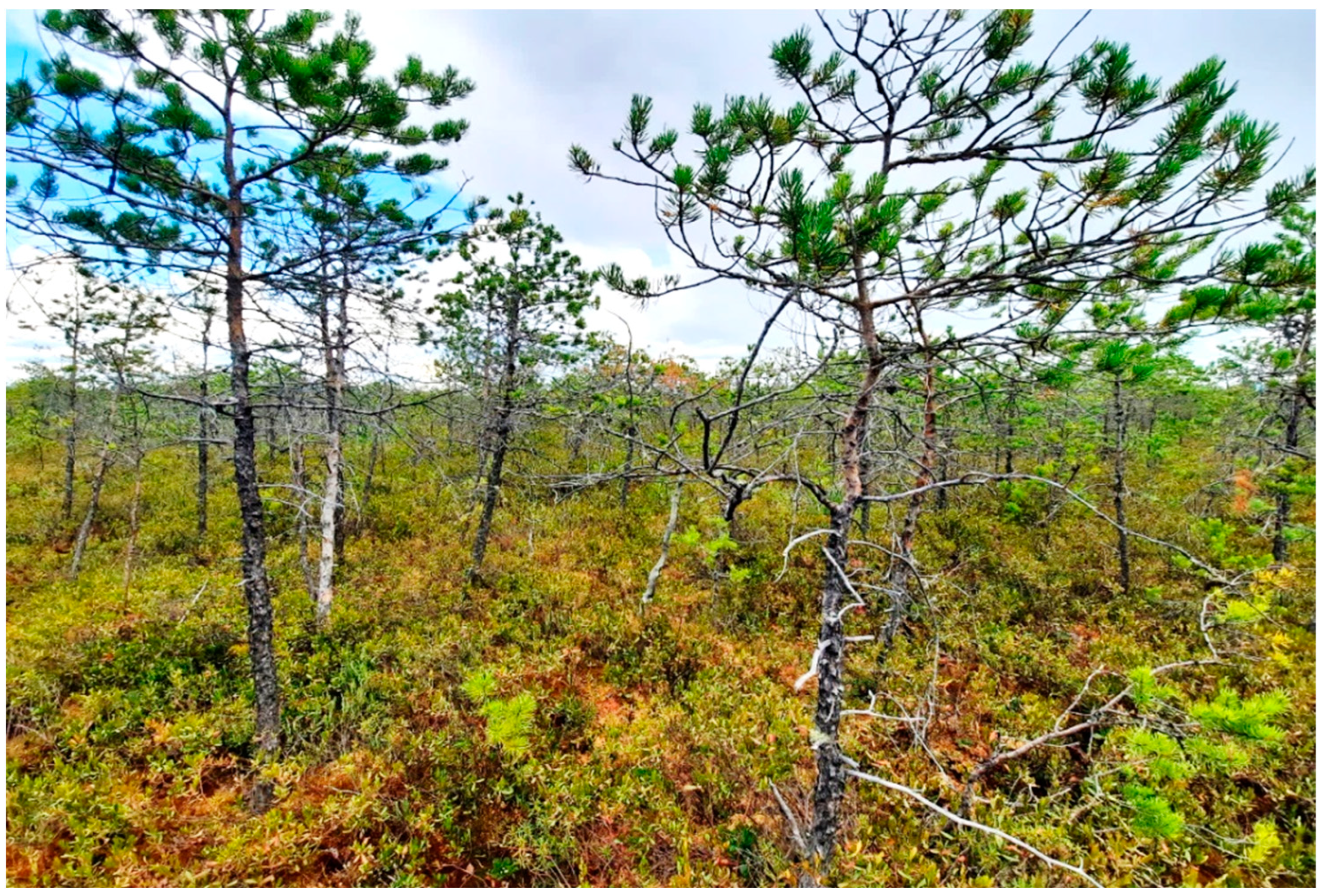
2.1. Study Area

Ground observations were conducted within the northeastern part of the Great Vasyugan Mire in the interfluve of the Bakchar and Iksa Rivers (Figure 1). The Great Vasyugan Mire is the world’s largest mire system with a total area of 55,051 km² [38], which was formed about 10,000 years ago as a result of the coalescence of many small mires [39]. The study was carried out within a pine dwarf shrub-sphagnum vegetation community typical of Western Siberia (56°58′24,3′′; 82°36′41,2′′). The study area is in its natural state and has not been subjected to any anthropogenic impact.

2.2. Sampling Design

CO₂ emissions in the field were measured by the chemical absorption method based on capturing gaseous CO₂ released from the soil surface with NaOH [40] once a month during the vegetation season of 2019, from the 25th of May to the 17th of October. Measurements of the CO₂ flow were duplicated in parallel with a LI-7810SC Li-COR gas analyzer. The comparative measurements of CO₂ emissions by absorption method and by gas analyser [41] showed that the absorption method sizably underestimates (2.5 times) the CO2 flux, which required necessary corrections. Organic matter content in the peat and mineral soil was analyzed on an Agilent 8890 gas chromatograph with an Agilent 5977B mass selective detector and a Frontier Lab EGA/PY-3030D pyrolytic cell, Agilent Technologies. Air temperature (T) and precipitation (P) were obtained from the meteorological station near Bakchar village, according to RIHMI-WDC (http://meteo.ru/ (URL accessed on 1 December 2022). Additionally, data from the T and P sensor system installed directly within the soil profile of the study area was used. Solar radiation was measured directly in the study area of the Great Vasyugan Mire using a BISR solar radiation meter. Temperature data for the peat deposits in the layer up to 1 m were obtained using in situ temperature sensors [42]. The data on the height of snow cover were obtained from ground areal snow measurements in the study area during the period of maximum snow accumulation in March 2019.

The groundwater level (WTL) observations within the GVM were carried out using an autonomous differential pressure sensor [42], installed in a specially designed PVC pipe (piezometer). Measurements of water levels within the GVM were carried out at intervals of 4 h. Peat moisture was determined by weight method. Botanical composition and degree of decomposition were determined by a microscopic method based on plant macrofossil analysis. The density of peat was determined as the ratio of the mass of a dry sample to its volume. For modeling, we also used data on peat moisture content and specific gravity of the GVM [43].

The hydrological conductivity was determined under field conditions over the entire depth of the peat deposit by fixing with the time of filling the sampler of a given volume after pumping water from the borehole. For this purpose, we have arranged a series of boreholes for the entire depth of the peat deposit, via installation of PVC pipes with perforation of 25–50 cm to each specific depth. The Solinst 425 Discrete Sampling System (Solinst Ltd., ON, Canada) and the Solinst 428 sampler were used to conduct the experiment. The redox potential (Eh) of the water was determined with an HM Digital ORP-200 (HM Digital, Inc., Redondo Beach, CA, USA) while the pH value of peat porewater and groundwater was measured with an HM Digital pH-200 (HM Digital, Inc., Redondo Beach, CA, USA).

2.3. Model Wetland-DNDC

Carbon cycle and greenhouse gas emissions/removals from peatlands are governed by closely interacting processes between climate, soil and vegetation under highly variable hydrological conditions. There are several models that allow for the integrating most of the processes occurring in wetland ecosystems [44]. One of the most comprehensive model is Wetland-DNDC [37,45,46], which allows the prediction of CO₂ and CH₄ emissions taking into account hydrological conditions, vegetation growth/decay and biogeochemical processes in wetland ecosystems.

In the Wetland-DNDC model, hydrological conditions, soil temperature, plant growth, soil carbon dynamics, and their processes interact closely. In particular, a hydrological submodel has been developed to assess the dynamics of the groundwater table. The soil profile is divided into layers with different characteristics. The layers are then grouped into two zones: an unsaturated zone above the groundwater table and a saturated zone below. The hydrological submodel takes into account the groundwater table dynamics, surface water inflow (e.g., precipitation, surface inflow, snow/ice melt) and outflow (evaporation, transpiration), as well as water movement within the unsaturated zone. The soil temperature submodel estimates the average daily temperature of each soil layer by numerically solving a one-dimensional (vertical) thermal conductivity equation. The vegetation growth submodel includes mosses, herbaceous plants, and woody vegetation, and it assumes that the total daily plant respiration is proportional to the daily gross photosynthesis of the groundcover vegetation (GPP). Gross photosynthesis is determined by a multiplicative model of maximum photosynthetic rate per unit effective photosynthetic biomass per hour, effective photosynthetic biomass of groundcover vegetation, day length and parameters quantifying the effects of light, temperature and soil moisture, respectively [47]. In the submodel of soil carbon dynamics, soil carbon fluxes and organic matter decomposition processes are controlled by anaerobic processes (CH₄ production and oxidation). For these calculations, the groundwater table or the boundary between anoxic and oxygen-free zone [48] are taken into account, together with available CH₄ production and oxidation rates [49,50]. The redox potential is a direct indicator of the anaerobic state of the soil and is closely related to soil biochemical reactions [51]. Wetland-DNDC uses the redox potential of layers in the saturation zone to simulate anaerobic effects on decomposition, CH₄ formation and oxidation. Model inputs include initial (reservoir) conditions (plant biomass, porosity, soil carbon content, groundwater table depth), water and C flux parameters (lateral inflow/outflow parameters, maximum photosynthetic rate, respiration rate) and climatic factors (daily maximum and minimum temperatures, precipitation, and solar radiation). Many input values can be modified by the user based on actual data from direct field studies. The model outputs include carbon fluxes to the atmosphere, photosynthesis, plant respiration, decomposition of organic matter and net ecosystem productivity. In addition, thermal and hydrological conditions (peat moisture, water table position, peat deposit temperature profile) are taken into account. Calculations of soil C stocks and decomposition processes in the DNDC are provided in detail elsewhere [52,53,54]. To apply the Wetland-DNDC model to peat bogs with a tree layer, recalibration of C decomposition in litter, dead roots and soil waters is required [55,56].

Note the DNDC model used in this study is applicable to any, even very complex, type of wetlands. The pristine area of the GVM site studied in this work is consistent with typical modelling approaches and did not require additional modifications of the mathematical apparatus.

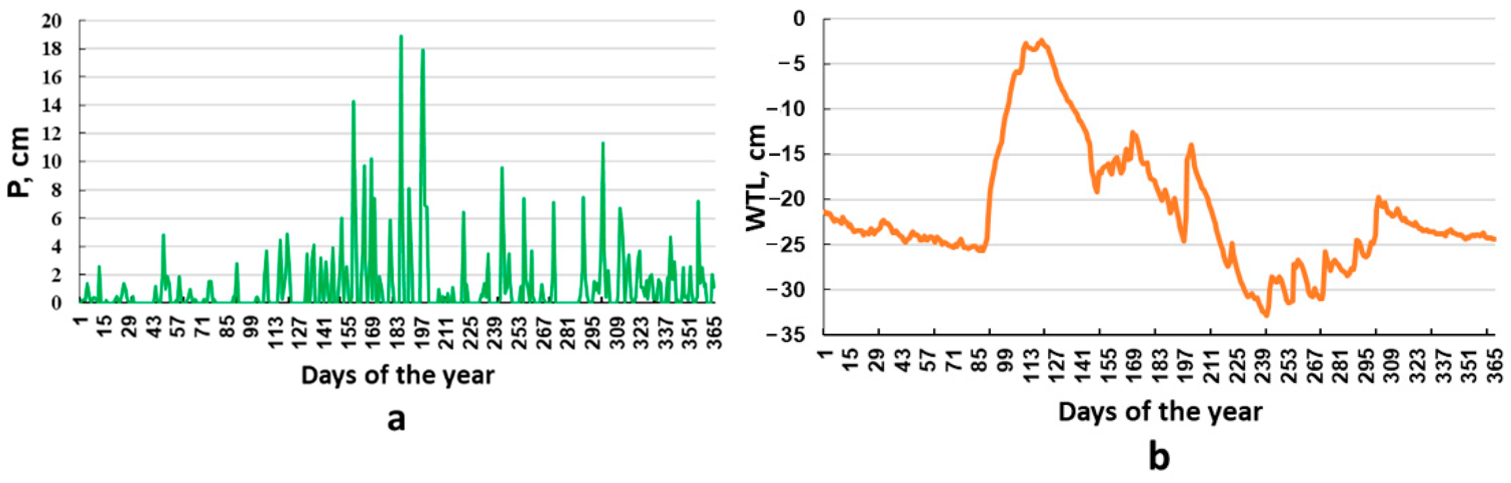
2.4. Climate

The climate of the study area is continental with long cold winters and short hot summers. The average air temperature for the period 1970–2019, according to the Research Institute for Hydrometeorological Information (http://meteo.ru/ (URL accessed on 1 December 2022) is 0.14 °C. In 2020, according to the data from the weather station near Bakchar village, an absolute maximum average annual air temperature of 3.03 °C was recorded. The average annual precipitation for the same period is 485 mm (about 30% falls as snow). The annual amount of precipitation in 2018 was 677 mm, which was the absolute maximum over the years spanning from 1970 to 2020. The average annual hydrological runoff in the nearby Bakchar River is 72 mm [57]. The average precipitation in the period we studied in 2019 was close to the mean perennial annual values and amounted to 431 mm. During 2019, monthly precipitation ranged from 6–15 mm in February and March to 72–89 mm in June–July. The average monthly temperature in February and November 2019 ranged from −18.2 °C to −12.1 °C, rising to 18.1 °C and 16.0 °C in summer (July and August). The average temperature for 2019 was 0.88 °C. The air temperature and solar radiation dynamics used in the model are shown in Figure 2.

Snow cover formed in early November and persisted until mid-April. During this period, a seasonally frozen layer of 13 to 15 cm depth was formed. In 2019, the snow cover height was close to the long-term average, with a maximum snow depth of 74 cm, a peat bog freezing depth of 13 cm. Snowmelt began in early April 2019, and the thawing of the peat deposit began in mid-April. Full thawing of the peat deposit occurred at the end of April.

2.5. Hydrology

The main source of water for the study area of the GVM is atmospheric precipitation. On average, in 2019, the groundwater level was 21 cm below the ground level; the amplitude of annual fluctuations was 31 cm. The groundwater level raised in mid-April due to snowmelt, decreased irregularly in May–June and exhibited a minimum in August. During the springtime, the maximal groundwater levels were observed, exceeding the ground surface in some years. In 2019, the maximum groundwater levels were recorded on 29 April and were 2 cm below the surface of the peat bog. The average summer low water level was 21 cm below the surface, which corresponded to the annual average. The summer low-water period was characterized by a gradual decrease in levels, slightly disturbed by precipitation, until late August, when the lowest level of 33 cm below the bog surface was recorded. In the autumn, from September onwards, there was an increase in level as evaporation decreased, and total precipitation increased (Figure 3a). The maximum rise of the groundwater table to 20 cm below the surface was recorded on 29 October (Figure 3b). During the winter period, there was a gradual decrease in level, which started in November–December and continued until March of the following year due to the lack of atmospheric feeding of the bog. During this period, the snow cover was formed, and the peat deposit of the bog was frozen.

Analysis of multi-year data for the period 2013–2020 shows that in 2018 and 2020, the average annual water levels rise to −18 cm below the surface of the bog, while in 2016, there was a decrease to −25 cm [57].

An important feature of the Western Siberia wetlands is the presence of small lakes inside the mire; in some cases, the lakes can occupy up to 70% of the land surface [21]. Although these small lakes are also an important source of CO₂ and CH₄ fluxes into the atmosphere [58], they were not considered in the present study, which was focused on terrestrial part of C emissions.

2.6. Vegetation

The vegetation of the study area is represented by a pine-shrub-sphagnum plant community (Figure 4). The tree layer is represented by pine, with a protective cover of 40% (crown density 0.4, height up to 2 m, diameter up to 1.5 cm). The grass-bush layer includes Ledum palustre 30%, Chamaedaphne calyculata 60%, Andromeda polifolia 5%, Vaccinium uliginosum 10%, Eriophorum vaginatum 5% and singularly Rubus chamaemorus. Sphagnum mosses stand out (95–100%), of which 80% are represented by S. fuscum, S. balticum, S. divinum and S. angustifolium.

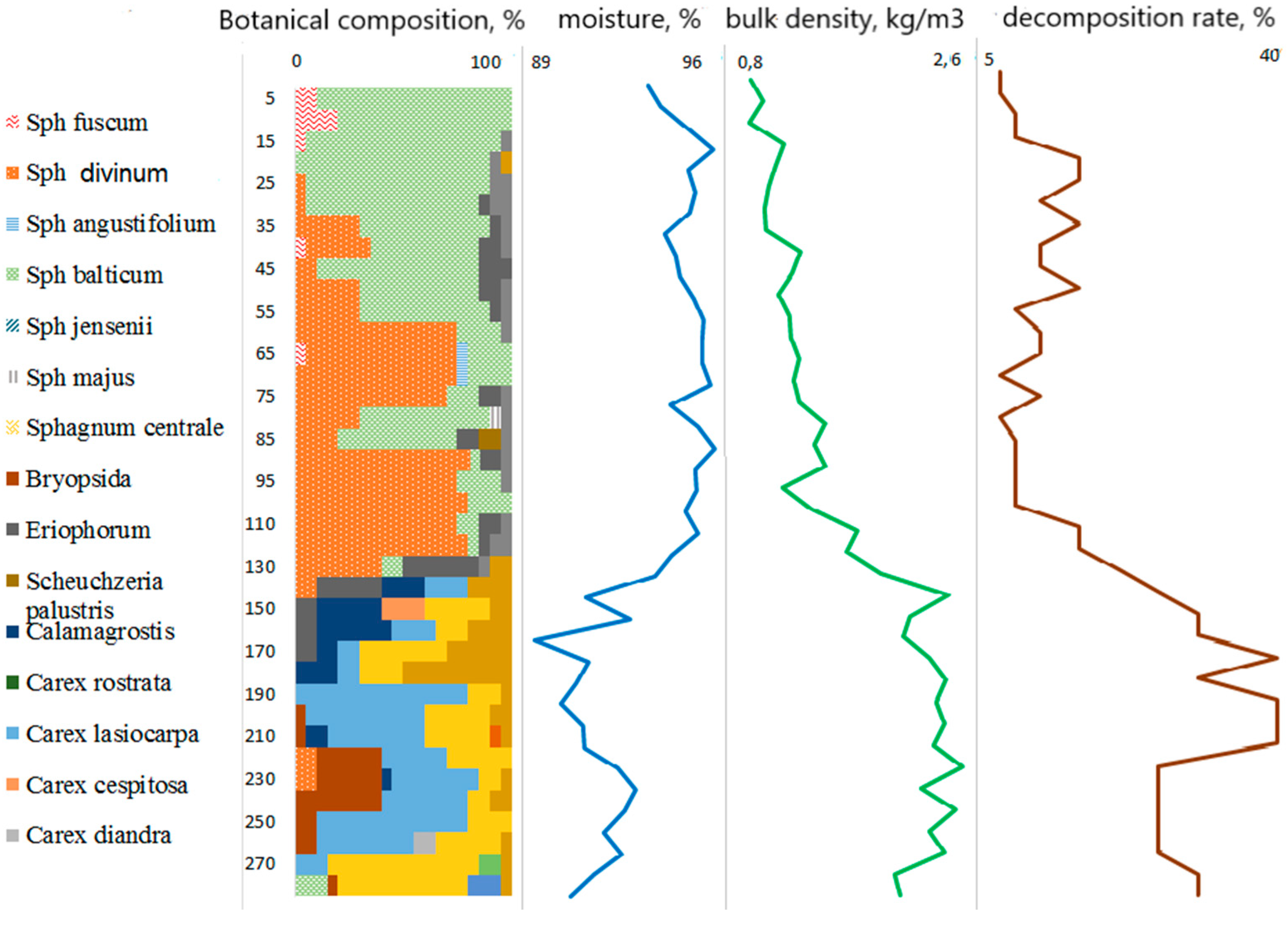
2.7. Peat Deposit

The peat deposit in the study area of GVM is represented by a mixed type. The peat thickness is 285 cm. In the upper part and up to the depth of 120 cm, the peat deposit is composed of Sphagnum peat with a degree of decay 5–15%. Down the profile, it changes to oligotrophic grassy-moss peat, and then to transitional woody-grass peat with a degree of decomposition up to 15%, which increased in the lower part up to 20%. At a depth of 150–285 cm, the peat is composed of eutrophic grassy, woody-grass and grass-moss peat with a degree of decomposition of 20–40%. A more complete description of the peat deposits of the study area is presented elsewhere [57].

2.8. Model Input Values

The input parameters are presented in the Supplementary Materials. The Wetland-DNDC input values were used for each submodel. Daily values of atmospheric temperature (Figure 2a), precipitation (Figure 3a) were retrieved from the meteorological station of the Bakchar village. Values of solar radiation were measured directly at the study site (Figure 2b). Groundwater levels were obtained from borehole measurements (Figure 3b). The vegetation parameters were obtained from field surveys and from published data [41,59,60,61]. Soil parameters were based on the results of field studies (Figure 5). The sequence of data input to the model followed the order climate—hydrology—vegetation—soil.

2.9. Assessment of Modelling Performance

In order to characterize model performance and check for adequacy of applied equations, modelling effectiveness coefficients were used, which allow comparing measured and calculated values between each other.

Determination coefficient or the Nash–Sutcliffe model efficiency coefficient (R²) is described as:

$$R^2=1-\frac{{{\displaystyle \sum }}_i{\left(y_{i-f_i}\right)}^2}{{{\displaystyle \sum }}_i{\left(y_i-\overline{y}\right)}^2}, \overline{y}=\frac{1}{n}{\displaystyle \sum }_{i=1}^n\left(y_i\right)$$

(1)

where $y$_i is observed value, f_i is modelled value. In the best-case scenario, the modelled values coincide with the observed values and R² is equal to 1. The linear least squares multiple regression R² is equal to the square of Pearson’s correlation coefficient between observed and modelled data values of the dependent variable.

The Tale coefficient [62] is calculated according to Equation 2:

$$T=\frac{\sqrt{\frac{1}{N}{{\displaystyle \sum }}_{i=1}^N{\left(X_{real}-X_{model}\right)}^2}}{\sqrt{\frac{1}{N}{{\displaystyle \sum }}_{i=1}^N{\left(X_{real}\right)}^2}+\sqrt{\frac{1}{N}{{\displaystyle \sum }}_{i=1}^N{\left(X_{model}\right)}^2}}$$

(2)

where X_real is the measured value; X_model is the calculated value. The T coefficient ranges from 0 to 1, with most accurate modelling achieved at T = 0. For the modeling of natural processes, a significance threshold of T ≤ 0.3 is usually accepted.

3. Results

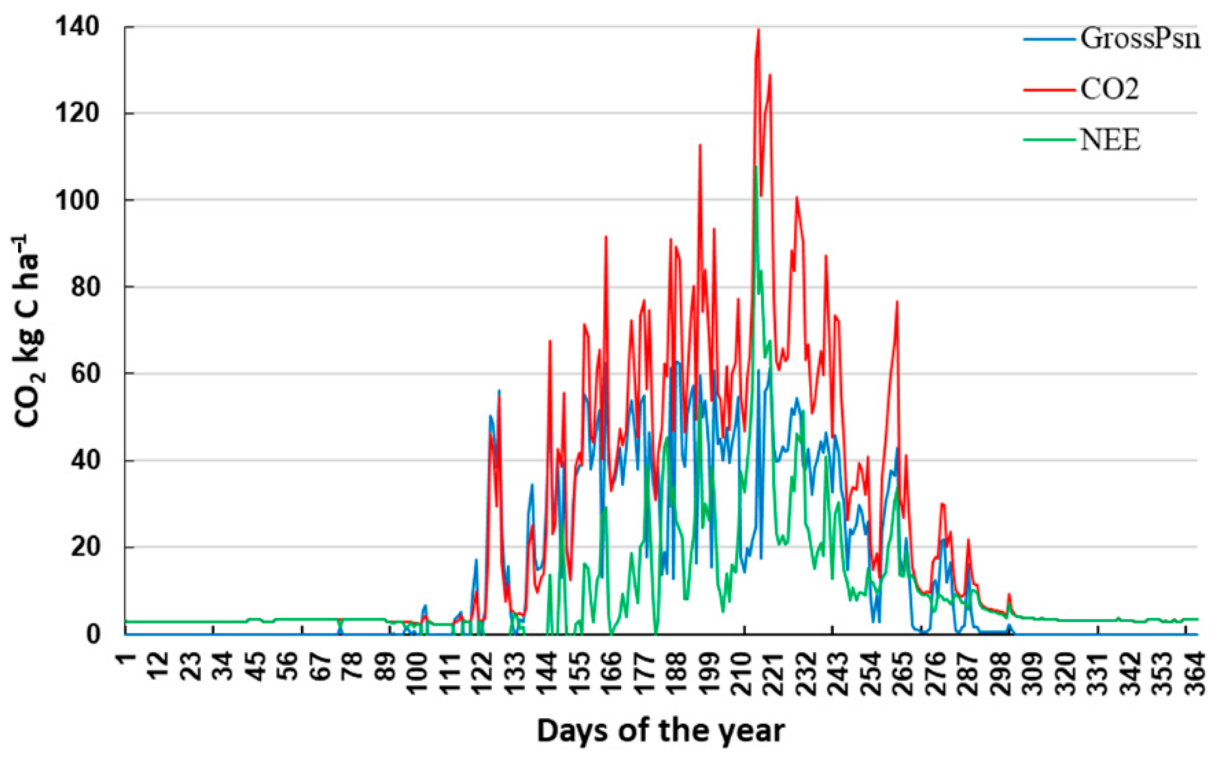
Modelled Outputs

The input parameters of the model are presented in the Supplementary Materials. The model outputs include C and N in mass balances, daily climatic conditions, groundwater level dynamics, carbon and nitrogen storage and fluxes in different compartments of the ecosystem, as well as annual summary of the most important pools and gas fluxes occurring in the ecosystem. The model output is the net ecosystem CO₂ exchange (NEE—net ecosystem exchange). In annual and seasonal output, NEE is net ecosystem production (NEP) or net primary production (NPP), including microbial respiration (RM):

$$-NEE=NEP=NPP-RM$$

(3)

The gross primary production (GPP) equals net primary production plus autotrophic respiration (RA):

$$GPP=NPP+RA or GPP=NEP+RA+RM$$

(4)

where RA + M is ecosystem respiration (autotrophic and soil) with a positive sign indicating the direction of flux from the ecosystem to the atmosphere.

Ecosystem estimates of the carbon balance components RA + RM and GPP are possible based on measurements of the corresponding meteorological indicators. For example, GPP is reconstructed from photosynthetically active radiation (FAR) and RA + RM is approximated from air or soil temperature. Numerous studies demonstrated that the seasonal course of daily CO₂ fluxes depends on weather conditions and follows the dynamics of FAR, air temperature and humidity.

According to the Wetland-DNDC model:

RA + RM = CO₂(plant) + CO₂(litter) + CO₂(soil)

(5)

GPP = GrossPsn and NEE = CO₂ − GrossPsn

(6)

where GrossPsn is the gross photosynthesis of ground vegetation [17].

The simulation results provide detailed, daily information on the distribution of greenhouse gas fluxes throughout the year. In winter, when biological processes are slowed down, the fluxes are minimal. Significant fluctuations in the flux are observed during the growing season. The DNDC model allows testing of the external factors that cause these fluctuations.

Figure 6 shows all calculated CO₂ fluxes for the GVM during 2019. The most significant ecosystem components contributing to the flux calculated via the Wetland-DNDC model on the annual scale are plant-CO₂ (5246 kg C ha⁻¹) and litter-CO₂ (3294 kg C ha⁻¹).

Figure 7 shows model estimates of the fluxes constituting the carbon balance RA + RM = CO₂ and GPP = GrossPsn (NEE = CO₂ − GrossPsn). The net annual NEE value was equal to 3397 kg C ha⁻¹. The calculated fluxes of CH₄ are illustrated in Figure 8.

The total CH₄ flux (net flux) in spring is mainly composed of the CH₄ (diffusion) component and later in the summer–autumn season by the CH₄ (ebullition) component. The calculated fluxes of N components in the course of the year are illustrated in Figure 9. The two most pronounced annual N flux components are NO (9360 g N ha⁻¹ day⁻¹) and N₂O (3726 g N ha⁻¹ day⁻¹).

The results obtained in the simulation are consistent with the structure and functioning of bog ecosystems established in numerous publications that have studied peat bogs of Western Siberia [9,21,22,59,59,61,63].

4. Discussion

Sensitivity Assessment

The simulation results showed that the NEE values and CH₄ emissions are sensitive to most of the tested input variables, while WTL and NPP are sensitive to only a few environmental variables. For example, WTL is primarily influenced by hydrological conditions and climate (precipitation, temperature). NPP is sensitive to the maximum rate of photosynthesis (Amax) but responds weakly to lower temperatures. For NEE, the most important factors are temperature, Amax, plant biomass and soil organic carbon.

Carbon dynamics and CH₄ emissions respond differently to the input factors and are also strongly influenced by interactions between thermal/hydrological conditions, plant growth and soil C dynamics. Therefore, it is critical for the model to integrate hydrology, vegetation, soil and climate when predicting carbon exchange and CH₄ emissions in wetland ecosystems. In work of Taft et al. [64], the effects of different climate and soil input parameters on modelled greenhouse gas fluxes were assessed. These authors demonstrated that the predicted CH₄ flux was only affected by changes in groundwater depth. For a peat bog in the range of parameters tested, adjusting the input values of drainage efficiency, the initial NO₃⁻ concentration at the soil surface, plant vascularization and infiltration rate had no noticeable effect on the modelled GHG emissions. Adjustments for some other parameters (e.g., soil pH, water retention layer depth, initial NH₄ concentration in soil, microbial activity index and N content in water) had little effect on emissions. For more than half of the remaining variables tested in the sensitivity analysis, the GHG emissions showed significant sensitivity to changes in input values. The CO₂ emissions were the most sensitive to soil hydraulic conductivity, soil humus and percentage of persistent litter, humus decomposition rate and maximum biomass production. The N₂O emissions were the most sensitive to the depth of soil organic carbon, forest floor and humus decomposition rates, clay content, porosity and depth of the groundwater table. The sensitivity analysis [52] showed that rainfall patterns strongly influenced N₂O emissions from soils. During the simulated year, changes in temperature, precipitation, organic carbon, clay content and pH had a significant impact on denitrification rates and N₂O emissions.

For the GVM case study, we changed the input parameters of the DNDC model to determine their impact on the result. If the values were unknown, then the input parameters were assigned the mean values of the range. The optimal values of the input parameters of the model were chosen in accordance with the simulation efficiency coefficients.

The input parameters of the "soil" model are presented in the Supplementary Materials. The results of Wetland-DNDC sensitivity analysis to the input parameter “Field capacity” reflecting the moisture content in a peat layer are presented in

Table 1. Modelled annual variants of the Wetland-DNDC sensitivity analysis for input interval parameters of soils.

Parameter	Parameter Values	R2	Σ NEE	Σ CH4
	1 | 2	0.60	2425	258
	0.75 | 2.25	0.67	2452	202
Thickness	0.5 | 2.5	0.67	2502	119
	0.3 | 2.7	0.64	1663	46.5
	0.1 | 2.9	0.59	113	40.0
	0.4	0.67	2476	117
	0.95	0.67	2476	117
Hydrological conductivity	1.5	0.67	2476	117
	2.05	0.67	2476	117
	2.6	0.67	2477	117
	0.46	0.66	1521	118
	0.58	0.66	2127	118
Porosity	0.69	0.67	2502	119
	0.81	0.67	2244	116
	0.92	0.67	2749	117
	0.2	0.67	2749	117
Wilting point	0.45	0.67	2749	117
	0.7	0.67	2749	117
	4 | 30	0.67	2749.4	117
Layers	2 | 15	0.65	1881	46.7
	1 | 15	0.58	81.2	40.6

and Figure 10 and Figure 11.

In Table 1, the “Thickness” is represented by 2 layers: the left value is the thickness of the organic part of the soil, the right one is the thickness of the mineral part (cm). Layers is also represented by 2 layers: the left value is the number of layers of the organic part of the soil, the right one is the mineral part.

They are characterized by almost constant simulation efficiency coefficients (T = 0.86 and R² = 0.59), the weak influence of the “Field capacity” parameter on annual CH₄ flux and a stronger influence on annual NEE flux. The “Field capacity”–NEE relationship could be approximated by a regression function [65], which allowed for the determination of the maximum (optimum) value of Field_max = 0.75.

It is important to note that sensitivity analysis revealed a strong effect of peat volumetric density (in the range 0.10 to 1.38 g cm⁻³) on the GHG fluxes and soil humus leading to occasional failure of the model. GHG emissions of the Wetland-DNDC model (using annual fluxes of NEE and CH₄ fluxes as examples) showed low sensitivity to changes in input values of “Hydrological conductivity“ (R² = 0.67), “Wilting point“ (R² = 0.67) and «Clay organic» (R² = 0.60). NEE and CH₄ emissions were more sensitive to the “Thickness“, “Porosity“ and “Layers“, whose optimum values were determined from the condition of maximum R² and annual NEE.

An analysis of the sensitivity of the Wetland-DNDC model to changes in the range of input parameters revealed insensitivity to sedge or grass layer parameters (R² = 0.52), weak sensitivity to upper-story layer parameters (R² = 0.23) and strong sensitivity to moss layer parameters (R² = −0.63). We therefore focused on the correction of optimal moss layer parameters, among which «Alpha» (range from 0.01 to 0.40) and “Max Psn“ (range from 5.85 to 17.2) were especially interesting (

Table 2. The modelled annual variants of the Wetland-DNDC sensitivity analysis to the moss layer input parameters.

Parameter	Parameter Values	T	R2	Σ NEE	Σ CH4
	0.4	0.11	−0.16	2375	408
	0.2	0.11	−0.10	2389	408
	0.1	0.10	0.00	2415	408
	0.05	0.09	0.18	2459	408
Alpha	0.02	0.08	0.50	2562	408
	0.01	0.07	0.63	2683	408
	0.005	0.11	0.22	2837	408
	0.001	0.34	−4.09	3206	408
	17.2	0.38	−28.0	1414	408
	12	0.28	−10.3	1874	408
	9	0.19	−3.16	2186	408
	6	0.08	0.44	2543	408
Max Psn	5.85	0.08	0.50	2562	408
	5.5	0.07	0.59	2608	408
	5.0	0.07	0.59	2674	408
	3	0.19	−1.11	2959	408
	1	0.42	−6.13	3282	408

). The optimal values of “Alpha“ and “Max Psn“ parameters are determined from the condition of maximum R² (0.63 and 0.59, respectively). Note that, at optimal values of “Alpha“ and “Max Psn“ parameters, the quality of moss layer model increased (R² = 0.41). A similar situation arises in the case of the upper story: “Site fertility class“ (in the range 1.4 to 2.7) with an optimum value of Site opt =1.42857, determined by maximum R² = 0.50 and GHG emission; «Wood» (in the range 6545 to 81102) with optimum Woodopt =60,000 (by maximum R² = 0.57); insensitivity to “Bud C“ (in the range 50 to 950) and “Wood C“ (in the range 1380 to 10,430). Note that with optimal values of the «Site» and “Wood“ parameters, the quality of the model increased (R² = 0.43).

It should be noted that the effectiveness of the Wetland-DNDC simulation model strongly varies across different regions of the world (

Table 3. Effectiveness of the Wetland-DNDC simulation model.

Wetlands	Coefficient of Determination
Wetlands in North America [37]	R2 = 0.52 at N = 468 for groundwater level;
	R2 = 0.91 at N = 59 for soil temperature;
	R2 = 0.76 at N = 214 for CH4 fluxes;
	R2 = 0.49 at N = 266 for NEE ecosystem net productivity
Wetlands in Florida [65]	R2 = 0.71 for groundwater level;
	R2 = 0.62 for CH4 fluxes;
	R2 = 0.75 for NEE
Peat bog in Canada [66]	R2 = 0.79–0.86 for GPP
	R2 = 0.86–0.87 for ecosystem respiration
Wetlands in northeastern and southwestern China, Canada and the USA [67]	R2 = 0.84 for CH4 fluxes
Alpine wetlands in Qinghai–Tibet Plateau [68,69]	R2 = 0.89 for soil temperature;
	R2 = 0.86 for ecosystem respiration;
	R2 = 0.81 for gross primary GPP;
	R2 = 0.52 for NEE ecosystem net productivity
Forest watershed (160 ha) in South Carolina, USA, [70]	R2 = 0.66–0.88, for groundwater level;
	R2 = 0.83 for soil temperature;
	R2 = 0.66 and E = 0.61 for soil CO2 flux

). Nevertheless, the model shows the highest efficiency in all regions (R²) for soil temperature, which largely determines the activity of biochemical processes in plants and soil microorganisms.

In the present case of the test site in the GVM during 2019, for CO₂ (plant + soil), the Tale coefficient was T = 0.085 and the coefficient of determination was R² = 0.675. Therefore, the Wetland-DNDC greenhouse gas emission simulation biogeochemical model adequately reproduced the measured GHG fluxes and demonstrated a sufficient performance in the western Siberian peatlands.

5. Conclusions

The vast Western Siberian wetlands exhibiting a major impact on the global carbon cycle and climate change. However, for assessing the greenhouse gas balance of the area of about 1 million km², it is important to take into account the spatial heterogeneity of landscapes. Direct point measurements of greenhouse gas fluxes in bog ecosystems do not provide sufficient spatial and quantitative coverage for quantifying emissions from a large bog territory. Therefore, a model was used that allows, based on remote sensing data, to estimate greenhouse gas fluxes in different compartments of wetland ecosystems. For this, we chose a typical area of the Great Vasyugan Mire in western Siberia, and we tested the Wetland-DNDC simulation biogeochemical model to calculate greenhouse gas fluxes from the terrestrial ecosystems. We demonstrate adequate efficiency of the model (Nash–Sutcliffe coefficient of 0.675 and Tale coefficient of 0.085), which is comparable with that reported in other wetlands of the world.

An analysis of the sensitivity of the Wetland-DNDC model to the input factors revealed low sensitivity of CO₂ fluxes to the sedge or grass layer, weak sensitivity to the upper tree layer, but high sensitivity to the moss layer. The model is also highly sensitive to the bulk density parameter. Field water capacity has a weak influence on annual CH₄ flux and a stronger influence of on annual NEE. In addition, the low sensitivity of annual NEE and CH₄ fluxes to changes in such input parameters as “Hydroconductivity”, “Wilting Point” and “Clay Organics”. The NEE and CH₄ emissions in the model are more sensitive to changes in the input values of ”Thickness”, “Porosity”, and “Layers”. These results are generally consistent with the structure and functioning of bog ecosystems, as established in previous works on the Western Siberian wetlands.

It is important that the model is well suited to the conditions of bog/mire ecosystems and allows us to consider the impact of hydrothermal factors (temperature, precipitation, groundwater level) on the greenhouse gas fluxes from the land surface. The results obtained make it possible to better define research priorities when collecting primary data in the field. This should allow for further application of this model for the whole western Siberian territory based on remote sensing data.

References

- Yan, L.; Zhang, X.; Wu, H.; Kang, E.; Li, Y.; Wang, J.; Yan, Z.; Zhang, K.; Kang, X. Disproportionate Changes in the CH4 Emissions of Six Water Table Levels in an Alpine Peatland. Atmosphere 2020, 11, 1165. [Google Scholar] [CrossRef]
- Parish, F.; Sirin, A.; Charman, D.; Joosten, H.; Minayeva, T.; Silvius, M.; Stringer, L. (Eds.) Assessment on Peatlands, Biodiversity and Climate Change; Main Report; Global Environment Centre, Kuala Lumpur and Wetlands International: Wageningen, Netherlands, 2008; 179p. [Google Scholar]
- Eswaran, H.E.; Van den Berg, P.R.; Kimble, J. Global soil carbon resources. In Soils and Global Change; Lal, R., Kimble, J., Levine, E., Stewart, B.A., Eds.; CRC Press: Boca Raton, FL, USA, 1995; pp. 27–43. [Google Scholar]
- Harenda, K.M.; Lamentowicz, M.; Samson, M.; Chojnicki, B.H. The Role of Peatlands and Their Carbon Storage Function in the Context of Climate Change. In Interdisciplinary Approaches for Sustainable Development Goals; Springer: Cham, Switzerland, 2017; pp. 169–187. [Google Scholar] [CrossRef]
- Charman, D.J.; Beilman, D.W.; Blaauw, M.; Booth, R.K.; Brewer, S.; Chambers, F.M.; Christen, J.A.; Gallego-Sala, A.; Harrison, S.P.; Hughes, P.D.M.; et al. Climate-related changes in peatland carbon accumulation during the last millennium. Biogeosciences 2013, 10, 929–944. [Google Scholar] [CrossRef] [Green Version]
- Zemtsov, A.A. (Ed.) Bogs of Western Siberia—Their Role in the Biosphere; TSU, SibNIIT: Tomsk, Russia, 1998; 72p. (In Russian) [Google Scholar]
- Resources of Surface Waters of the USSR. Altai and Western Siberia; Middle Ob; Gidrometeoizdat: Leningrad, Russia, 1972; Volume 15, 408p. (In Russian) [Google Scholar]
- Scientific Prerequisites for the Development Bogs of Western Siberia; Nauka: Moscow, Russia, 1977; 247p. (In Russian)
- Liss, O.L.; Berezina, N.A. Bogs of Western Siberia Plain, Moscow; Publishing House of Moscow State University: Moscow, Russia, 1981; 204p. (In Russian) [Google Scholar]
- Kuzmin, G.F. Bogs and Their Use; Sat. Scientific Works VNIIT: Leningrad, Russia, 1993; 139p. (In Russian) [Google Scholar]
- Kosykh, N.P.; Mironycheva-Tokareva, N.P.; Vishnyakova, E.K.; Koronatova, N.G.; Stepanova, V.A.; Kolesnychenko, L.G.; Khovalyg, A.O.; Peregon, A.M. Plant Organic Matter in Palsa and Khasyrei Type Mires: Direct Observations in West Siberian Sub-Arctic. Atmosphere 2021, 12, 1612. [Google Scholar] [CrossRef]
- O’Neill, A.; Tucker, C.; Kane, E.S. Fresh Air for the Mire-Breathing Hypothesis: Sphagnum Moss and Peat Structure Regulate the Response of CO2 Exchange to Altered Hydrology in a Northern Peatland Ecosystem. Water 2022, 14, 3239. [Google Scholar] [CrossRef]
- Li, Y.; Wan, Z.; Sun, L. Simulation of Carbon Exchange from a Permafrost Peatland in the Great Hing’an Mountains Based on CoupModel. Atmosphere 2021, 13, 44. [Google Scholar] [CrossRef]
- Valjarević, A.; Djekić, T.; Stevanović, V.; Ivanović, R.; Jandziković, B. GIS numerical and remote sensing analyses of forest changes in the Toplica region for the period of 1953–2013. Appl. Geogr. 2018, 92, 131–139. [Google Scholar] [CrossRef]
- Poeplau, C.; Schroeder, J.; Gregorich, E.; Kurganova, I. Farmers’ Perspective on Agriculture and Environmental Change in the Circumpolar North of Europe and America. Land 2019, 8, 190. [Google Scholar] [CrossRef] [Green Version]
- Shurpali, N.; Verma, S.B.; Kim, J.; Arkebauer, T.J. Carbon dioxide exchange in a peatland ecosystem. J. Geophys. Res. Earth Surf. 1995, 100, 14319–14326. [Google Scholar] [CrossRef]
- Silvola, J.J.; Alm, J.; Ahlholm, U.; Nykanen., H.; Martikainen, P.J. CO2 fluxes from peat in boreal mires under varying tem-perature and moisture conditions. J. Ecol. 1996, 84, 219–228. [Google Scholar] [CrossRef]
- Bubier, J.L.; Crill, P.M.; Moore, T.R.; Savage, K.; Varner, R.K. Seasonal patterns of controls on net ecosystem CO2 exchange in a boreal peatland complex. Global Biogeochem. Cycles 1998, 12, 703–714. [Google Scholar] [CrossRef] [Green Version]
- Berezin, A.E.; Bazanov, V.A.; Parshina, N.V. The influence of the oil and gas complex on the bogs of the Western Siberia taiga zone. Int. J. Environ. Stud. 2014, 71, 716–721. [Google Scholar] [CrossRef]
- Shevchenko, V.; Vorobyev, S.; Krickov, I.; Boev, A.; Lim, A.; Novigatsky, A.; Starodymova, D.; Pokrovsky, O. Insoluble Particles in the Snowpack of the Ob River Basin (Western Siberia) a 2800 km Submeridional Profile. Atmosphere 2020, 11, 1184. [Google Scholar] [CrossRef]
- Vasyugan Mire (Natural Conditions, Structure and Functioning); Inisheva, L.I. (Ed.) TSNTI: Tomsk, Russia, 2000; 181p. (In Russian) [Google Scholar]
- Bernatonis, V.K.; Arkhipov, V.S.; Zdvizhkov, M.A.; Preis Yu, I.; Tikhomirov, N.O. Geochemistry of plants and peat of the Great Vasyugan mire. In Great Vasyugan Mire. Current State and Development Processes; Publishing House of the Siberian Branch of the Russian Academy of Sciences: Tomsk, Russia, 2002; pp. 204–215. (In Russian) [Google Scholar]
- Kabanov, M.V. (Ed.) Study of Natural and Climatic Processes on the Territory of the Great Vasyugan Mire; Publishing House of the Siberian Branch of the Russian Academy of Sciences: Novosibirsk, Russia, 2012; 243p. (In Russian) [Google Scholar]
- Berezin, A.E.; Bazanov, V.A.; Skugarev, A.A.; Rybina, T.A.; Parshina, N.V. Landscapes of the Great Vasyugan Mire. In Peatlands of Western Siberia and the Carbon Cycle: Past and Present, Proceedings of the Fourth International Field Symposium, Novosibirsk; Tomsk, Russia, 4–17 August 2014, Publishing House: TSU, Tomsk, Russia, 2014; pp. 50–52. Available online: http://vital.lib.tsu.ru/vital/access/manager/Repository/vtls:000509240 (accessed on 10 October 2022).
- Cade, S.M.; Clemitshaw, K.C.; Molina-Herrera, S.; Grote, R.; Haas, E.; Wilkinson, M.; Morison, J.I.L.; Yamulki, S. Evaluation of LandscapeDNDC Model Predictions of CO2 and N2O Fluxes from an Oak Forest in SE England. Forests 2021, 12, 1517. [Google Scholar] [CrossRef]
- Li, C. Quantifying greenhouse gas emissions from soils: Scientific basis and modeling approach. Soil Sci. Plant Nutr. 2007, 53, 344–352. [Google Scholar] [CrossRef] [Green Version]
- Giltrap, D.L.; Li, C.; Saggar, S. DNDC: A process-based model of greenhouse gas fluxes from agricultural soils. Agric. Ecosyst. Environ. 2010, 136, 292–300. [Google Scholar] [CrossRef]
- Peltoniemi, M.; Thürig, E.; Ogle, S.; Palosuo, T.; Schrumpf, M.; Wutzler, T.; Butterbach-Bahl, K.; Chertov, O.; Komarov, A.; Mikhailov, A.; et al. Models in country scale carbon accounting of forest soils. Silva Fenn. 2007, 41, 575–602. [Google Scholar] [CrossRef] [Green Version]
- Bell, M.J.; Jones, E.; Smith, J.; Smith, P.; Yeluripati, J.; Augustin, J.; Juszczak, R.; Olejnik, J.; Sommer, M. Simulation of soil nitrogen, nitrous oxide emissions and mitigation scenarios at 3 European cropland sites using the ECOSSE model. Nutr. Cycl. Agroecosystems 2011, 92, 161–181. [Google Scholar] [CrossRef]
- Cigno, E.; Magagnoli, C.; Pierce, M.; Iglesias, P. Lubricating ability of two phosphonium-based ionic liquids as additives of a bio-oil for use in wind turbines gearboxes. Wear 2017, 376–377, 756–765. [Google Scholar] [CrossRef]
- Deng, J.; Li, C.; Frolking, S. Modeling impacts of changes in temperature and water table on C gas fluxes in an Alaskan peatland. J. Geophys. Res. Biogeosci. 2015, 120, 1279–1295. [Google Scholar] [CrossRef]
- Sukhoveeva, O.E. Parameterization of the dndc model for assessing the components of the biogeochemical carbon cycle in European Russia. Bull. St. Petersburg State Univ. Earth Sci. 2019, 64, 363–384. [Google Scholar] [CrossRef] [Green Version]
- Janse, J.H.; van Dam, A.A.; Hes, E.M.; de Klein, J.J.; Finlayson, C.M.; Janssen, A.B.; van Wijk, D.; Mooij, W.; Verhoeven, J.T. Towards a global model for wetlands ecosystem services. Curr. Opin. Environ. Sustain. 2018, 36, 11–19. [Google Scholar] [CrossRef]
- Golovatskaya, E.A.; Dyukarev, E.A. The influence of environmental factors on the CO2 emission from the surface of oligotrophic peat soils in West Siberia. Eurasian Soil Sci. 2012, 45, 588–597. [Google Scholar] [CrossRef]
- Dyukarev, E.; Zarov, E.; Alekseychik, P.; Nijp, J.; Filippova, N.; Mammarella, I.; Filippov, I.; Bleuten, W.; Khoroshavin, V.; Ganasevich, G.; et al. The Multiscale Monitoring of Peatland Ecosystem Carbon Cycling in the Middle Taiga Zone of Western Siberia: The Mukhrino Bog Case Study. Land 2021, 10, 824. [Google Scholar] [CrossRef]
- Inisheva, L.I.; Golovchenko, A.V. Monitoring of Greenhouse Gas Production on the Landscape Profile of the Vasyugan Swamp. Eurasian Soil Sci. 2022, 55, 1222–1234. [Google Scholar] [CrossRef]
- Zhang, Y.; Li, C.; Trettin, C.C.; Li, H.; Sun, G. An integrated model of soil, hydrology, and vegetation for carbon dynamics in wetland ecosystems. Glob. Biogeochem. Cycles 2002, 16, 9-1–9-17. [Google Scholar] [CrossRef] [Green Version]
- Berezin, A.; Bazanov, V.; Skugarev, A.; Rybina, T.; Parshina, N. Great Vasyugan Mire: Landscape structure and peat deposit structure features. Int. J. Environ. Stud. 2014, 71, 618–623. [Google Scholar] [CrossRef]
- Kirpotin, S.N.; Antoshkina, O.A.; Berezin, A.E.; Elshehawi, S.; Feurdean, A.; Lapshina, E.D.; Pokrovsky, O.S.; Peregon, A.M.; Semenova, N.M.; Tanneberger, F.; et al. Great Vasyugan Mire: How the world’s largest peatland helps addressing the world’s largest problems. Ambio 2021, 50, 2038–2049. [Google Scholar] [CrossRef]
- Makarov, B.N. A simplified method for determining soil respiration (biochemical activity). Soil Sci. 1957, 9, 119–122. [Google Scholar]
- Golovatskaya, E.A.; Dyukarev, E.A. Seasonal and diurnal dynamics of CO2 emission from oligotrophic peat soil surface. Russ. Meteorol. Hydrol. 2011, 36, 413–419. [Google Scholar] [CrossRef]
- Bazarov, A.V.; Badmaev, N.B.; Kurakov, S.A.; Gonchikov, B.-M.N. Erratum to: A Mobile Measurement System for the Coupled Monitoring of Atmospheric and Soil Parameters. Russ. Meteorol. Hydrol. 2018, 43, 795–796. [Google Scholar] [CrossRef]
- Sinyutkina, A. Drainage consequences and self-restoration of drained raised bogs in the south-eastern part of Western Siberia: Peat accumulation and vegetation dynamics. Catena 2021, 205, 105464. [Google Scholar] [CrossRef]
- Mitsch, W.J.; Sraskraba, M.; Jorgensen, S.E. (Eds.) Wetland Modeling: Development in Environmental Modeling; Elsevier Science: New York, NY, USA, 1988; Volume 12, p. 227. [Google Scholar]
- User’s Guide for Wetland-DNDC. Available online: https://www.dndc.sr.unh.edu/model/ForestUserGuide.pdf (accessed on 10 October 2022).
- Kurbatova, J.; Li, C.; Tatarinov, F.; Varlagin, A.; Shalukhina, N.; Olchev, A. Modeling of the carbon dioxide fluxes in European Russia peat bogs. Environ. Res. Lett. 2009, 4, 045022. [Google Scholar] [CrossRef]
- Frolking, S.; Goulden, M.; Wofsy, S.; Fan, S.-M.; Sutton, D.; Munger, J.; Bazzaz, A.M.; Daube, B.; Crill, P.M.; Aber, J.D.; et al. Modelling temporal variability in the carbon balance of a spruce/moss boreal forest. Glob. Chang. Biol. 1996, 2, 343–366. [Google Scholar] [CrossRef] [Green Version]
- Walter, B.P.; Heimann, M. A process-based, climate-sensitive model to derive methane emissions from natural wetlands: Application to five wetland sites, sensitivity to model parameters, and climate. Glob. Biogeochem. Cycles 2000, 14, 745–765. [Google Scholar] [CrossRef] [Green Version]
- Cao, M.; Marshall, S.; Gregson, K. Global carbon exchange and methane emissions from natural wetlands: Application of a process-based model. J. Geophys. Res. 1996, 101, 399–414. [Google Scholar] [CrossRef] [Green Version]
- Potter, C.S. An ecosystem simulation model for methane production and emission from wetlands. Glob. Biogeochem. Cycles 1997, 11, 495–506. [Google Scholar] [CrossRef]
- Fiedler, S.; Sommer, M. Methane emissions. ground water levels and redox potentials of common wetland soils in a temper-ate-humid climate. Glob. Biogeochem. Cycles 2000, 14, 1081–1093. [Google Scholar] [CrossRef]
- Li, C.; Frolking, S.; Frolking, T.A. A model of nitrous oxide evolution from soil driven by rainfall events: 1. Model structure and sensitivity. J. Geophys. Res. Atmos. 1992, 97, 9759–9776. [Google Scholar] [CrossRef]
- Li, C.; Aber, J.; Stange, F.; Butterbach-Bahl, K.; Papen, H. A process-oriented model of N2O and NO emissions from forest soils: 1. Model development. J. Geophys. Res. 2000, 105, 4369–4384. [Google Scholar] [CrossRef]
- Li, C.S. Modeling Trace Gas Emissions from Agricultural Ecosystems. Nutr. Cycl. Agroecosyst. 2000, 58, 259–276. [Google Scholar] [CrossRef]
- Gilhespy, S.L.; Anthony, S.; Cardenas, L.; Chadwick, D.; del Prado, A.; Li, C.; Misselbrook, T.; Rees, R.M.; Salas, W.; Sanz-Cobena, A.; et al. First 20 years of DNDC (DeNitrification DeComposition): Model evolution. Ecol. Model. 2014, 292, 51–62. [Google Scholar] [CrossRef] [Green Version]
- Kharanzhevskaya, Y.A.; Sinyutkina, A.A. Investigating the role of bogs in the streamflow formation within the Middle Ob Basin. Geogr. Nat. Resour. 2017, 38, 256–266. [Google Scholar] [CrossRef]
- Kharanzhevskaya, Y.; Maloletko, A.; Sinyutkina, A.; Giełczewski, M.; Kirschey, T.; Michałowski, R.; Mirosław-Świątek, D.; Okruszko, T.; Osuch, P.; Trandziuk, P.; et al. Assessing mire-river interaction in a pristine Siberian bog-dominated watershe—Case study of a part of the Great Vasyugan Mire, Russia. J. Hydrol. 2020, 590, 125315. [Google Scholar] [CrossRef]
- Karlsson, J.; Serikova, S.; Vorobyev, S.N.; Rocher-Ros, G.; Denfeld, B.; Pokrovsky, O.S. Carbon emission from Western Siberian inland waters. Nat. Commun. 2021, 12, 825. [Google Scholar] [CrossRef]
- Dyukarev, E.A. Modeling of seasonal carbon exchange in bog ecosystems. Ecology. Economy. Informatics. Syst. Anal. Model. Econ. Ecol. Syst. 2020, 1, 56–61. [Google Scholar] [CrossRef]
- Koronatova, N.G.; Kosykh, N.P. Productivity of the tree layer in raised bogs in the taiga zone of Western Siberia. Forestry 2022, 4, 432–448. [Google Scholar]
- Koronatova, N.; Institute of Soil Science and Agrochemistry of the Siberian Branch of the Russian Academy of Sciences. Review of studies of production and destruction processes in the mires of West Siberia: Methods and results. Soils Environ. 2022, 5. [Google Scholar] [CrossRef]
- Tale, G. Economic Forecasting and Decision Making; Statistician: Moscow, Russia, 1977; 282p. [Google Scholar]
- Savicheva, O.G.; Inisheva, L.I. Biochemical activity of the peat soil of a river marsh ecosystem. Contemp. Probl. Ecol. 2008, 1, 666–672. [Google Scholar] [CrossRef]
- Taft, H.E.; Cross, P.A.; Hastings, A.; Yeluripati, J.; Jones, D.L. Estimating greenhouse gases emissions from horticultural peat soils using a DNDC modelling approach. J. Environ. Manag. 2019, 233, 681–694. [Google Scholar] [CrossRef]
- Cui, J.; Li, C.; Sun, G.; Trettin, C. Linkage of MIKE SHE to Wetland-DNDC for carbon budgeting and anaerobic biogeochemistry simulation. Biogeochemistry 2005, 72, 147–167. [Google Scholar] [CrossRef]
- Kim, Y.; Roulet, N.T.; Peng, C.; Li, C.; Frolking, S.; Strachan, I.B.; Tremblay, A. Multi-year carbon dioxide flux simulations for mature canadian black spruce forests and ombrotrophic bogs using forest-dndc. Boreal Environ. Res. 2014, 19, 417–440. [Google Scholar]
- Li, T.; Huang, Y.W.; Zhang, S.C. CH4 MODwetland: A biogeophysical model for simulating methane emissions from natural wetlands. Ecol. Model. 2010, 221, 666–680. [Google Scholar] [CrossRef]
- Kang, X.; Li, Y.; Wang, J.; Yan, L.; Zhang, X.; Wu, H.; Yan, Z.; Zhang, K.; Hao, Y. Precipitation and temperature regulate the carbon allocation process in alpine wetlands: Quantitative simulation. J. Soils Sediments 2020, 20, 3300–3315. [Google Scholar] [CrossRef]
- Song, C.; Luo, F.; Zhang, L.; Yi, L.; Wang, C.; Yang, Y.; Li, J.; Chen, K.; Wang, W.; Li, Y.; et al. Nongrowing Season CO2 Emissions Determine the Distinct Carbon Budgets of Two Alpine Wetlands on the Northeastern Qinghai—Tibet Plateau. Atmosphere 2021, 12, 1695. [Google Scholar] [CrossRef]
- Dai, Z.; Trettin, C.C.; Li, C.; Li, H.; Sun, G.; Amatya, D.M. Effect of Assessment Scale on Spatial and Temporal Variations in CH4, CO2, and N2O Fluxes in a Forested Wetland. Water Air Soil Pollut. 2011, 223, 253–265. [Google Scholar] [CrossRef]