Article

Evaluation of Empirical Atmospheric Models Using Swarm-C Satellite Data

1
Department of Geography and Anthropology, Louisiana State University, Baton Rouge, LA 70803, USA
2
School of Automation, University of Electronic Science and Technology of China, Chengdu 610054, China
*
Author to whom correspondence should be addressed.
Atmosphere 2022, 13(2), 294; https://doi.org/10.3390/atmos13020294
Submission received: 1 December 2021 / Revised: 5 February 2022 / Accepted: 5 February 2022 / Published: 9 February 2022
(This article belongs to the Special Issue Ionospheric Monitoring and Modelling for Space Weather)

Abstract

:
Swarm-C satellite, a new instrument for atmospheric study, has been the focus of many studies to evaluate its usage and accuracy. This paper takes the Swarm-C satellite as a research object to verify the Swarm-C accelerometer’s inversion results. This paper uses the two-row orbital elements density inversion to verify the atmospheric density accuracy results of the Swarm-C satellite accelerometer. After the accuracy of the satellite data is verified, this paper conducts comparative verification and empirical atmospheric model evaluation experiments based on the Swarm-C accelerometer’s inversion results. After comparing with the inversion results of the Swarm-C semi-major axis attenuation method, it is found that the atmospheric density obtained by inversion using the Swarm-C accelerometer is more dynamic and real-time. It shows that with more available data, the Swarm-C satellite could be a new high-quality instrument for related studies along with the well-established satellites. After evaluating the performance of the JB2008 and NRLMSISE-00 empirical atmospheric models using the Swarm-C accelerometer inversion results, it is found that the accuracy and real-time performance of the JB2008 model at the altitude where the Swarm-C satellite is located are better than the NRLMSISE-00 model.

1. Introduction

It is crucial to study the atmospheric density of the thermosphere. The atmospheric density of the thermosphere can be applied to a variety of different scientific researches and different types of satellite orbit calculations. Its application scope includes satellite return prediction, space object orbit maneuver planning and maintenance, and the thruster’s fuel carrying capacity estimation. The thermosphere’s atmospheric density is one of the most critical research objects in geophysics [1,2,3]. It is also one of the critical variables for calculating drag in satellite precise orbit determination.
The improvement of the observational data of thermosphere atmospheric density and the horizontal wind has promoted various atmospheric models [4,5]. The existing atmospheric models are mainly physical and empirical [6,7,8]. These two types of models have their advantages and application areas. The physical model is based on fundamental physical functions. This series includes the global atmospheric circulation model (TGCM) and local high-resolution airflow models [9,10]. These models can simulate the temperature, density, composition, horizontal wind, and atmosphere’s response to different energy inputs. The empirical model consists of several sets of relatively simple functions, usually used to represent long-term and large-scale atmospheric characteristic changes [11,12,13]. These functions contain parameters fitted using existing observation data. A large amount of observation data is needed to improve the model’s accuracy. The prediction accuracy of the existing atmospheric models, whether physical or empirical, depends on the solar activity cycle and geomagnetic activity index’s prediction accuracy.
The main empirical models are the Jacchia series model, the Drag Temperature Model (DTM) series model, and the Mass Spectrometer Incoherent Scatter (MSIS) series model [14]. These empirical atmospheric models have been widely used in modern satellite orbit determination. Jacchia and MSIS series atmospheric models are more frequently used than DTM series models. However, the Jacchia, MSIS, and DTM series models rely too much on the correlation between atmospheric density, temperature, composition, and F10.7, AP, and KP indices. During the quiet period of geomagnetic activity, the atmospheric density error predicted by these complex empirical atmospheric models at an altitude of about 300 km is about 20%. For extreme atmospheric conditions, the correlation between these variables will become smaller. Therefore, in extreme atmospheric conditions, the empirical atmospheric model’s accuracy is sometimes even reduced to 15%, depending on the geomagnetic activity level at that time [15]. It is worth noting that although the empirical atmospheric model has been developed in the past 20 years, its accuracy has not been significantly improved. It is impossible to fully capture the upper atmosphere’s variation regulation in extreme cases using a set of solar activity cycle variables and geomagnetic activity levels. It is also impossible to predict extreme cases’ atmospheric parameters through the past observation data [16]. Due to these limitations of the empirical model, there is no breakthrough in estimating atmospheric density and improving the empirical model’s accuracy. Therefore, atmospheric density at high spatial and temporal resolution is essential for evaluating and improving the existing atmospheric density model [17].
In the 1950s, human beings first studied the atmospheric reverse resistance of satellites in space, which paved the way for the classic atmospheric models that followed in the 1960s and early 1970s [18,19,20]. These classical atmospheric models include the MSIS series model, the Priester series model, and the Jacchia series model. The Jacchia-71 model was used as a COSPAR international reference atmosphere in 1972, called Cira-72. Jacchia 70 and Jacchia-71 models have been used as the basis of the NASA Marshall engineering thermosphere (MET). In addition, these models have been applied to satellite life prediction. However, it is a pity that Jacchia’s late model accuracy has not been greatly improved.
From the late 1970s, Alan Hedin and others created a new density model called MSIS, based entirely on the mass spectrometer and incoherent scattering radar observations. The MSIS-86 atmospheric model replaced the Jacchia-71 atmospheric model as the COSPAR international reference atmospheric model, called CIRA-86. Subsequently, the model was expanded and developed into the MSISE-90 atmospheric model. In 2000, Picone and other Navy Research Laboratory (NRL) researchers proposed the NRLMSISE-00 atmospheric model [21]. This model is an improvement on the MSISE-90 atmospheric model. MSIS indicates that the mass spectrometer incoherent scattering radar obtains the atmospheric composition of the atmospheric model. The atmospheric model also contains the thermosphere atmosphere and covers the dissipative bottom layer, covering an altitude range of about 0–1000 km.
The main purpose of this paper is as follows:
(1)
Verify the atmospheric density obtained by the Swarm-C accelerometer inversion and use the atmospheric density obtained by the two-line orbital element method to verify the accuracy of the accelerometer inversion result;
(2)
The accelerometer’s density result and result from the two-line orbital number inversion were compared to discuss the accelerometer inversion of atmospheric density;
(3)
The accelerometer inversion results were used to evaluate the NRLMSISE-00 and JB2008 empirical atmosphere models. The accuracy and real-time performance of the two empirical atmosphere models were compared.

2. Data Acquisition and Processing

The Swarm series by the European Space Agency (ESA) began to launch on 22 November 2013 and carry satellite-borne accelerometers and GPS receivers as part of their scientific payload [22,23]. GPS receivers provide position and time-related information for magnetic field measurement. They can be used to determine non-conservative forces, such as the atmospheric reverse resistance and solar radiation pressure acting on the spacecraft. The accelerometer can directly measure these forces [22]. The measurement result is much higher than the resolution of the GPS receiver. In addition, the thermosphere atmospheric density can be extracted from the Swarm satellite accelerometer.
The data used in this article are from:
Swarm satellite data: https://earth.esa.int/eogateway/missions/swarm accessed on 7 December 2018.
The satellites Swarm A, B, and C suffer from different disturbances. The Swarm-A acceleration data has more disturbances than Swarm-B and C. Swarm-B has a lower signal-to-noise ratio than A and C. Therefore, Swarm-C was chosen to be the research target in this paper. We chose the Level-2 product produced by ESA. The acceleration data need to be calibrated before use. Equation (1) used to calibrate the data is:
a c a l ( t ) = s ( t ) ( a r a w ( t ) + b s ( t ) ) a g g ( t ) a c a ( t ) + b T ( t ) + b ( t )
In the equation above, t is the epoch, a c a l is the acceleration after calibration, s ( t ) is the scale factor, b s ( t ) is the step correction, a g g ( t ) is the acceleration caused by gravity, a c a ( t ) is the centrifugal acceleration, b T ( t ) is bias related to temperature variations, b ( t ) is a bias that has no relationship with temperature. The main disturbance in Swarm-C is steps, EDAC failure events, bias caused by temperature changes, and acceleration spikes caused by thruster activation. Data in Figure 1 is from Swarm X-axis accelerometer records on 1 January 2016. The raw data and the calibrated data are shown below.

3. Methods

3.1. Conversion of Orbital Coordinates and Time

The precise orbit data of the Swarm-C satellite contains real-time position coordinates and real-time speed coordinates. The position coordinates and velocity coordinates are in the ITRF geo-fixed system coordinates [24]. In order to study the movement of a satellite, the data in its precise orbit needs to be transferred to the J2000 coordinate system. The specific conversion method is as follows [25].
The satellite’s coordinate in the J2000 coordinate system is r = ( r x , r y , r z ) , and the coordinate value r can be obtained by Equation (2):
r = ( x E c o s θ + y E s i n θ x E s i n θ + y E c o s θ z E )
Suppose the velocity coordinate under J2000 is r = ( r x , r y , r z ) . Taking the derivation on both sides of the above formula separately, the velocity coordinate V under J2000 can be obtained as shown in Equation (3):
v = ( x E θ ˙ s i n θ + v E x c o s θ + y E θ ˙ c o s θ + v E y s i n θ x E θ ˙ c o s θ v E s i n θ y E θ ˙ s i n θ + v E y c o s θ v E z ) .

3.2. Calculation of Satellite Anti-Ballistic Coefficient

The calculation method of anti-ballistic coefficient B is shown in Equation (4). In the formula, C D is the damping coefficient of the satellite, A is the effective area of the satellite, and m is the satellite’s mass [26,27]:
B = C D A m
In density inversion based on accelerometer data, the most important thing is to estimate the parameter accurately C D . ESA gives the areas and normal vectors of each panel of Swarm. The first step is to calculate the drag force on each satellite panel and then sum it up. The resistance coefficient is calculated based on the Sentman function [28]. Define u D as the unit vector of resistance. Then it can be expressed as Equation (5):
u D = v r | v r |
In the function, v r is the velocity of the satellite towards the atmosphere. Define u N as the unit normal vector of the satellite’s panel, define γ as the cosine of the angle between molecular flow and the normal vector of the satellite’s panel. Then, γ is calculated using Equation (6):
γ   = u D u N
Then the molecular speed ratio S can be calculated using Equation (7):
S = | v r | 3 R T m a
In Equation (7), m a is the molar mass of the gas.
The kinetic temperature T i n of the incident gas can be calculated using Equation (8) [29]:
T i n = m a v r 2 3 R
The gas-particle velocity v o u t after collision can be expressed by Equation (9):
v o u t = v r 2 3 [ 1 + a E ( T w a l l T i n 1 ) ]
T i n is the temperature of the incident airflow. v o u t is the speed of the emergent airflow. T w a l l is the temperature of the satellite’s panel. a E is a constant.
Therefore, for the k -th panel of the satellite, the product formula of the atmospheric damping coefficient and the effective area of the panel is as shown in Equation (10):
C D k A k = ( P π + γ k Q Z + γ 2 v o u t v r ( γ k π Z + P ) ) A k
In Equation (10), G = 1 2 S 2 , P = 1 S e x p ( γ 2 S 2 ) , Q = 1 + G , Z = 1 + e r f ( γ S ) .
The atmospheric density ρ around the final satellite orbit can be calculated using Equation (11):
ρ = a c a l ( 1 2 C D A m v r 2 )                    

4. Results

4.1. Verification of Accelerometer Results from Swarm-C Satellite Orbit Data Inversion

This section will use the two-row orbital elements [30] of the Swarm-C satellite to perform atmospheric density inversion and use the inversion results of the two-row orbital elements to verify the atmospheric density accuracy results of the Swarm-C satellite accelerometer. The semi-major axis attenuation method retrieves the atmospheric density based on the Swarm-C satellite’s precise orbit data. Then, the atmospheric density results obtained using the semi-major axis attenuation method [31] are compared and verified with the Swarm-C satellite accelerometer’s atmospheric density.
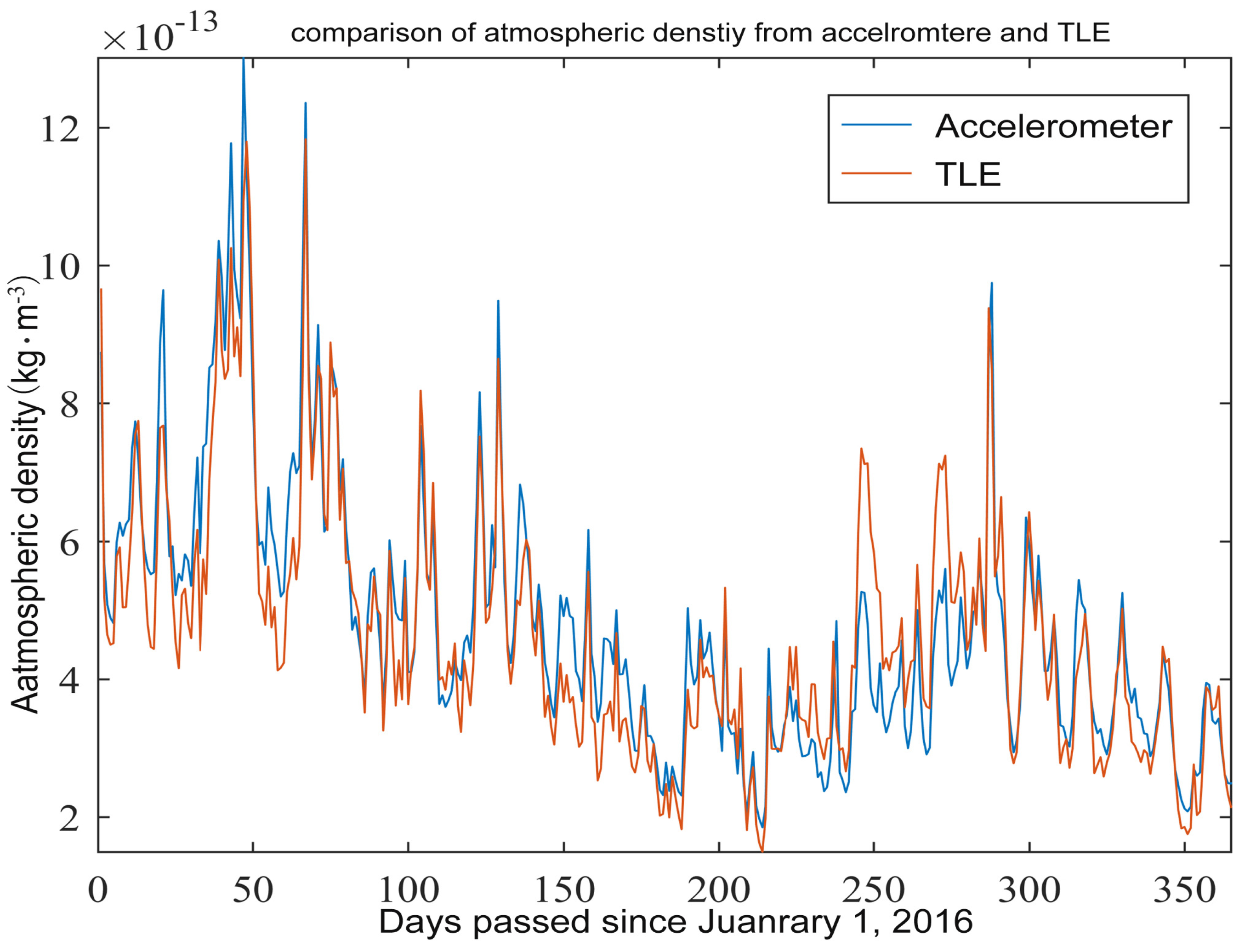
The two-line orbital element data set of Swarm-C and the acceleration data set of Swarm-C for the whole year of 2016 are used for atmospheric density inversion to verify the correctness of the Swarm-C satellite accelerometer atmospheric density inversion results. The comparison results of the thermosphere atmospheric density obtained by the inversion of the two-row orbital element number of the Swarm-C satellite and the thermosphere atmospheric density obtained by the Swarm-C satellite accelerometer are shown in Figure 2.
Due to the small amount of data in the two datasets, the integration time interval is relatively long. Hence, the Swarm-C satellite’s 2016 two-row orbit element summary data set is selected to calculate the data from 1 January 2016 to December 2016. The atmospheric density was calculated on the 30th of the month; the atmospheric density result calculated by the accelerometer is taken as the daily average value and the two-row orbital element number result. Figure 2 shows that the atmospheric density result obtained using the two-row orbital element number is similar to the accelerometer’s atmospheric density result. However, the details are slightly different. The purpose of using the two-line orbital element method for atmospheric density inversion is only to generally verify the correctness of the atmospheric density obtained by the accelerometer. However, this method’s long time interval and scarce data cause its accuracy to be far from the accelerometer’s atmospheric density.
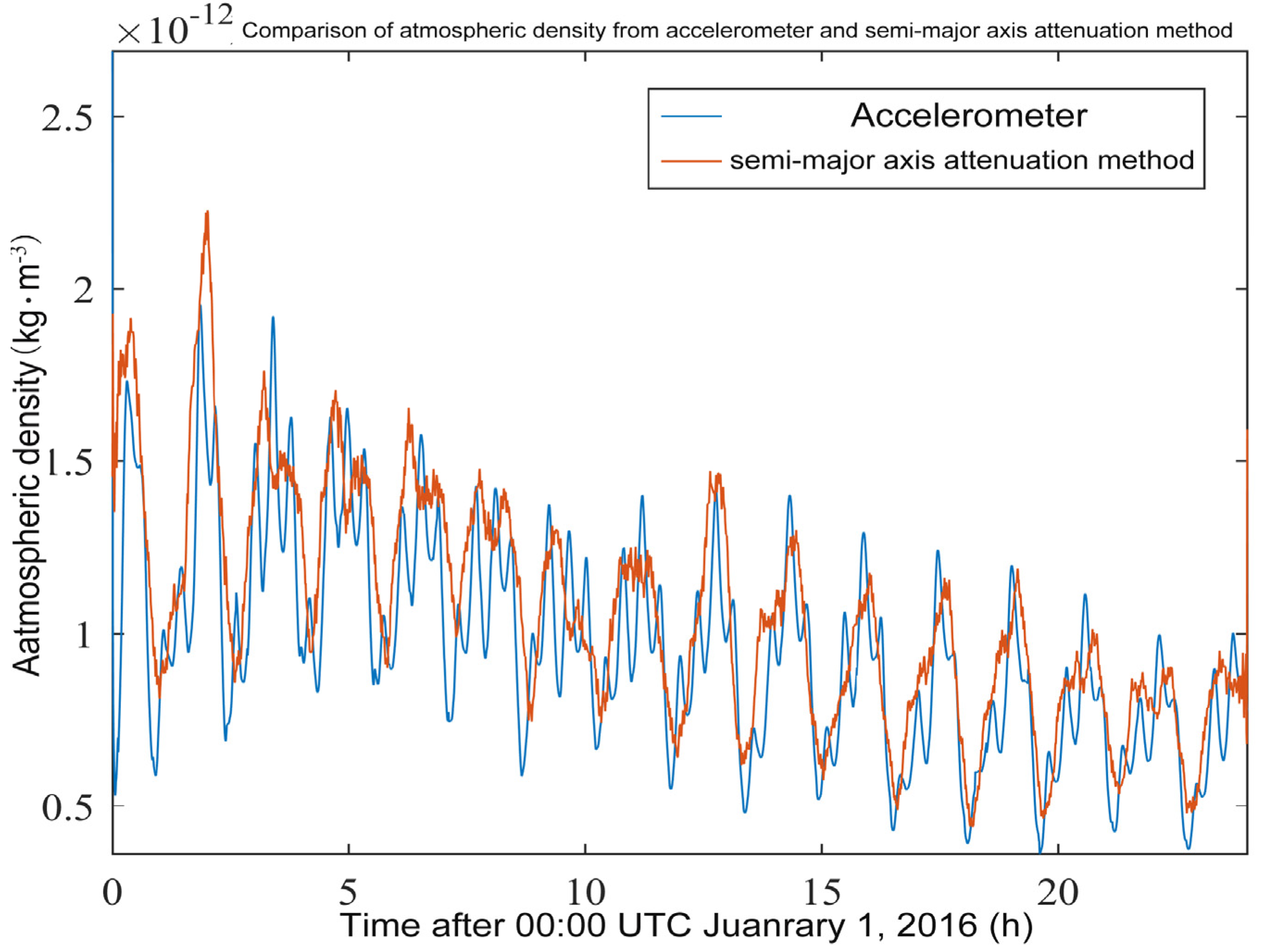
Here, the Swarm-C satellite precision orbit data and the Swarm-C satellite accelerometer data on 1 January 2016 are used for atmospheric density inversion to verify the accuracy and superiority of the atmospheric density retrieved by the Swarm-C accelerometer. Figure 3 compares the long semi-axis attenuation method’s density results and the accelerometer inversion.
The data in Figure 3 comes from the Swarm-C satellite’s LEVEL-2 daily data set on 1 January 2016, including satellite accelerometer data and GPS orbit data. Here, the integration time of the HPOP high-precision orbital integration is 30 s. The figure shows that the atmospheric density obtained by the accelerometer and the atmospheric density obtained by the semi-major axis attenuation method is useful. Furthermore, there is no systematic difference between the two, which verifies the correctness of the atmospheric density results obtained by the accelerometer inversion.

4.2. Swarm-C Accelerometer Inversion Result Evaluation Empirical Atmosphere Model

After the accuracy of atmospheric density is obtained by the Swarm-C satellite, accelerometer inversion is verified. The accelerometer’s atmospheric density can be used to evaluate the existing empirical atmospheric tightness. Furthermore, the consistency between the empirical atmospheric model and the measured atmospheric density can be investigated. Although most of the recognized empirical atmosphere models have been tested and evaluated by different scholars, it is important to further the evaluation and comparison with different data sources. This paper compares the acceleration data with the NRLMSISE-00 and the JB2008 models to further evaluate the selected empirical atmosphere models. After comparing the standard performance, two events of peaking measurement are selected for evaluation on a detailed level.
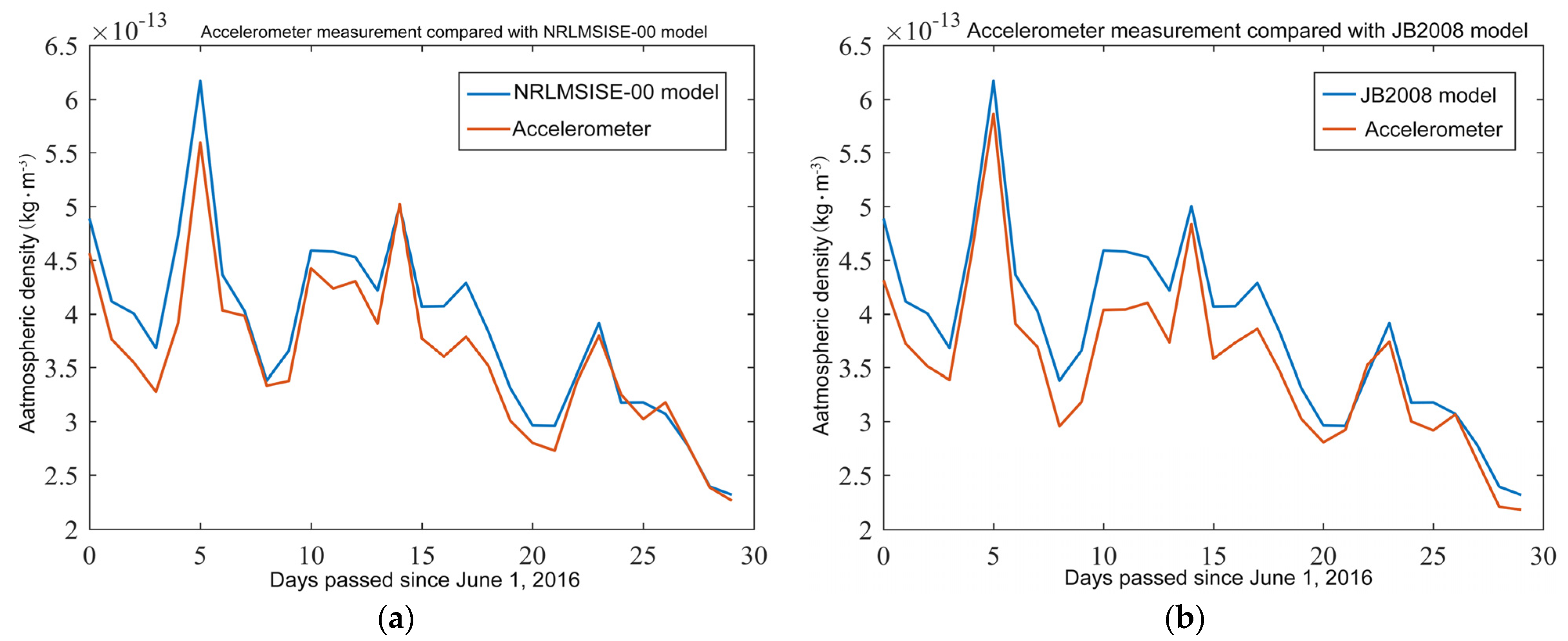
This paper used the acceleration data on 30 June 2016 to calculate the 30-day average daily atmospheric density. Then, the NRLMSISE-00 atmospheric model and the JB2008 atmospheric model are used to obtain the 30-day average daily atmospheric density. Figure 4 shows the comparison between the atmospheric density modeled by the NRLMSISE-00 atmospheric model and the JB2008 atmospheric model and the daily average atmospheric density of the accelerometer.
From Figure 4a, the atmospheric density obtained by the NRLMSISE-00 atmospheric modeling is greater than the atmospheric density measured by the accelerometer for the rest of the period, except for 14 June and 26–28 June. There is a very high peak near 5 June, and the measured atmospheric acceleration density shows a very high peak. However, the two peaks are not equal.
As can be seen from Figure 4b, the trends of the two curves are relatively similar. The accelerometer-measured atmospheric density is smaller than the JB2008 atmospheric model-measured atmospheric density for all time periods except for 22–23 June. In other words, the atmospheric density measured by accelerometers was mostly lower than that obtained by the JB2008 atmospheric model modeling in June 2016. In particular, the difference between the accelerometer-measured atmospheric density and the atmospheric density measured by the JB2008 atmospheric model reached a maximum during the period from 10 June to 14 June. However, during the three peak periods in June, the difference between the accelerometer-measured atmospheric densities and those obtained by the JB2008 atmospheric model is relatively small.
Assuming that the models and parameters in the previous correction process and inversion process are accurate enough, the atmospheric density obtained using the accelerometer can be used as an accurate atmospheric density value. Compared with the precise value of atmospheric density in June 2016, the minimum absolute error of atmospheric density obtained by the NRLMSISE-00 atmospheric model is 0.19%. The maximum is 17.24%. On the other hand, the minimum absolute error of atmospheric density obtained by the JB2008 atmospheric model is 0.18%, and the maximum is 13.04%.
To further investigate the relationship between the atmospheric density obtained by the NRLMSISE-00 model, the JB2008 model, and the actual accelerometric atmospheric density, we used the atmospheric density obtained from the accelerometer as the Y coordinate and the atmospheric density obtained through the simulation of the NRLMSISE-00 atmospheric model and the JB2008 model as the X coordinate to plot the scatter plot. This is shown in Figure 5. The atmospheric density obtained by the accelerometer and the atmospheric density obtained by modeling the NRLMSISE-00 atmospheric density model is highly correlated. The Pearson correlation coefficient of the two is calculated to be 0.9528. The atmospheric density obtained by the accelerometer and the atmospheric density obtained by modeling the JB2008 atmospheric density model is also highly correlated. The Pearson correlation coefficient between the two is calculated to reach 0.9806.
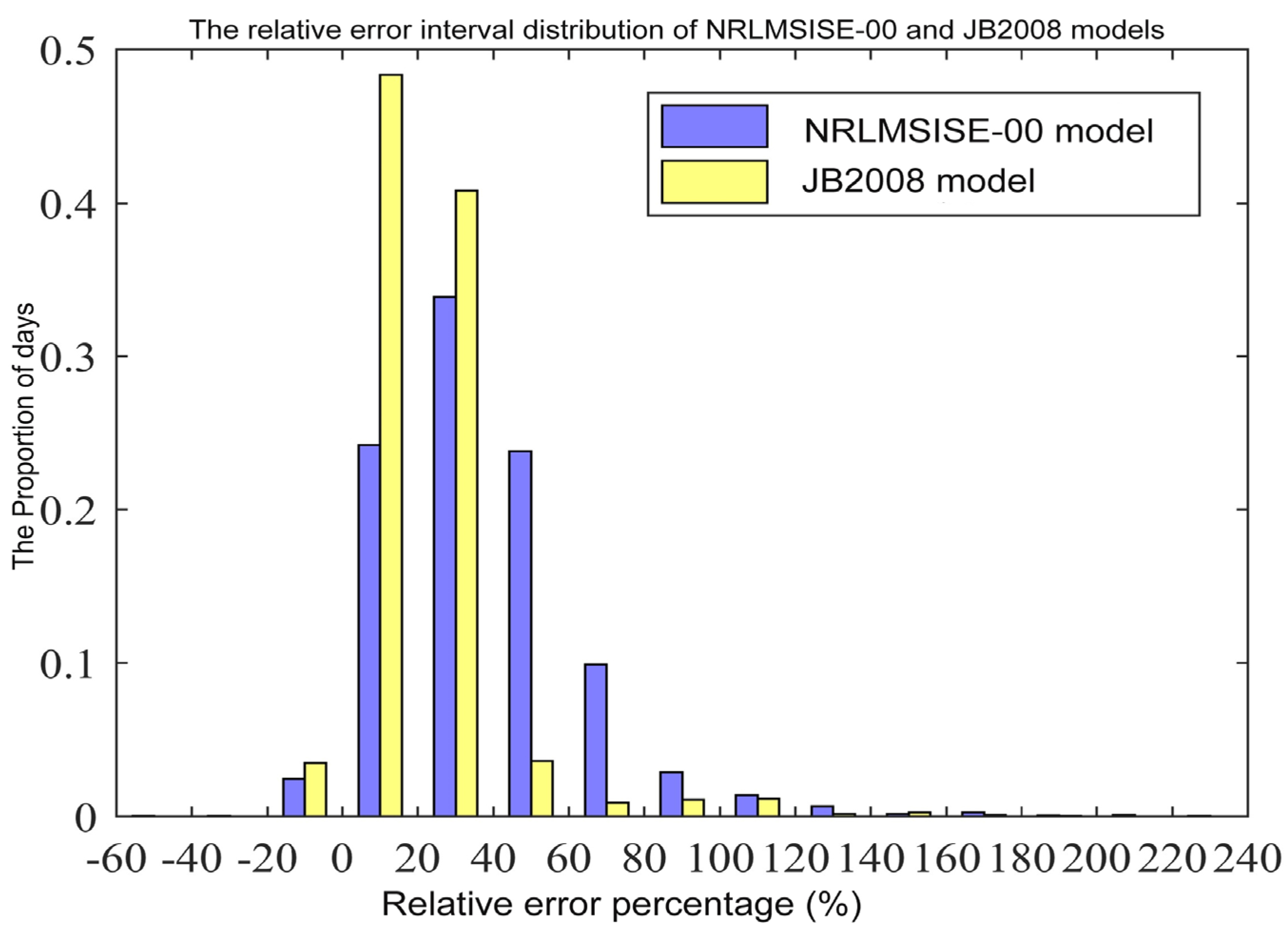
Suppose the thermosphere atmospheric density obtained by the Swarm-C satellite accelerometer in this article is taken as the actual measured value. In that case, the JB2008 empirical model’s modeling results and the NRLMSISE-00 empirical model can be verified and evaluated using the actual measured accuracy values obtained from the accelerometer. Therefore, the relative errors during the two years from 2016 to 2017 between the JB2008 atmospheric model, NRLMSISE-00 atmospheric model, and the Swarm-C satellite accelerometer’s data are counted here. Figure 6 shows the interval distribution of the two model errors.
From Figure 6, for the two-year statistical data of 2016 and 2017, the JB2008 empirical atmosphere model’s relative error distribution is more concentrated than that of the NRLMSISE-00 empirical atmosphere model. It shows that the relative error of the JB2008 atmospheric model is more stable and less floating. It is worth noting that whether it is the JB2008 model or the NRLMSISE-00 model, these two models’ modeling results are likely to be overestimated relative to the actual measurement results. The maximum relative error even exceeded 220%. By comparing with the JB2008 model, the NRLMSISE-00 model has a more severe overestimation of the measured density. From the perspective-relative-error, the lower and upper limits of the relative error distribution interval of the JB2008 atmospheric model are smaller than the NRLMSISE-00 atmospheric model. The correlation coefficient of the JB2008 atmospheric model is also higher than that of the NRLMSISE-00 atmospheric model.
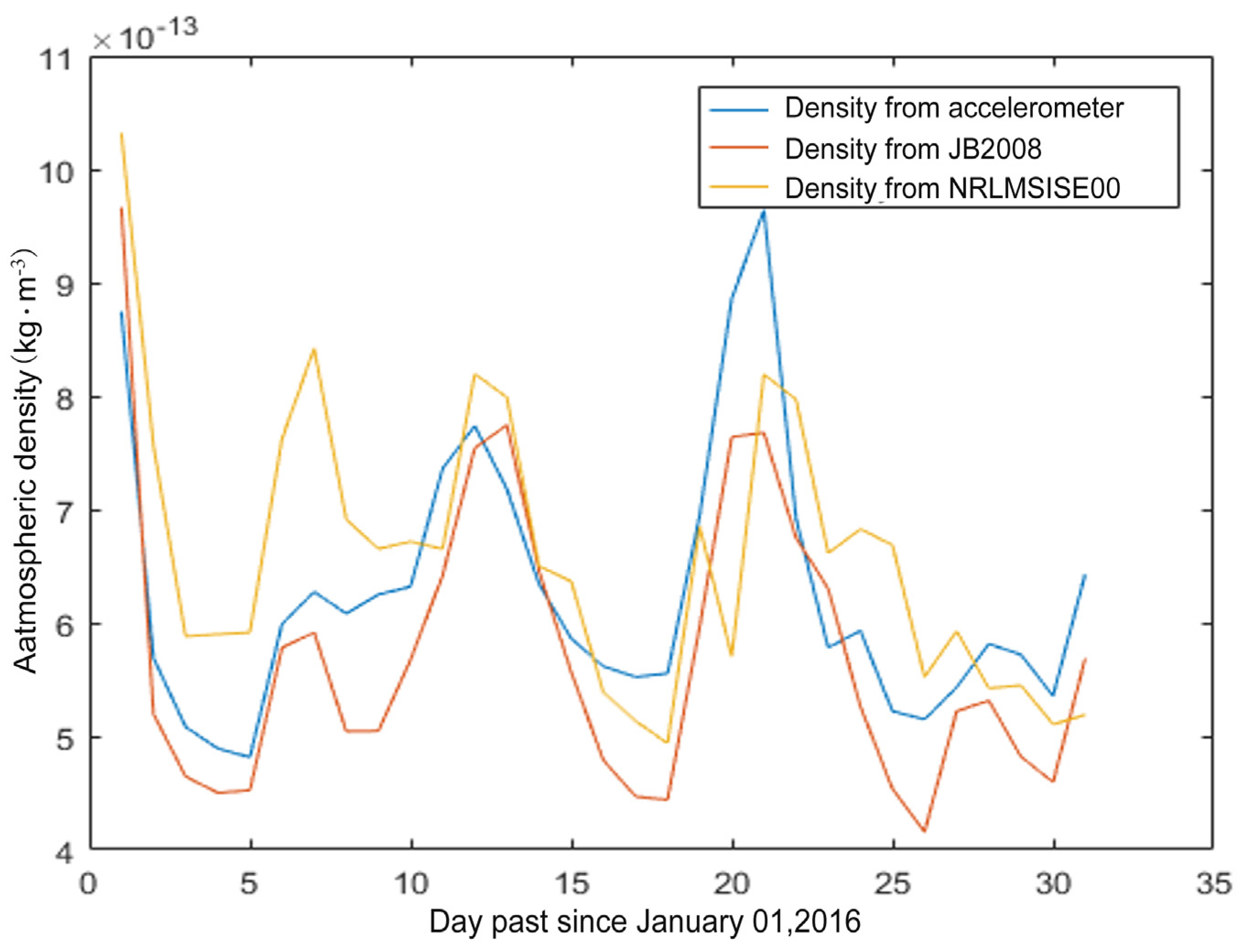
Figure 7 shows the daily average values of the density simulated by the NRLMSISE00 model and the density simulated by the JB2008 model based on the accelerometer data from 1 January 2016 to 31 January 2016. As we can see in the Figure, the three curves are similar. On the 1st, 15th, 22nd, and 27th days, the density curve based on the accelerometer is located in the middle of the other two curves from the classic models. On the 16th and 21st days, the density curve based on the accelerometer was higher than the other two curves and peaked. The accelerometer-based density has the same trend as the classic model in the long run.
The critical concern for the empirical atmospheric model is the model’s accuracy and the atmospheric model’s real-time nature. That the atmospheric model can quickly respond to atmospheric density changes is also crucial for evaluating the model. Two peaks of atmospheric density in June 2016 are selected here, namely the peak near 5 June and the peak near 12 June. This process evaluates the two atmospheric models’ real-time performance to investigate the JB2008 empirical atmosphere model’s real-time performance and the NRLMSISE-00 empirical atmosphere model. Figure 8 shows the time comparison between the JB2008 atmospheric model’s peak values and the NRLMSISE-00 atmospheric model, and the accelerometer’s atmospheric density peak.
It can be seen from Figure 8 that the peak values of the JB2008 atmospheric model and the peak value of the NRLMSISE-00 atmospheric model are delayed relative to the peak value measured by the accelerometer. For the 5 June peak, the JB2008 atmospheric model atmospheric density peak was delayed by 4.3 h from the accelerometer-measured density peak. The NLRMSISE-00 atmospheric model atmospheric density peak was delayed by about 5.2 h from the accelerometer-measured density peak. For the peak near 14 June, the JB2008 atmospheric model atmospheric density peak was delayed by 0.6 h from the accelerometer-measured density peak. The NRLMSISE-00 atmospheric model atmospheric density peak was delayed by 1.5 h from the accelerometer-measured density peak.

5. Discussion

We found some results from the experiment evaluating the NRLMSISE-00 atmospheric model in the Swarm-C inversion result and evaluating the JB2008 atmospheric model in the last section’s Swarm-C inversion result. Therefore, considering the above experimental results, we can propose the following discussion in this section:
(1)
The two-line orbital element method was proposed in the verification experiment of the Swarm-C TLE results and Swarm-C accelerometer results. However, neither this method nor the semi-major axis attenuation method takes the light radiation pressure disturbance term into account. This method is only suitable for space objects below 1000 km because the reverse resistance of the atmosphere mainly causes an object’s resistance with an orbit of less than 1000 km. Once the object’s orbit is higher than 1000 km, the proportion of the light radiation pressure in the satellite’s resistance will increase. The error of the average translation term in the two-row orbit element data set will become more significant, so this method’s atmospheric density will be inaccurate. The radiation pressure model must be introduced if this method is used at altitudes above 1000 km. Because this is not the primary method studied in this article, no more detailed research will be done. The two-line track element data set is designed to facilitate data communication in the early period when communication is underdeveloped. It was used more in the early 1950s and 1980s. Due to the lack of data, the two-line orbital element number is now used for anti-ballistic coefficient and atmospheric density verification. It is a reference for the atmospheric density results obtained by precision orbits or accelerometers. However, its accuracy cannot meet the requirements when performing precise quantitative calculations;
(2)
In the Swarm-C accelerometer’s verification experiment using the results of the Swarm-C semi-major axis attenuation method, the use of the semi-major axis attenuation method requires high-precision HPOP orbit integration to obtain the average value of the semi-major axis changes in a minimal time range. The atmospheric density obtained by the semi-major axis attenuation method is the average atmospheric density during the integration time. Therefore, the semi-major axis attenuation method has low sensitivity and real-time performance compared with the accelerometer’s direct measurement of the atmospheric density. This feature can be seen in Figure 2. The semi-major axis attenuation method’s red density curve fluctuates much less than the accelerometer’s blue density curve. However, the real-time performance of the atmospheric density obtained by the semi-major axis attenuation method is not as good as that obtained by the accelerometer. Compared with the TLE method, the sampling frequency of the semi-major axis attenuation method satellite orbit data is much higher than the sampling frequency of the TLE two-line orbit element data. Although the semi-major axis attenuation method’s dynamics are not as good as the accelerometer’s atmospheric density, it is still better than the atmospheric density obtained by the two-line orbital element;
(3)
In the verification experiment of accelerometer results using the inversion results of Swarm-C orbit data, the results using accelerometer data are directly consistent with the results based on the semi-major axis change. It confirms the correction of the accelerometer calibration and the inversion of density. However, compared to the method that uses accelerometer data directly, the method based on the semi-major axis change is less dynamic. The use of accelerometers to extract atmospheric density has good real-time and dynamic properties. The extraction of atmospheric density using two-line orbital elements and atmospheric density extraction using the semi-major axis attenuation method are essentially the same. Both need to calculate the satellite’s semi-major axis change rate. Since the two-row orbit element data set does not contain satellite position parameters, calculating the atmospheric density by using the two-row orbit element number is necessary to calculate the satellite’s position and speed in the orbit parameters. However, because the two-row track element’s data sampling frequency is far lower than the accelerometer data sampling frequency, CelesTrak publishes only 1–2 sets of two-row orbit element data Swarm-C daily; the data that can be obtained is minimal. Therefore, the integration interval during orbital integration will be considerable. The integration interval selected here is 3 days, so the calculated satellite position and velocity errors are relatively large.
Therefore, it can be found that the use of accelerometers to extract atmospheric density has better real-time and dynamic properties because the accelerometer measures instantaneous non-conservative force acceleration. However, this method requires accurate accelerometer calibration and accurate modeling of the light radiation pressure on the satellite surface. This study used the method to calibrate and correct the accelerometer. Since the deviation caused by other hardware issues is still not considered, errors will inevitably be introduced in the calibration process. It is also the primary source of the accelerometer’s error in extracting atmospheric density. Besides, there are errors caused by illumination radiation pressure modeling. However, this type of error is much smaller than the error introduced in the calibration process. Suppose ESA provides correction methods or corrected data. In that case, the accuracy of the atmospheric density extracted by the accelerometer will also be significantly improved;
(4)
In the experiment of evaluating the NRLMSISE-00 atmospheric model from the Swarm-C inversion results, Figure 5a shows a high degree of correlation between the atmospheric density obtained by using the accelerometer and the atmospheric density obtained by using the NRLMSISE-00 atmospheric density model. After calculation, the Pearson correlation coefficient of the two is 0.9528. According to general experience, if the Pearson coefficient is between 0.0–0.2, the two are irrelevant. Between 0.2–0.4, the two are weakly related. Between 0.4–0.6, the two are moderately correlated. Between 0.6–0.8, the two are strongly correlated. Between 0.8–1.0, the two are highly correlated. It shows that the atmospheric density obtained by the NRLMSISE-00 atmospheric model modeling and the accelerometer’s atmospheric density are already strongly correlated;
(5)
In the Swarm-C inversion results experiments to evaluate the JB2008 atmospheric model, Figure 5b shows the correlation degree of atmospheric density obtained using the accelerometer and JB2008 atmospheric density model higher than that of the accelerometer and NRLMSISE-00. After calculation, the Pearson correlation coefficient of the two has reached 0.9806. The Pearson correlation coefficient is more significant than 0.8, a robust correlation. It shows that the atmospheric density obtained by the JB2008 atmospheric model modeling and the accelerometer’s atmospheric density is strongly positively linear related;
(6)
In the experiment of evaluating the accuracy and real-time performance of the two atmospheric models, the JB2008 atmospheric model has a smaller delay and a faster response than the NRLMSISE-00 model. However, the NRLMSISE-00 model has also estimated some characteristics that the JB2008 model misses. On the whole, among the two peaks, the atmospheric density peak measured by the accelerometer is higher than the atmospheric density peak obtained by the two atmospheric models. Although the difference between the peak of the atmospheric model of NRLMSISE-00 and the accelerometer’s density is larger than that of JB2008, the NRLMSISE-00 has a better performance in estimating the overall pattern. Depending on the different expectations and usage, both models would have drawbacks and benefits. Moreover, the differences in performance accuracy are different in the two selected events. For example, the JB2008 model has a much better performance on 5 June than NRLMSISE-00, while 14 June is very similar. The model accuracy change may cause this phenomenon due to the solar cycle change. Depending on the different backgrounds and circumstances, the two models can be beneficial on different occasions. By understanding how the two model performance differs from different satellite data, the community would have a better understanding of how and what to use for their future studies;
(7)
From the experiment of using Swarm-C accelerometer inversion results to evaluate the empirical atmosphere model, it can be found that at the position where the Swarm-C satellite is flying, using the JB2008 atmospheric model for modeling will achieve better results than using the NRLMSISE-00 model, which means that the accuracy of the JB2008 atmospheric model at the altitude of the Swarn-C satellite is better than that of the NLRMSISE-00 atmospheric model. The altitude of Swarm-C satellite flight is about 500 km from the surface. It also verifies that the JB2008 atmospheric model proposed by Bruinsma et al. has a better simulation effect at altitudes below 500 km than the NRLMSISE-00 atmospheric model. The NRLMSISE-00 atmospheric model performs better than the JB2008 at altitudes above 500 km. This is because solar radiation has a heating effect on the atmosphere. The JB2008 atmospheric model considers the four bands of sunlight’s influence on the atmospheric density and corrects it. It also responds quickly to auroral heating. This is why the JB2008 atmospheric model has a better modeling effect here. It should be noted that the above discussion on the accuracy and real-time performance of the empirical atmosphere model is based on the geomagnetic calm period. However, the accuracy will change for periods of geomagnetic activity or magnetic storms. Therefore, the above results may not be valid [32].

6. Conclusions

This paper uses the two-row orbital elements density inversion to verify the atmospheric density accuracy results of the Swarm-C satellite accelerometer. After the accuracy of the satellite data is verified, this paper conducts comparative verification and empirical atmospheric model evaluation experiments based on the Swarm-C accelerometer’s inversion results.
The correctness of the inversion result of the Swarm-C accelerometer is verified by the inversion result of the two-line orbital elements. After comparing the inversion results of the Swarm-C semi-major axis attenuation method, the accelerometer’s advantages to invert the atmospheric density are analyzed. It is found that the real-time and dynamic nature of the atmospheric density inverted by using the Swarm-C accelerometer is better. Then, using the Swarm-C accelerometer inversion results to evaluate the two empirical atmospheric models, it is found that at the orbital height of the Swarm-C satellite, the JB2008 model has better accuracy and real-time performance than the NRLMSISE-00 model, unlike other satellites in a higher altitude.
This paper has made some progress in using Swarm-C accelerometer inversion results to evaluate empirical atmospheric model experiments. However, there are still some shortcomings, which can be further studied and promoted.
Because it is impossible to understand all the Swarm-C satellite accelerometer’s hardware conditions and failure causes, this article’s accelerometer calibration method cannot correct the errors caused by the accelerometer’s hardware problems. As a result, the accelerometer’s accuracy and the empirical atmosphere models still need improvement. With the improvement of deep learning, a higher-precision correction algorithm needs to be developed and announced by ESA. ESA will regularly publish the corrected accelerometer data of the Swarm satellite. However, the frequency of data updates is not high, and the time delay is considerable. Therefore, it is hoped that ESA can provide a higher-precision correction method or publish the corrected accelerometer data results in a timelier manner, providing convenience for researchers in scientific research.

Author Contributions

Conceptualization, W.Z., L.W. and L.Y.; methodology, L.G. and J.T.; software, L.G. and J.T.; validation, L.G., J.T. and Y.L.; formal analysis, S.L. and B.Y.; investigation, Y.L.; resources, W.Z.; data curation, L.G. and J.T.; writing—original draft preparation, L.Y.; writing—review and editing, L.Y. and W.Z.; visualization, J.T. and L.G.; supervision, B.Y.; project administration, B.Y.; funding acquisition, W.Z., All authors have read and agreed to the published version of the manuscript.

Funding

This work was supported by the Sichuan Science and Technology Program (2021YFQ0003).

Institutional Review Board Statement

Not applicable.

Informed Consent Statement

Not applicable.

Data Availability Statement

The Swarm satellite data used for the study are open source data provided by the European Space Agency https://earth.esa.int/eogateway/missions/swarm accessed on 7 December 2018.

Acknowledgments

The authors express their sincere appreciation and profound gratitude to research assistants Zhiyang Ma and Xiangjun Liu for their help and support in collecting and sorting the data.

Conflicts of Interest

The authors declared no potential conflict of interest with respect to the research, authorship, and/or publication of this article.

References

  1. Emmert, J.T.; McDonald, S.E.; Drob, D.P.; Meier, R.R.; Lean, J.L.; Picone, J.M. Attribution of interminima changes in the global thermosphere and ionosphere. J. Geophys. Res. Space Phys. 2014, 119, 6657–6688. [Google Scholar] [CrossRef]
  2. Vickers, H.; Kosch, M.J.; Sutton, E.; Bjoland, L.; Ogawa, Y.; La Hoz, C. A solar cycle of upper thermosphere density observations from the EISCAT Svalbard Radar. J. Geophys. Res. Space Phys. 2014, 119, 6833–6845. [Google Scholar] [CrossRef] [Green Version]
  3. Zurek, R.W.; Tolson, R.A.; Bougher, S.W.; Lugo, R.A.; Baird, D.T.; Bell, J.M.; Jakosky, B.M. Mars thermosphere as seen in MAVEN accelerometer data. J. Geophys. Res. Space Phys. 2017, 122, 3798–3814. [Google Scholar] [CrossRef]
  4. Drob, D.; Emmert, J.; Crowley, G.; Picone, J.; Shepherd, G.; Skinner, W.; Hays, P.; Niciejewski, R.; Larsen, M.; She, C. An empirical model of the Earth’s horizontal wind fields: HWM07. J. Geophys. Res. Space Phys. 2008, 113, A12. [Google Scholar] [CrossRef]
  5. Grivas, G.; Chaloulakou, A. Artificial neural network models for prediction of PM10 hourly concentrations, in the Greater Area of Athens, Greece. Atmos. Environ. 2006, 40, 1216–1229. [Google Scholar] [CrossRef]
  6. Holben, B.N.; Eck, T.F.; Slutsker, I.; Tanré, D.; Buis, J.P.; Setzer, A.; Vermote, E.; Reagan, J.A.; Kaufman, Y.J.; Nakajima, T.; et al. AERONET—A Federated Instrument Network and Data Archive for Aerosol Characterization. Remote Sens. Environ. 1998, 66, 1–16. [Google Scholar] [CrossRef]
  7. Slini, T.; Kaprara, A.; Karatzas, K.; Moussiopoulos, N. PM10 forecasting for Thessaloniki, Greece. Environ. Model. Softw. 2006, 21, 559–565. [Google Scholar] [CrossRef]
  8. Liu, H.; Hirano, T.; Watanabe, S. Empirical model of the thermospheric mass density based on CHAMP satellite observations. J. Geophys. Res. Space Phys. 2013, 118, 843–848. [Google Scholar] [CrossRef]
  9. Bowman, B.; Tobiska, W.K.; Marcos, F.; Huang, C.; Lin, C.; Burke, W. A New Empirical Thermospheric Density Model JB2008 Using New Solar and Geomagnetic Indices. In Proceedings of the AIAA/AAS Astrodynamics Specialist Conference and Exhibit, Honolulu, HI, USA, 18–21 August 2008; p. 6438. [Google Scholar] [CrossRef] [Green Version]
  10. Doornbos, E. Thermospheric Density and Wind Determination from Satellite Dynamics; Springer Science & Business Media: Berlin/Heidelberg, Germany, 2012. [Google Scholar]
  11. Picone, J.M.; Hedin, A.E.; Drob, D.P.; Aikin, A.C. NRLMSISE-00 empirical model of the atmosphere: Statistical comparisons and scientific issues. J. Geophys. Res. 2002, 107, 1468. [Google Scholar] [CrossRef]
  12. Seo, S.; Kim, J.; Lee, H.; Jeong, U.; Kim, W.; Holben, B.N.; Kim, S.-W.; Song, C.H.; Lim, J.H. Estimation of PM10 concentrations over Seoul using multiple empirical models with AERONET and MODIS data collected during the DRAGON-Asia campaign. Atmos. Chem. Phys. 2015, 15, 319–334. [Google Scholar] [CrossRef] [Green Version]
  13. Zheng, W.; Li, X.; Xie, J.; Yin, L.; Wang, Y. Impact of human activities on haze in Beijing based on grey relational analysis. Rend. Lince 2015, 26, 187–192. [Google Scholar] [CrossRef]
  14. Rajendra, P.P.; Kuga, H.K. An evaluation of Jacchia and MSIS 90 atmospheric models with CBERS data. Acta Astronaut. 2001, 48, 579–588. [Google Scholar] [CrossRef]
  15. Xu, J.; Wang, W.; Zhang, S.; Liu, X.; Yuan, W. Multiday thermospheric density oscillations associated with variations in solar radiation and geomagnetic activity. J. Geophys. Res. Space Phys. 2015, 120, 3829–3846. [Google Scholar] [CrossRef]
  16. Murray, S.A.; Henley, E.M.; Jackson, D.R.; Bruinsma, S.L. Assessing the performance of thermospheric modeling with data assimilation throughout solar cycles 23 and 24. Space Weather 2015, 13, 220–232. [Google Scholar] [CrossRef] [Green Version]
  17. Shim, J.; Kuznetsova, M.; Rastätter, L.; Bilitza, D.; Butala, M.; Codrescu, M.; Emery, B.; Foster, B.; Fuller-Rowell, T.; Huba, J. CEDAR Electrodynamics Thermosphere Ionosphere (ETI) Challenge for systematic assessment of ionosphere/thermosphere models: Electron density, neutral density, NmF2, and hmF2 using space based observations. Space Weather 2012, 10, 10. [Google Scholar] [CrossRef] [Green Version]
  18. Bezdek, A. Calibration of accelerometers aboard GRACE satellites by comparison with POD-based nongravitational accelerations. J. Geodyn. 2010, 50, 410–423. [Google Scholar] [CrossRef] [Green Version]
  19. Liu, S.; Gao, Y.; Zheng, W.; Li, X. Performance of two neural network models in bathymetry. Remote Sens. Lett. 2015, 6, 321–330. [Google Scholar] [CrossRef]
  20. Reid, C.E.; Jerrett, M.; Petersen, M.L.; Pfister, G.G.; Morefield, P.E.; Tager, I.B.; Raffuse, S.M.; Balmes, J.R. Spatiotemporal Prediction of Fine Particulate Matter During the 2008 Northern California Wildfires Using Machine Learning. Environ. Sci. Technol. 2015, 49, 3887–3896. [Google Scholar] [CrossRef]
  21. Picone, J.M.; Emmert, J.T.; Lean, J. Thermospheric densities derived from spacecraft orbits: Accurate processing of two-line element sets. J. Geophys. Res. Earth Surf. 2005, 110. [Google Scholar] [CrossRef]
  22. Siemes, C.; Da Encarnação, J.D.T.; Doornbos, E.; Van Den Ijssel, J.; Kraus, J.; Pereštý, R.; Grunwaldt, L.; Apelbaum, G.; Flury, J.; Olsen, P.E.H. Swarm accelerometer data processing from raw accelerations to thermospheric neutral densities. Earth Planets Space 2016, 68, 1–16. [Google Scholar] [CrossRef] [Green Version]
  23. Ijssel, J.V.D.; Doornbos, E.; Iorfida, E.; March, G.; Siemes, C.; Montenbruck, O. Thermosphere densities derived from Swarm GPS observations. Adv. Space Res. 2020, 65, 1758–1771. [Google Scholar] [CrossRef]
  24. Bezděk, A.; Sebera, J.; Klokočník, J. Calibration of Swarm accelerometer data by GPS positioning and linear temperature correction. Adv. Space Res. 2018, 62, 317–325. [Google Scholar] [CrossRef]
  25. Mehta, P.M.; Walker, A.C.; Sutton, E.K.; Godinez, H.C. New density estimates derived using accelerometers on board the CHAMP and GRACE satellites. Space Weather 2017, 15, 558–576. [Google Scholar] [CrossRef]
  26. Weimer, D.; Mlynczak, M.; Emmert, J.; Doornbos, E.; Sutton, E.; Hunt, L. Correlations between the thermosphere’s semiannual density variations and infrared emissions measured with the SABER instrument. J. Geophys. Res. Space Phys. 2018, 123, 8850–8864. [Google Scholar] [CrossRef] [Green Version]
  27. March, G.; Doornbos, E.; Visser, P. High-fidelity geometry models for improving the consistency of CHAMP, GRACE, GOCE and Swarm thermospheric density data sets. Adv. Space Res. 2018, 63, 213–238. [Google Scholar] [CrossRef]
  28. Sentman, L.H. Free Molecule Flow Theory and Its Application to the Determination of Aerodynamic Forces; Lockheed Missiles and Space Co. Inc.: Sunnyvale, CA, USA, 1961. [Google Scholar]
  29. Kodikara, T.; Carter, B.; Zhang, K. The First Comparison Between Swarm-C Accelerometer-Derived Thermospheric Densities and Physical and Empirical Model Estimates. J. Geophys. Res. Space Phys. 2018, 123, 5068–5086. [Google Scholar] [CrossRef]
  30. Qian, L.; Solomon, S. Thermospheric Density: An Overview of Temporal and Spatial Variations. Space Sci. Rev. 2011, 168, 147–173. [Google Scholar] [CrossRef]
  31. Zhou, Y.; Zheng, W.; Shen, Z. A New Algorithm for Distributed Control Problem with Shortest-Distance Constraints. Math. Probl. Eng. 2016, 2016, 1–6. [Google Scholar] [CrossRef]
  32. Calabia, A.; Jin, S. Thermospheric density estimation and responses to the March 2013 geomagnetic storm from GRACE GPS-determined precise orbits. J. Atmos. Solar-Terr. Phys. 2017, 154, 167–179. [Google Scholar] [CrossRef]
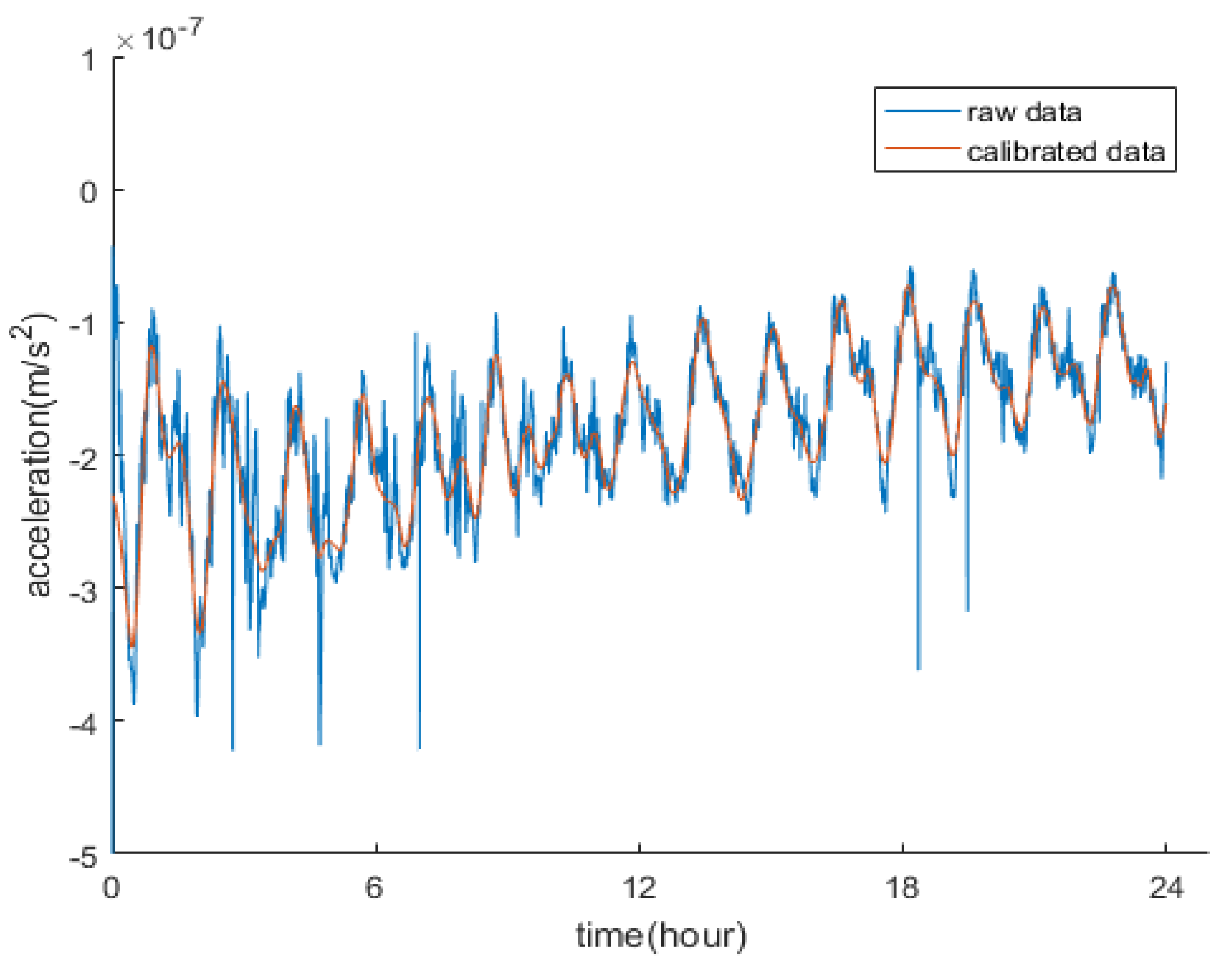
Figure 1. Comparison of data after calibration and raw acceleration by Swarm-C.
Atmosphere 13 00294 g001
Figure 2. Comparison of atmospheric density obtained by the accelerometer and TLE.
Atmosphere 13 00294 g002
Figure 3. Comparison of atmospheric density from the accelerometer and semi-major axis attenuation method.
Atmosphere 13 00294 g003
Figure 4. Atmospheric densities measured by accelerometer compared with results of atmospheric models (a) the NRLMSISE-00 result and the measured atmospheric densities; (b) the JB2008 result and the measured atmospheric density.
Atmosphere 13 00294 g004
Figure 5. Scatter diagram of the relationship between the measured atmospheric density by the accelerometer and atmospheric models (a) Scatter diagram of the measured atmospheric density and NRLMSISE-00; (b) Scatter plot of the measured atmospheric density and JB2008.
Atmosphere 13 00294 g005
Figure 6. The relative error interval distribution of NRLMSISE-00 and JB2008 models.
Atmosphere 13 00294 g006
Figure 7. The daily mean density of accelerometer measurement and two atmospherics models.
Atmosphere 13 00294 g007
Figure 8. Comparison of the two atmospheric models and the measured accelerometer. (a) 5 June 2016 JB2008 model result and accelerometer measurement; (b) 14 June 2016 JB2008 model result and accelerometer measurement; (c) 5 June 2016 NRLMSISE-00 model result and accelerometer measurement; (d) 14 June 2016 NRLMSISE-00 model result and accelerometer measurement.
Atmosphere 13 00294 g008
Publisher’s Note: MDPI stays neutral with regard to jurisdictional claims in published maps and institutional affiliations.