Article

Effect of the Near-Future Climate Change under RCP8.5 on the Heat Stress and Associated Work Performance in Thailand

by
Teerachai Amnuaylojaroen
1,2,*,
Atsamon Limsakul
3,
Sukrit Kirtsaeng
4,
Nichapa Parasin
5 and
Vanisa Surapipith
6,*
1
Department of Environmental Science, School of Energy and Environment, University of Phayao, Phayao 56000, Thailand
2
Atmospheric Pollution and Climate Research Unit, School of Energy and Environment, University of Phayao, Phayao 56000, Thailand
3
Environmental Research and Training Center, Department of Environmental Quality Promotion Technopolis, Klong 5, Klong Luang, Pathumthani 12120, Thailand
4
Thai Meteorological Department, Bangkok 10260, Thailand
5
School of Allied Health Science, University of Phayao, Phayao 56000, Thailand
6
National Astronomical Research Institute of Thailand, Chiang Mai 50180, Thailand
*
Authors to whom correspondence should be addressed.
Atmosphere 2022, 13(2), 325; https://doi.org/10.3390/atmos13020325
Submission received: 28 December 2021 / Revised: 9 February 2022 / Accepted: 10 February 2022 / Published: 15 February 2022
(This article belongs to the Special Issue Extreme Weather, Air Pollution, and Human Health)

Abstract

:
Increased heat stress affects well-being, comfort, and economic activities across the world. It also causes a significant decrease in work performance, as well as heat-related mortality. This study aims to investigate the impacts of the projected climate change scenario under RCP8.5 on heat stress and associated work performance in Thailand during the years 2020–2029. The model evaluation shows exceptional performance in the present-day simulation (1990–1999) of temperature and relative humidity, with R2 values ranging from 0.79 to 0.87; however, the modeled temperature and relative humidity are all underestimated when compared to observation data by −0.9 °C and −27%, respectively. The model results show that the temperature change will tend to increase by 0.62 °C per decade in the future. This could lead to an increase in the heat index by 2.57 °C if the temperature increases by up to 1.5 °C in Thailand. The effect of climate change is predicted to increase heat stress by 0.1 °C to 4 °C and to reduce work performance in the range of 4% to >10% across Thailand during the years 2020 and 2029.

1. Introduction

Global climate change, manifested as a rise in the average global temperature, has emerged as a megatrend that will result in significant ecological and social-economic impacts in the future. According to the Intergovernmental Panel on Climate Change’s (IPCC) Assessment Report on Climate Change, released in 2021, climate change poses a substantial threat to societies around the world, and the changes observed in the climate are widespread, rapid, and intensifying, with some of the changes, such as the continued sea level rise, being irreversible over hundreds to thousands of years. By the end of the century, the global surface temperature is very likely to be 1.0 °C to 1.8 °C warmer under the very low greenhouse gas (GHG) emissions scenario and 3.3 °C to 5.7 °C warmer under the very high GHG emissions scenario [1]. Additionally, by 2100, it is estimated that between half and two thirds of the global population will reside in high-temperature areas, where temperatures will reach a level that is unlivable for humans on several days each year [2]. Intensive weather threatens people’s well-being and cognitive capacity, and the risk of heat-related illness is expected to increase as a result of increased global warming and associated extreme weather events [3,4,5]. Moreover, heat diminishes leisure opportunities and impairs the efficiency of healthy individuals in society, since there are obvious and practical limits to the amount of heat exposure that a person can endure [4,6,7,8,9].
One of the major risks associated with rising temperatures is the possibility of heat-related illnesses and socioecological disasters, which often result in potentially reparable yet devastating economic damage and irreversible human loss [10,11,12,13]. Besides climatic variables, sociodemographic factors have an impact on a population’s vulnerability to heat stress, and their interaction can result in an increase in the degree of exposure to heat-related threats. As reported by Rao et al. [14], future summertime heat stress projected from 18 Coupled Model Intercomparison Project Phase 5 (CMIP5) models, which is a standard experimental framework for studying the output of coupled atmosphere–ocean general circulation models, revealed exceptional increases under the Representative Concentration Pathways (RCPs) 4.5 and 8.5 emission scenarios over India. The predicted heat stress has been determined to have a greater influence on the coastal parts of India, which are more likely to experience days categorized as extreme caution to danger, and a higher risk of occurrence. Rising levels of heat stress across India appear to be related to the severe temperature changes, increases in the duration and intensity of warm days, and future modulation in large-scale circulation. Work performance in India is expected to fall by 30 to 40% by the end of the 21st century due to increases in heat stress levels, posing significant problems for the country’s policymakers in designing safety measures and protecting people continuously working in extremely hot weather conditions.
Southeast Asia (SEA) is one of the regions that is especially vulnerable to extreme heat, interlinking physical and human pressures such as high population density, welfare dependency, low adaptive capability, and a hot and humid climate background [15]. The threat is heightened for approximately 60% of the SEA’s working population, engaged in outdoor activities related to agriculture, the region’s primary economic activity [15,16]. As reported by Krellenberg et al. [17], climate change is inextricably linked to urbanization and is one of the most critical challenges associated with chronic environmental change. In recent years, the SEA has been devastated by a series of deadly heatwaves [18]. For example, in April 2016, there was a prolonged heatwave, with temperatures reaching record highs and causing new national heat records to be set and many others to come dangerously close. Thailand and neighboring countries are experiencing the worst heatwave in the region’s history since 1950. According to the Meteorological Department of Thailand, at least 50 cities in the country experienced all-time high temperatures on 19 April 2016 (available online: https://weather.com/news/weather/news/thailand-southeast-asia-extreme-record-heat (accessed on 27 January 2018)). In addition, Paengkaew et al. [19], who studied the variability and trend of the heat index in Thailand during 1975–2017, indicated that the long-term trend of the heat index in Thailand as a whole significantly increased by 0.53 °C per decade. Despite natural heat acclimatization, deaths from heat stress are a result of the combination of natural and human processes, which adversely increase the risk of heat extremes in this region [20,21,22,23,24].
The current global warming trend is expected to accelerate and expose workers performing tasks in outdoor and indoor workplaces that lack thermal neutrality to physiological acclimatization. There were some previous studies about climate change and heat in SEA—for example, Dong et al. [18], who studied the heatwaves in SEA and their changes in a warmer world, and Paengkaew et al. [19], who studied the heat index in Thailand during 1975–2017. However, there are no studies about climate change and work performance that are related to heat stress, particularly paying attention to urban areas. Because many megacities have high population densities and people are exposed to both high temperatures and humidity during heatwaves, there is a high risk of both heat stress and heat stroke [4]. As Thailand is a country in SEA that is more vulnerable to heat extremes due to expected temperature increases, understanding the effects of future climate change on heat stress and work performance enables policymakers to take steps to protect workers from the harmful exposure to heat stress and sustain work performance [19,25]. This article employs a heat index to predict heat stress and its association with work performance in Thailand. In this study, we selected five highly populated megacities in Thailand, including Chiang Mai, Khon Kaen, Phitsanulok, Bangkok, and Songkhla, to project heat stress and associated work performance. The findings of this study may assist policymakers in developing more effective policy tools for addressing the welfare of working people, who will face increased heat stress as a result of changing climate conditions in the future.

2. Materials and Methods

To deal with the impact of the worst-case scenario of climate change (high emission scenario) on human health in the context of heat risk in Thailand, the climate change scenario RCP8.5 was selected in this study. Moreover, this study selected five Thai megacities: Chiang Mai, Phitsanulok, Khon Kaen, Bangkok, and Songkhla. The 2 m temperature and relative humidity data from the Nested Regional Climate Model (NRCM) simulation under climate change scenario RCP8.5 were utilized as input data to calculate the heat index (HI), and the HI was used as input data to determine the decrement in work performance.

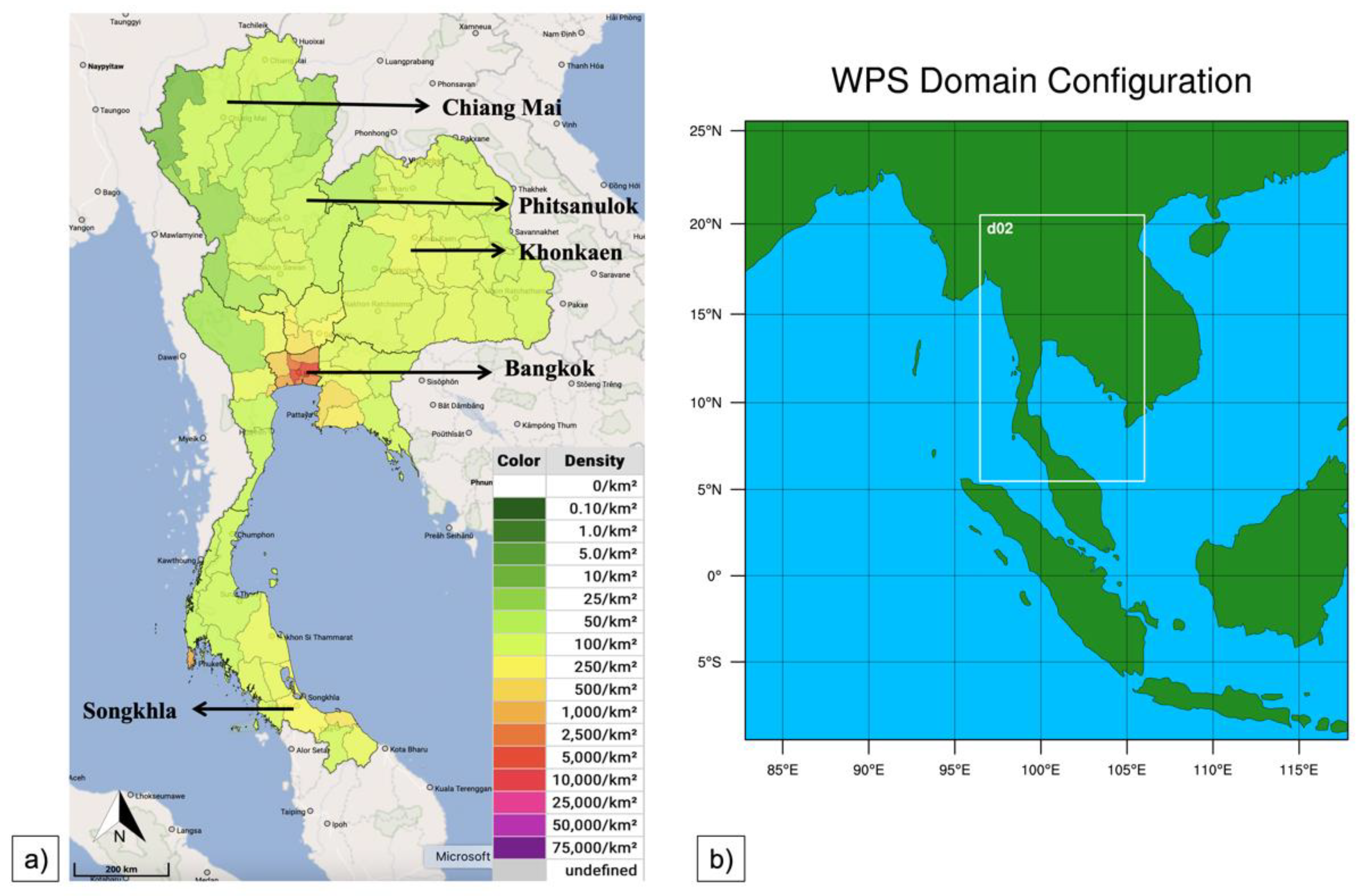
2.1. General Information of Cities in This Study

To quantify the possible effects of climate change on heat stress in the selected cities, we averaged five grid points over each of them, as shown in Figure 1a. According to the data of the year 2019, as listed in Table 1, several Thai megacities, including Chiang Mai, Phitsanulok, Khon Kaen, and Songkhla, have a total population of up to 1.7 million people, while Bangkok, Thailand’s capital, has a population of up to 8.8 million people. Furthermore, Bangkok has a high population density, with 5621 people per km2, while other large cities have population densities ranging from 82 to 211 people per km2. The population density was calculated based on the equation below:
Population density = Number of people Land area in square kilometer

2.2. Information of Output from Nested Regional Climate Model

The HI calculation was performed using the output from the inner domain, including 2 m temperature and relative humidity, from the previous simulation by the NRCM under climate change scenario RCP8.5 [25]. RCP8.5 combines assumptions about high population and relatively slow income growth with modest rates of technological change and energy intensity improvements, leading in the long term to a high energy demand and GHG emissions in the absence of climate change policies. The domain of the previous simulation is shown in Figure 1b. It was configured to have two domains, covering SEA for the outer domain with 60 km grid spacing and Thailand for the inner domain with 10 km grid spacing, while the vertical resolution was set to 53 levels. The previous simulation was run in two cases: (1) in the past period (1990–1999) and (2) in the future period (2020 and 2029). The general model configuration was as follows: the meteorological initial and boundary conditions were implemented with the Community Climate System Model version 4 (CCSM4) [26,27,28]. The NRCM was forced with CCSM4 data that corrected the mean error in the GCM using the bias-corrected method, as described in Bruyere et al. [29]. The interaction between land and ocean was calculated in the model configuration using the Price–Weller–Pinkle (PWP) model, which also determines oceanic parameters [30]. This is a model of the oceanic mixing layer that incorporates convection shift and oceanic shear stability. It was constructed using the vertical mixing model HYCOM [31]. To simulate the feedback and evolution of aerosols in the atmosphere, the Rapid Radiative Transmission Model was used (RRTMG). The Thompson scheme is used in the model to extract information about meteorological processes from aerosols [32]. Grell-3 and the Noah Land Surface Model were used to determine the model’s subgrid scale and the relationship between land and atmosphere [33]. Grid nudging is often used primarily to provide large-scale meteorology [34].
For analysis in the megacities of Thailand, even though 10 km is not enough to represent micro-scale processes on an urban scale, it could basically capture the mesoscale processes that represent most countries in the context of climate. In addition, to resolve the sub-grid scale process, i.e., an urban process in the model, the urban canopy model calculation in the land surface model, which is based on the Noah Land Surface Model, was enabled in the simulation. Regarding the land area of Thailand, which amounts to approximately 514,000 km2, the 10 km grid spacing in the model output was not a problem to represent the atmospheric process. However, it is not a good representation of urban meteorology, since it should be less than 1 km. Moreover, 10 km of grid spacing mostly covers all municipal areas in this study.

2.3. Quality Control and Homogeneity Checks

The quality and homogeneity of observation data in Thailand from 1990 to 1999 were statistically tested using commonly used methods [35]. Before being eliminated, outliers in each data series were identified by comparing their values to adjacent days and to the same day at nearby stations. The second step was to evaluate data homogeneity using the penalized t-test and the penalized maximal F-test. These methods can detect multiple step changes in time series by comparing the goodness of fit of a two-phase regression model to that of a linear trend over the entire base series [36,37]. The homogeneity tests indicated 82 inhomogeneous temperature and relative humidity data. A relative inhomogeneity correction was used, in which the candidate series was compared to the adjacent homogeneity stations [38]. The reference series was chosen from the homogeneous adjacent stations that were well correlated with the inhomogeneous data. The data set of 44 high-quality records was used for model evaluation after the quality control procedure and homogeneity tests.

2.4. Heat Index and Decrements in Work Performance

Many studies on heat stress use only temperature data and not humidity data [39,40,41]. However, humidity plays an essential role in the discomfort caused by warmth and must be considered when calculating the heat stress index [2,42,43], especially in tropical regions. Several methods are used to quantify heat stress depending on different environmental and meteorological variables. Some indicators combine temperature and moisture, such as the National Weather Service Heat Index and Humidex [44], while others include solar radiation (e.g., wet bulb globe temperature (WBGT) [45] and the Environmental Stress Index [46]). Steadman’s apparent temperature is one of the most commonly used thermal indices in environmental health studies [47]. It is entirely based on temperature and moisture and is sometimes referred to as the “heat index”. One of its benefits is that it is a straightforward index that may be used to investigate variability and long-term change. For example, Paengkaew et al. [19] employed the HI to investigate the long-term trend in Thailand from 1975 to 2017. Moreover, Wang et al. [48] used temperature and humidity to develop a heatwave warning system in rural and urban areas in Alabama, USA [49]. Meanwhile, Bohmanova et al. [50] used both temperature and humidity to determine the threshold of heat stress and rate of decline of milk production in Phoenix, Arizona and Athens, Georgia.
We employed Steadman’s HI [47] to calculate the heat stress in this study. The HI was calculated by combining the relative humidity and temperature as developed by Rothfusz [47] as follows:
HI = −42.379 + 2.04901523(T) + 10.14333127(RH) − 0.22475541(T)(RH) − 0.00683783(T2) − 0.05481717(RH2) + 0.00122874(T2)(RH) + 0.00085282(T)(RH2) − 0.00000199(T2)(RH2)
where T is air temperature (°C), and RH is relative humidity (%). The HI values were then converted to the Celsius scale and applied to this study. The health effect-based categories of HI values are listed in Table 2.
It is known that extreme heat events lead to a drastic decline in work productivity, along with heat-related mortality [51]. According to Rao et al. [14], a relationship between working performance and thermal comfort has been constructed based on experimental data sets, and a decrement in work performance (P in %) has been found with an increase in temperature. Temperature and HI values are reported to vary little in many regions, and the sensitivity of heat–health effect estimations does not show greater variations when comparing HI with temperature exposure, as shown by Vaneckova et al. [52], who evaluated the performance of several common biometeorological indices including apparent temperature, relative strain index, Thom discomfort index, the humidex and wet-bulb globe temperature, and temperature while investigating heat-related mortality in Brisbane, Australia. They reported that the average temperature performed similarly to the composite indices, but minimum and maximum temperatures performed relatively poorly. Thus, the average temperature may be suitable for the development of weather–health warning systems. Moreover, Anderson and Bell [53] reported that the intensity or duration of heatwaves raises the likelihood of death. Although there is some variance, especially during the summer, a significant correlation between temperature and HI indicates the same quantitative outcomes. To perform our heat–health research, we employed the HI rather than the temperature because heat stress is a stronger indicator. Consequently, the following equation was used to estimate the decrement in work performance as follows:
P (%) = 2 × (HI, °C) − 50
where P is a decrement in work performance (%), HI is a heat index (°C)

2.5. Statistical Used

In addition, the model was evaluated for reliability using statistical analysis, including R-squared, mean bias error, standard deviation of residuals, correlation coefficient, and root mean square error. The mean bias was calculated as follows Equation (2):
Mean Bias   =   1 n 1 n ( M O )
where M is the model data, and O is the observed data. The standard deviation of residuals (SDR) was calculated as follows Equation (3):
SDR = [ ( x O X M ) ( X O ¯ X M ¯ ) ] 2 n
where X O is the observed data, X M is the model data, X O ¯ is the mean of the observed data, X M O ¯ is the mean of the model data, and n is the number of values in the model and the observed data.
The Pearson correlation coefficient was calculated following Equation (4):
r = ( x i x ¯ ) ( y i y ¯ ) ( x i x ¯ ) 2 ( y i y ¯ ) 2
where r is the correlation coefficient.
The root mean square error was calculated using Equation (5):
Root Mean Square Error ( RMSE ) = 1 n ( M O ) 2 n
where M is the model data, and O is the observed data.

3. Results and Discussion

3.1. Model Evaluation during 1990–1999

Figure 2 and Figure 3 show the validation of the difference in monthly mean temperature averaged over 1990–1999 between the model and the observations, based on 44 TMD stations’ locations. In general, the NRCM reasonably predicts the monthly temperature, relative humidity, and HI. The modeled temperature exhibits a cold bias in January–February and November–December, whereas relative humidity and HI are predicted to be lower throughout the year. When validated with ground-based TMD observations data, the spatial distribution of monthly mean relative humidity and 2 m temperature from the inner domain of the NRCM outputs is comparable and well predicted. Although the temperature of the NRCM was higher than that of the TMD by 2 °C–3 °C in most regions of Thailand, especially in March to May, a slight difference in the modeled temperature of −1 °C–−2 °C was found in Northern Thailand for the entire year. An overestimation of the modeled temperature was found in the central part of Thailand for an entire year in the range of 3 °C–5 °C. The HI prediction can be influenced by a temperature bias. Although the HI is affected by two factors—temperature and relative humidity—several studies show that temperature has a strong correlation with the heat index [19,54,55]. There was a lower HI estimation in Northern Thailand, while the higher temperature predicted in Central Thailand led to a higher HI value.
In general, the modeled relative humidity agreed fairly well with that of the observed TMD dataset. The difference in relative humidity between the modeled and the observed TMD data was in the range of (−5)%–(−1)% in the dry season and in the range of (<−5)%–(>5)% in the rainy season. The model agreed with the observations not only in terms of regional distribution, but also in terms of climate pattern. Figure 2 and Figure 3 depict the difference between the monthly modeled 2 m temperature and relative humidity and the observations. The modeled 2 m temperature was lower than the observations for most of the year, with the exception of March, April, and May, indicating a hot bias of the 2 m temperature. The modeled relative humidity was also lower than the observed values for the entire year. Table 3 shows the statistical calculation in the annual mean of temperature, relative humidity, and HI averaged over 1990–1999 between the model and the observations, based on 44 TMD stations’ locations. As demonstrated by the R-squared values ranging from 0.79 to 0.87, the model had a good ability to capture all variables, including temperature, relative humidity, and HI. Meanwhile, the correlation coefficient (CC) was in the range of 0.89–0.92. The modeled temperature, relative humidity, and HI were all underestimated when compared to the observed data, with a mean bias error of (−0.9) °C, (−27)%, and (−23), respectively. For temperature, relative humidity, and HI, the standard deviation of the model’s residuals was 4.1 °C, 29%, and 25, respectively. Meanwhile, the RMSE was 1.70, 4.73, and 23.43 for temperature, relative humidity, and HI, respectively.
To summarize, the NRCM has a strong capacity to predict climatic patterns in this region, as demonstrated above. It reasonably depicts the simulated temperature and relative humidity. However, when compared to the observations, the model consistently underestimates the relative humidity. The simulation of the model’s underestimation of temperature and relative humidity is similar to that of other research, such as Zhang et al. [56], who investigated the impact of weather and season variation on WRF dynamical downscaling in the Pearl River Delta Region, China. Based on their findings, WRF dynamical downscaling had a comparatively lower performance under wet conditions or in tropical regions due to dynamic or physical process deficiencies in the model itself [57]. In general, surface exchange in the land surface model plays a key role in controlling the land surface temperature and humidity. However, uncertainties exist in land data, and land surface variables are depicted coarsely in mesoscale atmospheric numerical models [58,59]. Furthermore, because the model relies on grid nudging to maintain the large-scale meteorology from the Global Climate Model, the errors from the beginning and boundary conditions are crucial to examine. Because the NRCM simulation uses the CCSM4 as the initial and boundary condition, as mentioned in Geng et al. [28] and Yang et al. [60], sea surface temperatures are found in the CCSM4 across the Indian Ocean, which has a substantial influence on the Asian monsoon and likely led to the cold bias in the model simulation. Meanwhile, temperature and relative humidity overestimation lead to a lower estimated HI value when compared to the observations.

3.2. The Relationship between Heat Index, Relative Humidity, and Temperature during 2020–2029

The relationship between HI, relative humidity, and temperature was revealed using a time series of daily averages of these variables over Thailand during 2020–2029. As shown in Figure 4a, the temperature and relative humidity exhibited opposing patterns; when there were high temperatures, the relative humidity tended to decrease, whereas at low temperatures, the relative humidity acquired greater values. This confirmed the role of water vapor in ambient air temperature as a moisture content source [61,62,63]. The temperature and HI, on the other hand, showed a positive correlation trend. When the temperature rose, the HI increased as well. This result indicates that temperature is the main factor that influences the HI over Thailand during 2020–2029.
The average annual temperature in Thailand has increased by 0.62 °C per decade (Figure 4b). The temperature change tends to increase almost throughout the year, except during January, February, and November. A peak increase was found at the end of the year of 2.5 °C, while a reduction in temperature of −1.5 °C was found in February. The average annual HI in Thailand as a whole increased significantly by 2.57 °C per decade (Figure 4c). As a result of the temperature change of 1.5 °C, shown in Figure 4c, the HI tended to increase the magnitude of the HI throughout the year. HI fluctuated, especially in February, when the maximum and minimum increases were 3.2 °C and 1.8 °C, respectively. In comparison to previous studies, this increasing rate is greater than the trend observed in Mesoamerica and the Caribbean Region (0.5 °C per decade) [64] and comparable to the trends reported in Thailand (1.5 °C per decade) (0.53 °C per decade) [19], Bangladesh (1.5 °C per decade) [53], and Pakistan (0.63 °C per decade) [55]. HI in Thailand was found to be at the caution level for the years 2020–2029, but it was predicted to gradually rise to the high caution level in the near future. Temperature change showed a similar large increase (Figure 4c).
Our findings correspond to the study of a regional extreme event in SEA [18], and there is agreement that the frequency and intensity of extreme events will likely rise in the future as a result of global warming [65,66]. According to the IPCC’s Fifth Assessment Report (AR5), relative to natural variability, near-term increases in seasonal and annual mean temperature are more evident in the tropics and subtropics than in the mid-latitudes [67]. In this regard, SEA may be more affected by global warming than other Asian regions. Therefore, in this regard, Dosio et al. [68] analyzed the global occurrence of heatwaves at two different levels of warming. They demonstrated that a 1.5 °C warmer world would result in a considerable increase in the intensity and frequency of heatwave events over Africa, Central and South America, and SEA, and that a 2 °C warmer world would result in a magnitude increase over most of the globe. They also predicted that around 57.6% of the land in SEA will experience severe heatwaves at least once every 20 years. On an interannual timescale, the El Niño Southern Oscillation (ENSO) is the most important factor influencing precipitation and temperature over SEA (e.g., Hamada et al. [69], Juneng and Tangang [70], McBride et al. [71]) as well as extreme warm events [72]. Thirumalai et al. [73] demonstrated that global warming increases the risk of temperature extremes breaking records, with global warming accounting for 29% of the 2016 anomaly and El Niño accounting for 49%. For example, the April 2016 hot event is a typical example of an ENSO-modulated extreme. Previous findings indicated the impact of long-term heating on the observed record-breaking surface temperatures on the mainland of SEA. The findings suggest that long-term warming is diminishing the influence of these extremes on the intensity of these events. Consequent warming in the region will almost certainly combine with El Niño to deliver more frequent record-breaking extremes. Although the 2015 El Niño event triggered record-breaking temperatures in this area, the impact of long-term warming is apparent. Furthermore, the impact of long-term warming on future El Niño episodes will increase tremendously. Moreover, Limsakul [74] indicated that temperature extremes in Thailand are a result of the global mean temperature (GMT). The finding showed that a half-degree rise in GMT would result in a significant increase in the temperature extremes in Thailand.

3.3. The Projection of Heat Index and Work Performance during 2020–2029

We compare the spatial distributions of present-day monthly-averaged HI to those of future HI for the single climate change scenario depicted in Figure 5. The HI increases during the rainy season, which includes June, July, and August (JJA), as well as September, October, and November (SON). Figure 5 compares the spatial distribution of the monthly average HI between 1990–1999 and 2020–2029. In general, HI analysis suggests a widespread increase in heat in the majority of Thailand. The statistically significant trend in the HI was geographically clustered in Thailand’s central and southern regions. The HI is projected to rise by 0.1 °C–4 °C throughout Thailand in the future, most notably in December. In January, the HI dropped marginally, by only 1.5 °C. In December, a dramatic rise was observed in Thailand’s central and southern regions; the HI increased by more than 4 °C in Central and Southern Thailand, while the temperature in other regions increased by around 2 °C.
The rising HI in Thailand corresponds to a previous study by Li [75], who used the ECMWF reanalysis dataset to measure heatwaves in SEA. He indicated that, in this region, all heatwave characteristics are increasing. This is also consistent with a global trend toward increasingly frequent, longer, and more intense heatwaves. These results reveal that the indices based on wet-bulb temperatures show considerably larger trends than those based on dry-bulb temperatures in the Indochina Peninsula, indicating the critical position of humidity. Furthermore, his study discovered that ENSO and IOD have varying effects on temperature, precipitation, and heatwaves in various regions. The study’s drawback, however, is that it does not fully account for climate change. While expressing interannual variability with a ten-year integration period is challenging, it is critical for future adaptation.
Figure 6 depicts the daily maximum HI determined from hourly HI values for the years 2020–2029 (blue line, representing the future climate) and 1990–1999 (black line, representing the present climate) in five urban cities in Thailand, along with the caution (yellow), extreme caution (green), danger (orange), and extreme danger (red) levels described in Table 2. In general, the maximum HI is found to be greater than 40 °C in April in most urban areas in Thailand, except Songkhla, for both future and present climates. In comparison to the current HI, the future HI in mostly urban areas in Thailand is projected to increase throughout the whole year. Between 2020 and 2029, the HI trend in the majority of cities, including Chiang Mai, Khon Kaen, Bangkok, and Phitsanulok, is consistent. In other words, the HI increases in March and decreases in May. Table 4 shows the seasonal maximum daily HI in the five urban areas. The HI for cities ranges between 34 °C and 50 °C in the summer, between 28 °C and 37 °C in the rainy season, and between 20 °C and 36 °C in the winter. Phitsanulok has the highest HI, measuring between 42 °C and 50 °C, which is considered dangerous during the summer, while other cities are at an extreme caution level.
Figure 7 depicts the reduction in work performance caused by heat. The work performance decrement tends to increase throughout the year, with the exception of January, when there is a tendency to decrease in the range of (−4)% to (−2)% across Thailand. The maximum increase in the decrement in work performance is found in December, in the range of 4% to >10% across Thailand. When compared with other regions, Southern Thailand tends to face the maximum decrement in work performance in most areas. This is likely due to the topography effect in Southern Thailand, which is located near the ocean. As reported by Laîné et al. [76], the relative humidity from the CMIP5 data over the oceans increased by a modest amount. The results of work performance correspond to the change in HI, as shown in Figure 5. An increase in the HI caused a reduction in the work performance of employees working in hazardous conditions [77]. These results are similar to previous reports suggesting that heat stress is expected to exacerbate health risks and deplete labor force capability, especially in tropical and subtropical regions [78,79]. When we focused on five urban cities, namely Chiang Mai, Khonkaen, Bangkok, Songkhla, and Phitsanulok, the work performance tended to deteriorate noticeably for the years 2020–2029 (Figure 8). The future decrement in work performance tends to clearly increase by up to 50% during the summer months, especially in April, in all cities except Songkhla, where it will likely increase by up to 20%. The maximum decrement in work performance is found for Phitsanulok, reaching up to 50% throughout summertime. The exposure to heat for a brief period when working may exacerbate heat-related illness [80]. Along with adverse health consequences, this will have a detrimental effect on workplace productivity [81,82,83]. Cognitive exhaustion, difficulties with mental concentration, and decreased work performance because of the temperature increase could result in productivity losses [84]. Additionally, sweat evaporation ceases at higher relative humidity levels, impairing the body’s cooling ability and resulting in heat-related illness [82]. This result is similar to that of Dunne et al. [78], who proposed a fit for estimating labor ability and announced a decrease in labor work capacity of up to 40% in the tropical and mid-latitudes under the RCP8.5 scenario.
In Thailand’s predominantly urban cities, a decline in job output is highly likely. As five large cities in Thailand experience the serious effects of climate change and as 15 million people live in these cities, the decrease in job performance will pose a serious threat to the communities’ livelihoods. However, a thorough assessment of job performance based on individual and population characteristics is essential. We provide a common interpretation of expected declines in job performance as an overall evaluation here, omitting input parameters such as local working conditions [85], clothing [86], and physical work intensity [87]. According to Brode et al. [88] and Dunne et al. [78], job performance estimation should be contextualized, with an emphasis on the importance of changing the working hours and type of labor.
Finally, this work possessed a number of shortcomings. For example, this study used a high-resolution regional climate model to investigate the impact of climate change on heat stress in Thailand’s urban areas. The study’s limitations are primarily related to the model’s resolution at a ten-kilometer grid spacing. Population density cannot be sufficiently captured within a range of ten kilometers. Additionally, this study has limitations as a result of the time period analyzed and the processes examined. This study analyzed data over a ten-year period, which is insufficient to establish an average climatology and thus cannot account for inter-decadal variability in precipitation. This was a necessary limitation, given the practical constraints of available resources, and it is an improvement over previous work that focused exclusively on one-year timescales (e.g., Adachi et al. [89] and Yang et al. [60]). Moreover, the accuracy of the climate simulation needs to be considered before analysis of the impact of climate change. We believe that the results are still valuable because they show how climate change can impact heat stress. Future studies should explore a longer time period, such as 30 years, to capture more variability in the atmosphere.

4. Conclusions

In this work, we analyzed the effects of the projected climate change worst case scenario under RCP8.5 on heat stress and associated work performance. The validation results reveal a remarkable performance in the present-day simulation (1990–1999), as demonstrated by R2 values ranging from 0.79 to 0.87, even though the modeled temperature is −0.9 °C lower than ground-based observations in most locations in Thailand, particularly from March to May. While the modeled relative humidity agrees with the observed data set fairly well, it is lower than the observation by −27%. The discrepancy in the model simulation is likely due to the dynamical downscaling, having a comparatively weak performance under weather conversion or cloudy and wet weather due to dynamic or physical process deficiencies in the model itself. In addition, the absence of a soil moisture routine in the model calculation should be addressed later. Furthermore, because the model relies on grid nudging to maintain the large-scale meteorology from the Global Climate Model, the error from the initial and boundary conditions must be investigated.
When climate change is considered, heat stress is expected to increase across Thailand by 0.1 °C–4 °C in the period between 2020 and 2029, most notably in December. In addition, a significant increase in heat stress was predicted in the central and southern areas of Thailand. Meanwhile, for both future and present climates, the maximum heat index in April was determined to be greater than 40 °C in most urban locations, excluding Songkhla. With the exception of January, where it tends to decline in a range of (−4)% to (−2)% across Thailand, the future work performance decrement tends to increase throughout the year. In December, the largest increase in the decrement in work performance was reported in Thailand, ranging from 4% to 10%. Overall, Southern Thailand experiences the greatest decrease in work performance when compared to other regions. Phitsanulok province is considered dangerous during the summer, while other cities were found to be at an extreme caution level. An increase in the danger level of the heat index for Phitsanulok province will lead to a reduction in the work performance of employees who work in hazardous conditions in the future. Finally, the decline in work performance associated with identifiable patterns of heat stress in Thailand emphasizes the urgent need to develop prudent work procedures targeted at preventing heat-related illnesses in order to reduce health risks and maintain work performance.

Author Contributions

Conceptualization, T.A.; methodology, T.A.; software, T.A.; validation, T.A. and A.L.; formal analysis, T.A. and A.L.; investigation, T.A.; resources, T.A. and S.K.; data curation, T.A., A.L., N.P. and S.K.; writing—original draft preparation, T.A., A.L., N.P. and V.S.; writing—review and editing, T.A., A.L., V.S.; visualization, T.A.; supervision, T.A.; project administration, T.A.; funding acquisition, T.A. All authors have read and agreed to the published version of the manuscript.

Funding

This research was funded by the National Research Council of Thailand and the APC was funded by University of Phayao.

Institutional Review Board Statement

Not applicable.

Informed Consent Statement

Not applicable.

Data Availability Statement

The data presented in this study are available in this article.

Acknowledgments

We would like to thank the Thai Meteorological Department for providing the ground-based measurement data, and the National Research Council of Thailand for the financial support.

Conflicts of Interest

The authors declare no conflict of interest.

References

  1. Allen, M.; Dube, O.; Solecki, W.; Aragón-Durand, F.; Cramer, W.; Humphreys, S.; Kainuma, M.; Kala, J.; Mahowald, N.; Mulugetta, Y. Global Warming of 1.5 °C. An IPCC Special Report on the Impacts of Global Warming of 1.5 °C Above Pre-Industrial Levels and Related Global Greenhouse Gas Emission Pathways, in the Context of Strengthening the Global Response to the Threat of Climate Change, Sustainable Development, and Efforts to Eradicate Poverty. Sustainable Development, and Efforts to Eradicate Poverty 2018; Intergovernmental Panel on Climate Change: Geneva, Switzerland, 2018; Available online: https://www.ipcc.ch/sr15/ (accessed on 12 February 2021).
  2. Mora, C.; Dousset, B.; Caldwell, I.R.; Powell, F.E.; Geronimo, R.C.; Bielecki, C.R.; Counsell, C.W.; Dietrich, B.S.; Johnston, E.T.; Louis, L.V. Global risk of deadly heat. Nat. Clim. Chang. 2017, 7, 501–506. [Google Scholar] [CrossRef]
  3. McMichael, A.J.; Dear, K.B. Climate change: Heat, health, and longer horizons. Proc. Natl. Acad. Sci. USA 2010, 107, 9483–9484. [Google Scholar] [CrossRef] [PubMed] [Green Version]
  4. Kovats, R.S.; Hajat, S. Heat stress and public health: A critical review. Annu. Rev. Public Health 2008, 29, 41–55. [Google Scholar] [CrossRef] [PubMed]
  5. Gaoua, N.; Racinais, S.; Grantham, J.; El Massioui, F. Alterations in cognitive performance during passive hyperthermia are task dependent. Int. J. Hyperth. 2011, 27, 1–9. [Google Scholar] [CrossRef] [PubMed]
  6. Sherwood, S.C.; Huber, M. An adaptability limit to climate change due to heat stress. Proc. Natl. Acad. Sci. USA 2010, 107, 9552–9555. [Google Scholar] [CrossRef] [Green Version]
  7. Xiang, J.; Bi, P.; Pisaniello, D.; Hansen, A. Health impacts of workplace heat exposure: An epidemiological review. Ind. Health 2014, 52, 91–101. [Google Scholar] [CrossRef] [Green Version]
  8. Zander, K.K.; Botzen, W.J.; Oppermann, E.; Kjellstrom, T.; Garnett, S.T. Heat stress causes substantial labour productivity loss in Australia. Nat. Clim. Change 2015, 5, 647–651. [Google Scholar] [CrossRef]
  9. Kjellstrom, T.; Lemke, B.; Otto, M. Climate conditions, workplace heat and occupational health in South-East Asia in the context of climate change. WHO South-East Asia J. Public Health 2017, 6, 15–21. [Google Scholar] [CrossRef]
  10. Lelieveld, J.; Proestos, Y.; Hadjinicolaou, P.; Tanarhte, M.; Tyrlis, E.; Zittis, G. Strongly increasing heat extremes in the Middle East and North Africa (MENA) in the 21st century. Clim. Chang. 2016, 137, 245–260. [Google Scholar] [CrossRef] [Green Version]
  11. Russo, S.; Sillmann, J.; Fischer, E.M. Top ten European heatwaves since 1950 and their occurrence in the coming decades. Environ. Res. Lett. 2015, 10, 124003. [Google Scholar] [CrossRef]
  12. Russo, S.; Sillmann, J.; Sterl, A. Humid heat waves at different warming levels. Sci. Rep. 2017, 7, 7477. [Google Scholar] [CrossRef] [PubMed]
  13. Coumou, D.; Rahmstorf, S. A decade of weather extremes. Nat. Clim. Change 2012, 2, 491–496. [Google Scholar] [CrossRef]
  14. Rao, K.K.; Kumar, T.L.; Kulkarni, A.; Ho, C.-H.; Mahendranath, B.; Desamsetti, S.; Patwardhan, S.; Dandi, A.R.; Barbosa, H.; Sabade, S. Projections of heat stress and associated work performance over india in response to global warming. Sci. Rep. 2020, 10, 16675. [Google Scholar]
  15. Amnuaylojaroen, T. Projection of the precipitation extremes in thailand under climate change scenario RCP8. 5. Front. Environ. Sci. Ed. Pick. 2021, 2021, 657810. [Google Scholar] [CrossRef]
  16. Azdawiyah, A.; Zabawi, A.M.; Hariz, A.M.; Fairuz, M.M.; Fauzi, J.; Faisal, M.M.S. Simulating Climate Change Impact on Rice Yield in Malaysia Using DSSAT 4.5: Shifting Planting Date as an Adaptation Strategy. NIAES Ser. 2016, 115–125. Available online: https://www.naro.affrc.go.jp/archive/niaes/marco/marco2015/text/ws1-3-4_a_t_s_azdawiyah.pdf (accessed on 12 February 2022).
  17. Krellenberg, K.; Welz, J.; Link, F.; Barth, K. Urban vulnerability and the contribution of socio-environmental fragmentation: Theoretical and methodological pathways. Prog. Hum. Geogr. 2017, 41, 408–431. [Google Scholar] [CrossRef]
  18. Dong, Z.; Wang, L.; Sun, Y.; Hu, T.; Limsakul, A.; Singhruck, P.; Pimonsree, S. Heatwaves in Southeast Asia and their changes in a warmer world. Earth’s Future 2021, 9, e2021EF001992. [Google Scholar] [CrossRef]
  19. Paengkaew, W.; Limsakul, A.; Junggoth, R.; Pitaksanurat, S. Variability and Trend of Heatlndex in Thailand during 1975–2017 and Their Relationships with Some DemographioHealth Variables. EnvironmentAsia 2020, 13, 26–40. [Google Scholar]
  20. Im, E.S.; Pal, J.S.; Eltahir, E.A.B. Deadly heat waves projected in the densely populated agricultural regions of South Asia. Sci. Adv. 2017, 3, e1603322. [Google Scholar] [CrossRef] [Green Version]
  21. Mishra, V.; Mukherjee, S.; Kumar, R.; Stone, D.A. Heat wave exposure in India in current, 1.5 C, and 2.0 C worlds. Environ. Res. Lett. 2017, 12, 124012. [Google Scholar] [CrossRef]
  22. Saeed, F.; Almazroui, M.; Islam, N.; Khan, M.S. Intensification of future heat waves in Pakistan: A study using CORDEX re-gional climate models ensemble. Nat. Hazards 2017, 87, 1635–1647. [Google Scholar] [CrossRef]
  23. Murari, K.K.; Ghosh, S.; Patwardhan, A.; Daly, E.; Salvi, K. Intensification of future severe heat waves in India and their effect on heat stress and mortality. Reg. Environ. Chang. 2015, 15, 569–579. [Google Scholar] [CrossRef]
  24. Monteiro, J.M.; Caballero, R. Characterization of Extreme Wet-Bulb Temperature Events in Southern Pakistan. Geophys. Res. Lett. 2019, 46, 10659–10668. [Google Scholar] [CrossRef] [Green Version]
  25. Amnuaylojaroen, T.; Chanvichit, P. Projection of near-future climate change and agricultural drought in Mainland Southeast Asia under RCP8. 5. Clim. Change 2019, 155, 175–193. [Google Scholar] [CrossRef]
  26. Bruyère, C.; Raktham, C.; Done, J.; Kreasuwun, J.; Thongbai, C.; Promnopas, W. Major weather regime changes over Southeast Asia in a near-term future scenario. Clim. Res. 2017, 72, 1–18. [Google Scholar] [CrossRef]
  27. Done, J.M.; Holland, G.J.; Bruyère, C.L.; Leung, L.R.; Suzuki-Parker, A. Modeling high-impact weather and climate: Lessons from a tropical cyclone perspective. Clim. Chang. 2015, 129, 381–395. [Google Scholar] [CrossRef] [Green Version]
  28. Gent, P.R.; Danabasoglu, G.; Donner, L.J.; Holland, M.M.; Hunke, E.C.; Jayne, S.R.; Lawrence, D.M.; Neale, R.B.; Rasch, P.J.; Vertenstein, M. The community climate system model version 4. J. Clim. 2011, 24, 4973–4991. [Google Scholar] [CrossRef]
  29. Bruyère, C.L.; Done, J.M.; Holland, G.J.; Fredrick, S. Bias corrections of global models for regional climate simulations of high-impact weather. Clim. Dyn. 2014, 43, 1847–1856. [Google Scholar] [CrossRef] [Green Version]
  30. Price, J.F.; Weller, R.A.; Pinkel, R. Diurnal cycling: Observations and models of the upper ocean response to diurnal heating, cooling, and wind mixing. J. Geophys. Res. Oceans 1986, 91, 8411–8427. [Google Scholar] [CrossRef] [Green Version]
  31. Mukherjee, S.; Tandon, A. Comparison of the simulated upper-ocean vertical structure using 1-dimensional mixed-layer models. Ocean. Sci. Discuss. 2016, 1–22. [Google Scholar] [CrossRef]
  32. Thompson, G.; Rasmussen, R.M.; Manning, K. Explicit forecasts of winter precipitation using an improved bulk microphysics scheme. Part I: Description and sensitivity analysis. Mon. Weather. Rev. 2004, 132, 519–542. [Google Scholar] [CrossRef] [Green Version]
  33. Chen, F.; Dudhia, J. Coupling an advanced land surface–hydrology model with the Penn State–NCAR MM5 modeling system. Part I: Model implementation and sensitivity. Mon. Weather. Rev. 2001, 129, 569–585. [Google Scholar] [CrossRef] [Green Version]
  34. Stauffer, D.R.; Seaman, N.L. Use of four-dimensional data assimilation in a limited-area mesoscale model. Part I: Experiments with synoptic-scale data. Mon. Weather. Rev. 1990, 118, 1250–1277. [Google Scholar] [CrossRef] [Green Version]
  35. Tank, K.; Zwiers, F.W.; Zhang, X. Guidelines on Analysis of Extremes in a Changing Climate in Support of Informed Decisions for Adaptation; World Metrological Organization: Geneva, Switzerland, 2009. [Google Scholar]
  36. Wang, X.L.; Wen, Q.H.; Wu, Y. Penalized maximal t test for detecting undocumented mean change in climate data series. Appl. Metrol. Climatol. 2007, 46, 916–931. [Google Scholar] [CrossRef]
  37. Wang, X.L. Accounting for autocorrelation in detecting mean shifts in climate data series using the penalized maximal t or F test. Appl. Meteorol. Climatol. 2008, 47, 2423–2444. [Google Scholar] [CrossRef]
  38. Aguilar, E.; Auer, I.; Brunet, M.; Peterson, T.C.; Wieringa, J. Guidelines on Climate Metadata and Homogenization; World Meteorological Organization: Geneva, Switzerland, 2003. [Google Scholar]
  39. Dong, W.; Liu, Z.; Liao, H.; Tang, Q. New climate and socio-economic scenarios for assessing global human health challenges due to heat risk. Clim. Chang. 2015, 130, 505–518. [Google Scholar] [CrossRef] [Green Version]
  40. Harrington, L.J.; Otto, F.E. Changing population dynamics and uneven temperature emergence combine to exacerbate regional exposure to heat extremes under 1.5 °C and 2 °C of warming. Environ. Res. Lett. 2018, 13, 034011. [Google Scholar] [CrossRef]
  41. Liu, Z.; Anderson, B.; Yan, K.; Dong, W.; Liao, H.; Shi, P. Global and regional changes in exposure to extreme heat and the relative contributions of climate and population change. Sci. Rep. 2017, 7, 43909. [Google Scholar] [CrossRef]
  42. Coffel, E.D.; Horton, R.M.; De Sherbinin, A. Temperature and humidity based projections of a rapid rise in global heat stress exposure during the 21st century. Environ. Res. Lett. 2017, 13, 014001. [Google Scholar] [CrossRef]
  43. Matthews, T.K.; Wilby, R.L.; Murphy, C. Communicating the deadly consequences of global warming for human heat stress. Proc. Natl. Acad. Sci. USA 2017, 114, 3861–3866. [Google Scholar] [CrossRef] [Green Version]
  44. Masterson, J.; Richardson, F.A. Humidex: A Method of Quantifying Human Discomfort due to Excessive Heat and Humidity; Environment Canada: Downsview, ON, Canada, 1979; p. 45. [Google Scholar]
  45. Yaglou, C.; Minaed, D. Control of heat casualties at military training centers. Arch. Indust. Health 1957, 16, 302–316. [Google Scholar]
  46. Moran, D.S.; Pandolf, K.B.; Shapiro, Y.; Heled, Y.; Shani, Y.; Mathew, W.; Gonzalez, R. An environmental stress index (ESI) as a substitute for the wet bulb globe temperature (WBGT). J. Therm. Biol. 2001, 26, 427–431. [Google Scholar] [CrossRef]
  47. Steadman, R.G. The assessment of sultriness. Part I: A temperature-humidity index based on human physiology and clothing science. J. Appl. Meteorol. Climatol. 1979, 18, 861–873. [Google Scholar] [CrossRef] [Green Version]
  48. Wang, S.; Wu, C.Y.; Richardson, M.B.; Zaitchik, B.F.; Gohlke, J.M. Characterization of heat index experienced by individuals residing in urban and rural settings. J. Expo. Sci. Environ. Epidemiol. 2021, 31, 641–653. [Google Scholar] [CrossRef]
  49. Rothfusz, L.P.; Headquarters, N.S.R. The Heat Index Equation (or, More than You Ever Wanted to Know about Heat Index); National Oceanic and Atmospheric Administration, National Weather Service, Office of Meteorology: Fort Worth, TX, USA, 1990; p. 9023.
  50. Bohmanova, J.; Misztal, I.; Cole, J.B. Temperature-humidity indices as indicators of milk production losses due to heat stress. J. Dairy Sci. 2007, 90, 1947–1956. [Google Scholar] [CrossRef]
  51. García-Herrera, R.; Díaz, J.; Trigo, R.M.; Luterbacher, J.; Fischer, E.M. A review of the European summer heat wave of 2003. Crit. Rev. Environ. Sci. Technol. 2010, 40, 267–306. [Google Scholar] [CrossRef]
  52. Vaneckova, P.; Neville, G.; Tippett, V.; Aitken, P.; FitzGerald, G.; Tong, S. Do biometeorological indices improve modeling outcomes of heat-related mortality? J. Appl. Meteorol. Climatol. 2011, 50, 1165–1176. [Google Scholar] [CrossRef]
  53. Anderson, G.B.; Bell, M.L. Weather-related mortality: How heat, cold, and heat waves affect mortality in the United States. Epidemiology 2009, 20, 205–213. [Google Scholar] [CrossRef] [Green Version]
  54. Rajib, M.A.; Mortuza, M.R.; Selmi, S.; Ankur, A.K.; Rahman, M.M. Increase of heat index over Bangladesh: Impact of climate change. World Acad. Sci. Eng. Technol. 2011, 58, 402–405. [Google Scholar]
  55. Zahid, M.; Rasul, G. Rise in summer heat index over Pakistan. Pak. J. Meteorol. 2010, 6, 85–96. [Google Scholar]
  56. Zhang, C.; He, J.; Lai, X.; Liu, Y.; Che, H.; Gong, S. The Impact of the Variation in Weather and Season on WRF Dynamical Downscaling in the Pearl River Delta Region. Atmosphere 2021, 12, 409. [Google Scholar] [CrossRef]
  57. Ojrzyńska, H.; Kryza, M.; Wałaszek, K.; Szymanowski, M.; Werner, M.; Dore, A.J. High-resolution dynamical downscaling of ERA-interim using the WRF regional climate model for the Area of Poland. Part 2: Model performance with respect to auto-matically derived circulation types. In Geoinformatics and Atmospheric Science; Springer: Cham, Switzerland, 2018; pp. 69–92. [Google Scholar]
  58. Crétat, J.; Pohl, B.; Richard, Y.; Drobinski, P. Uncertainties in simulating regional climate of Southern Africa: Sensitivity to physical parameterizations using WRF. Clim. Dyn. 2012, 38, 613–634. [Google Scholar] [CrossRef]
  59. Yang, B.; Qian, Y.; Lin, G.; Leung, R.; Zhang, Y. Some issues in uncertainty quantification and parameter tuning: A case study of convective parameterization scheme in the WRF regional climate model. Atmos. Chem. Phys. 2012, 12, 2409–2427. [Google Scholar] [CrossRef] [Green Version]
  60. Yang, L.; Niyogi, D.; Tewari, M.; Aliaga, D.; Chen, F.; Tian, F.; Ni, G. Contrasting impacts of urban forms on the future thermal environment: Example of Beijing metropolitan area. Environ. Res. Lett. 2016, 11, 034018. [Google Scholar] [CrossRef] [Green Version]
  61. Shaharuddin, A.; Noorazuan, M.; Yaakob, M.; Kadaruddin, A.; Muhamad, F.M. The effects of different land uses on the temperature distribution of a humid tropical urban centre. World Appl. Sci. J. 2011, 13, 63–68. [Google Scholar]
  62. Emmanuel, R.; Johansson, E. Influence of urban morphology and sea breeze on hot humid microclimate: The case of Colombo, Sri Lanka. Clim. Res. 2006, 30, 189–200. [Google Scholar] [CrossRef] [Green Version]
  63. Xie, S.; Liu, X.; Zhao, C.; Zhang, Y. Sensitivity of CAM5-simulated Arctic clouds and radiation to ice nucleation parameteri-zation. J. Clim. 2013, 26, 5981–5999. [Google Scholar] [CrossRef] [Green Version]
  64. Ramirez-Beltran, N.D.; Gonzalez, J.E.; Castro, J.M.; Angeles, M.; Harmsen, E.W.; Salazar, C.M. Analysis of the heat index in the mesoamerica and caribbean region. J. Appl. Meteorol. Climatol. 2017, 56, 2905–2925. [Google Scholar] [CrossRef]
  65. Perkins-Kirkpatrick, S.; Gibson, P. Changes in regional heatwave characteristics as a function of increasing global temperature. Sci. Rep. 2017, 7, 12256. [Google Scholar] [CrossRef]
  66. Seneviratne, S.; Nicholls, N.; Easterling, D.; Goodess, C.; Kanae, S.; Kossin, J.; Luo, Y.; Marengo, J.; McInnes, K.; Rahimi, M. Changes in Climate Extremes and Their Impacts on the Natural Physical Environment; IPCC: Geneva, Switzerland, 2012. [Google Scholar]
  67. Stocker, T.F.; Qin, D.; Plattner, G.-K.; Tignor, M.M.; Allen, S.K.; Boschung, J.; Nauels, A.; Xia, Y.; Bex, V.; Midgley, P.M. Climate Change 2013: The Physical Science Basis. Contribution of Working Group I to the Fifth Assessment Report of IPCC the Intergovernmental Panel on Climate Change; IPCC: Geneva, Switzerland, 2014. [Google Scholar]
  68. Dosio, A.; Mentaschi, L.; Fischer, E.M.; Wyser, K. Extreme heat waves under 1.5 °C and 2 °C global warming. Environ. Res. Lett. 2018, 13, 054006. [Google Scholar] [CrossRef] [Green Version]
  69. Hamada, J.-I.; Yamanaka, M.D.; Matsumoto, J.; Fukao, S.; Winarso, P.A.; Sribimawati, T. Spatial and temporal variations of the rainy season over Indonesia and their link to ENSO. J. Meteorol. Soc. Jpn. Ser. II 2002, 80, 285–310. [Google Scholar] [CrossRef] [Green Version]
  70. Juneng, L.; Tangang, F.T. Evolution of ENSO-related rainfall anomalies in Southeast Asia region and its relationship with atmosphere–ocean variations in Indo-Pacific sector. Clim. Dyn. 2005, 25, 337–350. [Google Scholar] [CrossRef]
  71. McBride, J.L.; Haylock, M.R.; Nicholls, N. Relationships between the Maritime Continent heat source and the El Niño–Southern Oscillation phenomenon. J. Clim. 2003, 16, 2905–2914. [Google Scholar] [CrossRef] [Green Version]
  72. Lin, L.; Chen, C.; Luo, M. Impacts of El Niño–Southern Oscillation on heat waves in the Indochina peninsula. Atmos. Sci. Lett. 2018, 19, e856. [Google Scholar] [CrossRef]
  73. Thirumalai, K.; DiNezio, P.N.; Okumura, Y.; Deser, C. Extreme temperatures in Southeast Asia caused by El Niño and worsened by global warming. Nat. Commun. 2017, 8, 15531. [Google Scholar] [CrossRef]
  74. Limsakul, A. Trends in Thailand’s extreme temperature indices during 1955-2018 and their relationship with global mean temperature change. Appl. Environ. Res. 2020, 42, 94–107. [Google Scholar] [CrossRef]
  75. Li, X.-X. Heat wave trends in Southeast Asia during 1979–2018: The impact of humidity. Sci. Total Environ. 2020, 721, 137664. [Google Scholar] [CrossRef]
  76. Laîné, A.; Nakamura, H.; Nishii, K.; Miyasaka, T. A diagnostic study of future evaporation changes projected in CMIP5 climate models. Clim. Dyn. 2014, 42, 2745–2761. [Google Scholar] [CrossRef] [Green Version]
  77. Parsons, K.; Havenith, G.; Holmér, I.; Nilsson, H.; Malchaire, J. The effects of wind and human movement on the heat and vapour transfer properties of clothing. Ann. Occup. Hyg. 1999, 43, 347–352. [Google Scholar] [CrossRef]
  78. Dunne, J.P.; Stouffer, R.J.; John, J.G. Reductions in labour capacity from heat stress under climate warming. Nat. Clim. Chang. 2013, 3, 563–566. [Google Scholar] [CrossRef]
  79. Zhao, Y.; Sultan, B.; Vautard, R.; Braconnot, P.; Wang, H.J.; Ducharne, A. Potential escalation of heat-related working costs with climate and socioeconomic changes in China. Proc. Natl. Acad. Sci. USA 2016, 113, 4640–4645. [Google Scholar] [CrossRef] [PubMed] [Green Version]
  80. Liang, C.; Zheng, G.; Zhu, N.; Tian, Z.; Lu, S.; Chen, Y. A new environmental heat stress index for indoor hot and humid environments based on Cox regression. Build. Environ. 2011, 46, 2472–2479. [Google Scholar] [CrossRef]
  81. Hyatt, O.M.; Lemke, B.; Kjellstrom, T. Regional maps of occupational heat exposure: Past, present, and potential future. Glob. Health Action 2010, 3, 5715. [Google Scholar] [CrossRef] [Green Version]
  82. Lundgren, K.; Kjellstrom, T. Sustainability challenges from climate change and air conditioning use in urban areas. Sustainability 2013, 5, 3116–3128. [Google Scholar] [CrossRef] [Green Version]
  83. Hanna, E.G.; Kjellstrom, T.; Bennett, C.; Dear, K. Climate change and rising heat: Population health implications for working people in Australia. Asia Pac. J. Public Health 2011, 23, 14S–26S. [Google Scholar] [CrossRef] [PubMed]
  84. Maula, H.; Hongisto, V.; Östman, L.; Haapakangas, A.; Koskela, H.; Hyönä, J. The effect of slightly warm temperature on work performance and comfort in open-plan offices–a laboratory study. Indoor Air 2016, 26, 286–297. [Google Scholar] [CrossRef]
  85. Gao, C.; Kuklane, K.; Östergren, P.-O.; Kjellstrom, T. Occupational heat stress assessment and protective strategies in the context of climate change. Int. J. Biometeorol. 2018, 62, 359–371. [Google Scholar] [CrossRef]
  86. Bernard, T.E. Prediction of workplace wet bulb global temperature. Appl. Occup. Environ. Hyg. 1999, 14, 126–134. [Google Scholar] [CrossRef]
  87. Kjellstrom, T.; Crowe, J. Climate change, workplace heat exposure, and occupational health and productivity in Central America. Int. J. Occup. Environ. Health 2011, 17, 270–281. [Google Scholar] [CrossRef]
  88. Bröde, P.; Fiala, D.; Lemke, B.; Kjellstrom, T. Estimated work ability in warm outdoor environments depends on the chosen heat stress assessment metric. Int. J. Biometeorol. 2018, 62, 331–345. [Google Scholar] [CrossRef]
  89. Adachi, S.A.; Kimura, F.; Kusaka, H.; Inoue, T.; Ueda, H. Comparison of the impact of global climate changes and urbanization on summertime future climate in the Tokyo metropolitan area. J. Appl. Meteorol. Climatol. 2012, 51, 1441–1454. [Google Scholar] [CrossRef]
Figure 1. (a) Population in Thailand in year 2019 (available online: https://www.citypopulation.de/en/thailand/prov/admin/ (accessed on 27 January 2022)), (b) NRCM domain.
Atmosphere 13 00325 g001
Figure 2. The difference in monthly average 2 m temperature averaged over 1990–1999 between the Nested Regional Climate Model (NRCM) and the Thai Meteorological Department (TMD).
Atmosphere 13 00325 g002
Figure 3. The difference in monthly average relative humidity averaged over 1990–1999 between the Nested Regional Climate Model (NRCM) and the Thai Meteorological Department (TMD).
Atmosphere 13 00325 g003
Figure 4. Daily average of (a) heat index (gray line), temperature (red line), and relative humidity (blue line) during 2020–2029; (b) the difference in temperature between 2020–2029 and 1990–1999 over Thailand; (c) heat index change due to 1 °C temperature change during 2020–2029.
Atmosphere 13 00325 g004
Figure 5. Projected changes in decrements in monthly mean heat index in (a) January, (b) February, (c) March, (d) April, (e) May, (f) June, (g) July, (h) August, (i) September, (j) October, (k) November, (l) December.
Atmosphere 13 00325 g005
Figure 6. Daily maximum heat index during 2020–2029 and 1990–1999 in (a) Chiang Mai, (b) Khon Kaen, (c) Bangkok, (d) Songkhla, and (e) Phitsanulok with the levels of “caution” (yellow), “extreme caution” (green), “danger” (orange), and “extreme danger” (red) indicated.
Atmosphere 13 00325 g006
Figure 7. Projected changes in decrements in monthly mean work performance (%) in (a) January, (b) February, (c) March, (d) April, (e) May, (f) June, (g) July, (h) August, (i) September, (j) October, (k) November, (l) December.
Atmosphere 13 00325 g007
Figure 8. Daily mean decrements in work performance (%) during 1990–1999 and 2020–2029 in (a) Chiang Mai, (b) Khon Kaen, (c) Bangkok, (d) Songkhla, and (e) Phitsanulok.
Atmosphere 13 00325 g008
Table 1. Description of the population in five large urban cities in Thailand.
CityTotal Population (Million People)Area (km2)Population Density (People/km2)
Chiang Mai1.720,10784.5
Phitsanulok0.8810,81681.3
Khon Kaen1.710,886156.1
Bangkok8.815695608.6
Songkhla1.567394210.9
Table 2. Effects of the heat index (adjusted from the heat index on the website of the Pueblo, CO, United States National Weather Service).
Temperature RangeNotes
27–32 °CCaution: fatigue is possible with prolonged exposure and activity.
Continuing activity could result in heat cramps.
32–41 °CExtreme caution: heat cramps and heat exhaustion are possible. Continuing activity could result in heat stroke.
41–54 °CDanger: heat cramps and heat exhaustion are likely; heat stroke is probable with continued activity.
>54 °CExtreme danger: heat stroke is imminent.
Table 3. The statistical comparison between model and observation.
VariableR2MBESDRCCRMSE
Temp0.79−0.94.140.891.70
RH0.87−27290.934.73
HI0.85−23250.9223.43
Table 4. The seasonal averages of daily maximum of heat index in five urban cities in Thailand in 2020–2029.
CitiesHeat Index (°C)
SummerRainyWinter
Chiang Mai34–4828–3620–28
Khon Kaen36–4634–3620–32
Bangkok35–4834–3728–36
Songkhla32–3530–3229–30
Phitsanulok42–5032–3528–35
Note: Summer is mid-February to mid-May, rainy is mid-May to mid-October, winter is mid-October to mid-February (available online: https://www.tmd.go.th/info/info.php?FileID=53 (accessed on 27 January 2022)).
Publisher’s Note: MDPI stays neutral with regard to jurisdictional claims in published maps and institutional affiliations.

