Abstract
Atmospheric deposition processes are of primary importance for human health, forests, agricultural lands, aquatic bodies, and ecosystems. South-East Europe is still characterized by numerous hot spots of elevated sulfur deposition, despite the reduction in European emission sources. The purpose of this study is to discuss the results from two chemical transport models and observations for wet and dry depositions of sulfur (S), reduced nitrogen (RDN) and oxidized nitrogen (OXN) in Bulgaria in 2016–2017. The spatial distribution and the domain main deposition values by EMEP MSC-W (model of the MSC-W Centre of the Co-operative Programme for Monitoring and Evaluation of the Long-range Transmissions of Air Pollutants in Europe) and BgCWFS (Bulgarian Chemical Weather Forecast System) demonstrated S wet depositions to be higher than N depositions, and identified a rural area in south-east Bulgaria as a possible hot-spot. The chemical analysis of deposition samples at three sites showed a prevalence of sulfate in the western part of the country, and prevalence of Cl and Na at a coastal site. The comparison between modeled and observed depositions demonstrated that both models captured the prevalence of S wet depositions at all sites. Better performance of BgCWFS with an average absolute value of the normalized mean bias of 16% was found.
Keywords:
wet and dry depositions; Bulgaria; chemical transport model; CMAQ; EMEP; observations; comparison 1. Introduction
The atmospheric deposition has been intensively studied worldwide over the last decades, mainly due to concerns over acid rains, eutrophication, trace metal deposition, damages to forests and vegetation, ecosystem health, and global climate change [1,2,3,4]. The atmospheric deposition is part of complex air pollution and environmental processes that link emissions of pollutants, their chemical transformation and sinks, and their effects on the earth’s surface. The naturally occurring process of removal of pollutants compounds (gaseous and aerosols) from the atmosphere is analyzed through two main pathways—wet and dry. Wet deposition refers to the scavenging of dissolved gases and particles through precipitation, while the dry deposition refers to processes of direct downward transport of pollutants from the atmosphere to the earth surface. Historically, wet deposition received more attention due to the negative impacts of acid rains on forests. Studies on total depositions (wet plus dry) were promoted in relation to preservation of ecosystems health, but also in support to estimating the effects of emission reductions.
In this work, we focus on sulfur (S), reduced nitrogen (RDN) and oxidized nitrogen (OXN) wet, dry and total depositions in Bulgaria, a country of South-East Europe. The significant anthropogenic emissions of sulfur dioxide (SO2) come from combustions of fossil fuels, e.g., coal-fired thermal power plants (TPP), oil refineries and industrial facilities. Nitrogen oxides (NOx) originate mainly from the transport (area source), but large point sources are also contributing. Ammonia (NH3) emissions originate primarily from agricultural activities. In Europe, emission reduction measures implemented in recent decades led to a significant decrease also in deposition fluxes [5]. However, in 2019, critical loads for eutrophication by N were exceeded in about 56% of the ecosystem area of Europe, and there were many hot spots of S deposition in South-East Europe [5].
A variety of methods exist for assessing the atmospheric deposition, including monitoring, modeling and combinations of them. Precipitation chemistry networks providing data for wet deposition assessment were established worldwide, e.g., the US National Atmospheric Deposition Program [6], the Acid Deposition Monitoring Network in East Asia (EANET) [7], and the European network of the Co-operative Programme for Monitoring and Evaluation of the Long-range Transboundary Air Pollution in Europe (EMEP) [2]. Measurements for atmospheric deposition are expensive. Moreover, they depend on local characteristics such as on-site precipitation amount important for wet deposition, and land cover characteristics important for dry deposition. Therefore, the spatial interpolation of relatively sparse observational data to other sites poses difficulties and is still a challenging task [8,9]. Another approach to fill in gaps in observational data and to better represent the spatial and temporal distribution of depositions is to apply modeling methods that link emission sources with chemical transport processes, pollutants concentrations and depositions.
Chemical transport models (CTM) are powerful and widely applied tools, not only for analysis of the distribution of deposition fluxes at global and regional scales [10,11,12,13], but also for trend analysis, e.g., [14], for assessment of the effect of emissions changes, as well as for assessment of the deposition impacts on different habitats, e.g., [15]. However, uncertainties in deposition modeling related to emissions input, parameterization schemes, land cover data, etc. require further investigations for improvement of modeling results [16]. The third approach, based on a combination of observations and models, is an advanced technique for producing retrospective maps of total atmospheric deposition. The approach, known as the measurement-model fusion technique, was applied in a few countries, e.g., in the USA [17] and Sweden [18]. Such novel activities are supported by the Global Atmosphere Watch (GAW) Programme of the World Meteorological Organization’s (WMO) [16,19]. A useful approach for accounting for uncertainties in CTMs is the multi-model intercomparison. In Europe, model intercomparison studies on deposition fluxes, carried out in the last decade, showed models variability of more than 50% against observational data from the EMEP monitoring network [14,15,20]. Recognizing that wet and dry deposition processes are important elements in the CTM, and that their estimation is relevant to different environmental sectors, a new model intercomparison initiative was recently launched aiming at better understanding of process-oriented uncertainties [21]. Thus, the application of CTM continues to be a key element in describing and investigating atmospheric deposition.
This study focuses on the monitoring and modeling results for atmospheric deposition in Bulgaria. The motivation for the work is linked to the following main points. Bulgaria is one of the richest in biodiversity countries in Europe [22]. The protected areas (more than 41% of the national territory) are one of the largest in Europe [23]. On the other hand, South-East Europe and the Balkans were indicated as hot-spots for sulfur dioxide and sulfur wet depositions in several modeling studies [12,15,24,25]. The annual trend of total S, OXN, and RDN depositions in Bulgaria had small variability during 2015–2019, compared to a decreasing trend for the previous five years, as indicated by model estimates in [26]. The EMEP monitoring precipitation chemistry network has only a few stations in the Balkan region, without any station in Bulgaria. The National Institute of Meteorology and Hydrology (NIMH) of Bulgaria organized measurements of precipitation acidity at 35 synoptic stations in the country [27]. However, chemical analysis of wet and dry atmospheric samples was carried out only at a few locations during field experiments [28,29,30]. On the modeling aspect, it is worth noting that NIMH recently started the estimation of atmospheric deposition for the country based on its operationally running CTM—the Bulgarian Chemical Weather Forecasting system (BgCWFS) [25,29,31]. Another modeling system that performs simulations for air pollutants, acidification, and eutrophication compounds over Europe on a routine basis was developed at the EMEP Meteorological Synthesizing Centre—West, the EMEP-MSC-W model [32], further denoted as EMEP-CTM. Results from this system are used for the annual reporting on transboundary fluxes of particulate matter, photo-oxidants, acidifying and eutrophying components in Europe. Annual summary reports for the single countries are also provided, [33].
The main objective of this study is to discuss and compare modeling results for wet and dry depositions of sulfur and nitrogen (reduced and oxidized) by BgCWFS and EMEP-CTM for Bulgaria. The focus is on estimates for domain mean values of quarterly and annual depositions for 2016 and 2017, and on identification of hot-spot areas in the spatial distribution of the depositions. An additional objective is to present recently obtained data for the chemical composition of wet and dry depositions samples collected in the country at three sites in different topographical conditions. The performance of the two models is commented upon the observational data for the period from June to December 2017. Observed wet depositions at the mountain site are further discussed in view of long-range transport effects for three selected periods in different months of 2017. The periods were characterized by elevated values of sulfate and nitrate concentrations in the samples collected at the mountain site.
2. Materials and Methods
2.1. The Modeling Systems
Results from two modeling systems, BgCWFS and EMEP-CTM, were used to investigate wet, dry and total depositions of sulfur, reduced nitrogen and oxidized nitrogen in Bulgaria in the years 2016–2017. BgCWFS was set up and run by the authors, while freely available daily and monthly data by EMEP-CTM were extracted from [34].
2.1.1. Brief Overview of BgCWFS and EMEP-CTM
BgCWFS is based on WRF (3.6.1), [35], and CMAQ (4.6), [36] models, recommended by the US Environmental Protection Agency. The system runs operationally over the following 5 nested domains: from European scale (81 km grid resolution), through Balkan Peninsula domain (27 km), Bulgaria domain (9 km), down to Sofia region (3 km) and Sofia city (1 km), [37,38]. BgCWFS was set up in 2016 for routine calculations of wet and dry depositions in Bulgaria. The results analyzed here are for domain Bulgaria.
The meteorological driver WRF was fed by analysis fields from the Global Forecast System of the US National Centers for Environmental Prediction (NCEP GFS) with horizontal resolution of 1° × 1° and temporal resolution of 6 h. Initial conditions for CMAQ were part of previous day calculations. A predefined set of vertical concentration profiles was used as chemical boundary condition for the European domain, while all other domains received their boundary conditions from the previous one in the hierarchy. The emissions were prepared using TNO inventory for 2011 [39] and Bulgarian national emission inventory for 2015. Extensively tested parameterizations schemes were selected for the simulations, e.g., in WRF—the Yonsei University scheme for the planetary boundary layer [40], the WSM6 scheme for microphysics [41], the Kain–Fritsch scheme for cumulus parameterization [42], and the Noah land surface model [43]. The chemical mechanism in CMAQ v.4.6 is the 4th generation module “cb4 ae4 aq”, dry deposition of particles is calculated by turbulent air motion and by direct gravitational sedimentation of large particles [44], and wet deposition is calculated in the cloud module of CMAQ [45].
The sulfur depositions, wet (S-WD) and dry (S-DD), were estimated as the sum of sulfate (SO42–), sulfur dioxide and sulfuric acid. The reduced nitrogen depositions, wet (RDN-WD) and dry (RDN-DD) were calculated as a sum of ammonia (NH3) and ammonium (NH4+); the oxidized nitrogen depositions, wet (OXN-WD) and dry (OXN-DD)—as sum of nitrate (NO3), nitrogen oxide and nitrogen dioxide depositions.
Preliminary analysis of BgCWFS wet depositions [25,29] suggested model overestimation due to overestimation of precipitation amounts. Thus, a precipitation bias adjustment (PBA) approach was applied for wet deposition calculations following [46]. The method involves linear correction of model wet depositions by the ratio of the observed to estimated precipitation. In previous studies, [25,29] it was shown that the PBA approach led to improvement of monthly wet depositions in Bulgaria when comparing the model to observed values at single sites. Sensitivity tests on the effect of PBA on monthly wet depositions in Bulgaria suggested a decrease in annual wet depositions by about 25–30%, [31]. In this work, the PBA correction is applied as post-processing to the gridded wet depositions on monthly and daily basis. The method requires gridded values for observed precipitation, [31]. The objective analysis of precipitation is a challenging task due to the heterogeneity in the spatial distribution. We used the precipitation analysis system developed at the Forecast Center at NIMH. It combines observations for accumulated precipitation in the country and gridded data from the analysis field of a weather forecasting model using Cressman analysis, [47]. The forecasted precipitation field is used as a first guess, further corrected for the difference between forecasted and observed precipitation amount at a given point. The weight function depends on the distance between the grid points and the observation point, as well as on the difference in their elevation.
EMEP-CTM results for yearly, monthly and daily values of various species on a grid covering Europe with horizontal resolution 0.1° x 0.1° were extracted from [34]. We used data for dry and wet depositions of S, RDN and OXN from model version rv4.33 with input for meteorology and emissions for the year of simulation (in our case 2016 and 2017). The meteorological driver for EMEP-CTM is the ECMWF-IFS model, the Integrated Forecast System model (IFS) of the European Centre for Medium-Range Weather Forecasts (ECMWF) (https://www.ecmwf.int/en/research/modeling-and-prediction, accessed on 10 February 2021). The updates of EMEP-CTM (rv.4.33) included the following significant changes with respect to previous model versions: new gas-phase chemical mechanism, carbon-bond scheme, schemes for secondary organic aerosols, new methods for emissions input [48]. For this work, the EMEP-CTM data for the territory of Bulgaria was extracted and interpolated to the BgCWFS grid with 9 km resolution.
Both models differ in their parameterizing schemes, chemistry mechanisms, initial and boundary conditions, and emissions input. As emissions play a key role in air quality modeling, we discuss in the next Section the differences between the two modeling systems relative to emissions.
2.1.2. Emissions
The emissions input for the two modeling systems was for different years, as follows: EMEP-CTM used emissions for 2016 and 2017 [49], while BgCWFS used emissions based on the national emission inventory for 2015, and the TNO inventory for 2011 for the rest of Europe. Table 1 shows officially reported total emissions for two domains—country (Bulgaria) and European-wide (27 countries: EU-27). The years in Table 1 correspond to the years used for emissions in the two models. Thus, the emissions with labels “BG 2015” and “EU-27 2011” correspond to BgCWFS, while the emissions with labels “BG 2016 and 2017” and “EU-27 2016 and 2017” correspond to EMEP-CTM. The data were extracted from the emissions database of EMEP [50].

Table 1.
Annual emissions (Gg) of SOx (as SO2), NOx (as NO2) and NH3 for Bulgaria (BG) and 27 countries across Europe (EU-27) in the years used in BgCWFS and EMEP-CTM [50].
For Bulgaria, the SOx emissions used in EMEP-CTM (for the years 2016–2017) were about 27% lower than the emissions in BgCWFS (for the year 2015). The significant reduction in national SOx emissions from 2015 to 2016 was due to sources from the public power sector, mainly coal-fired TPPs. The differences for the national total emissions of NOx and NH3 in the years mentioned are much smaller. Thus, the differences between BgCWFS and EMEP-CTM for NOx and NH3 emissions in Bulgaria were small. For the EU-27 domain, the SOx emissions in BgCWFS (for the year 2011) were about 41% higher than the SOx emissions in EMEP-CTM (for the years 2016–2017). Thus, BgCWFS used higher SOx emissions than EMEP-CTM, both for the national and the European-wide domains. Another difference between EU-27 emissions and BG emissions was in the trend between sulfur and nitrogen emissions. While in EU-27 the SOx emissions in 2016–2017 were much lower than the emissions of NOx and NH3, in Bulgaria SOx emissions were comparable to NOx emissions.
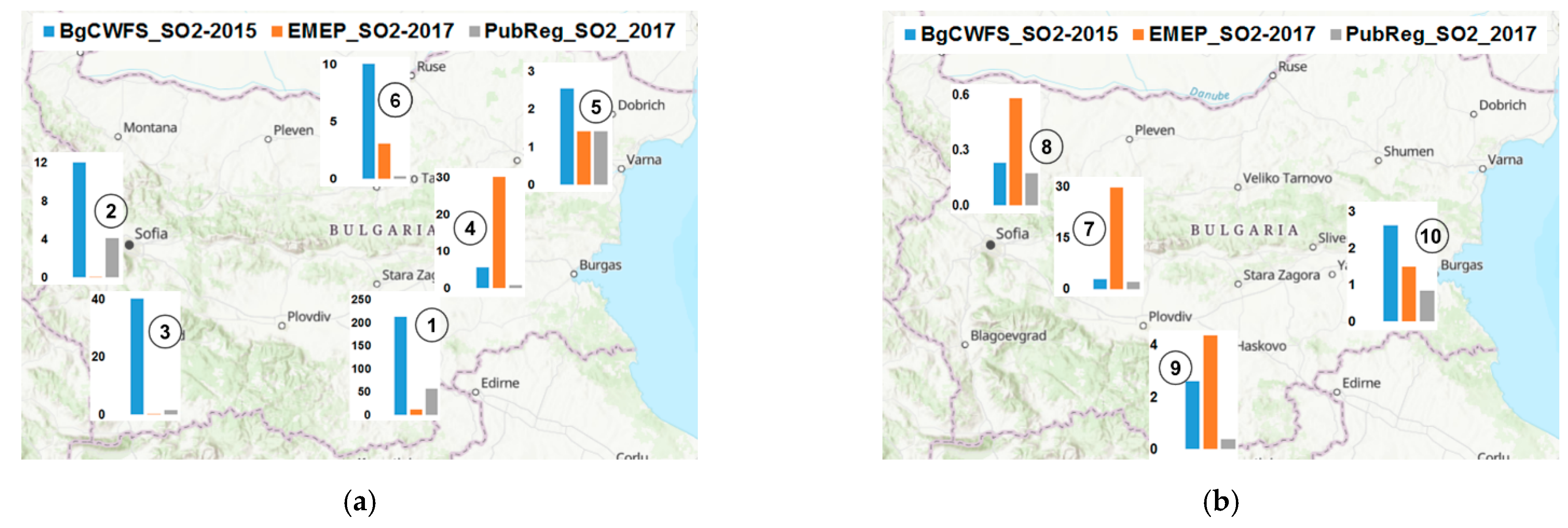
The distribution of the emission sources over the territory of the country (spatial allocation) is also important in air quality modeling. There were some notable differences, mainly for SOx source allocations, between the two models. The locations of the main SOx large point sources in Bulgaria (TPP and industrial facilities) are shown in Figure 1. The bars in Figure 1 indicate SOx emissions (kilotons per year) as used by the two models and as reported in the European Pollutant Release and Transfer Register (EPRTR) [51] for 2017. While BgCWFS overestimated the emissions from TPPs with site numbers 1–3, the EMEP-CTM model underestimated these emissions and overestimated largely the emissions at TPP site number 4 (Figure 1a). For the industrial facilities (Figure 1b) the main overestimation by EMEP-CTM compared to reported SOx emissions was for the plant for copper production and processing of metals “Aurubis” (site number 7), and for the plant KCM producing non-ferrous metals (site number 9). The SOx emissions for the facilities with site numbers 1 to 10 are listed in Table 2. The last column in Table 2 includes satellite derived SO2 emissions for the TPPs with site numbers 1 and 3 in 2017. They were extracted from the global catalogue of large SO2 emission sources based on the onboard Ozone Monitoring Instrument (OMI) [52,53]. It can be noticed that the EMEP-CTM model underestimated by a factor of 6 the emissions from the TPP complex “Maritsa East” (site number 1, south-east Bulgaria), which is one of the biggest coal-fired power stations on the Balkan Peninsula.
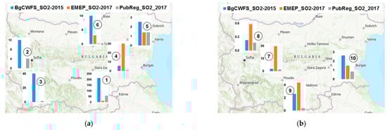
Figure 1.
Main sources of SOx emissions (kt.y-1) in Bulgaria: (a) TPPs; (b) industrial plants; BgCWFS (2015)—blue bars, EMEP-CTM (2017)—brown bars, EPRTR (for 2017)—grey bars. Site numbers corresponds to the names in Table 2.
Table 2.
SOx emissions (kt.y-1) from main point sources in Bulgaria from different sources: as used in the models (BgCWFS, EMEP), as provided by the EPRTR register [51], and as estimated based on retrievals of the satellite on-board OMI instrument [53]. TPP denotes coal-fired thermal power plants.
2.2. The Observational Data for Wet and Dry Depositions
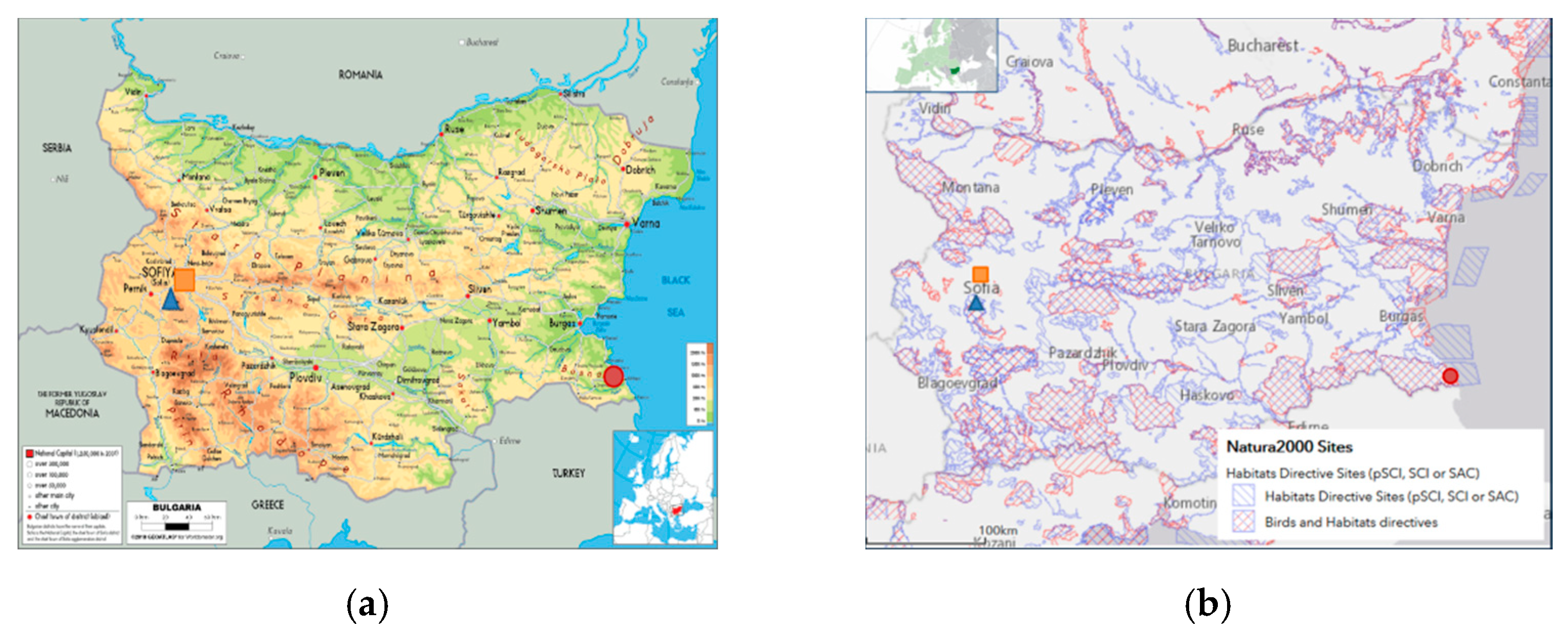
Field sampling campaigns for deposition samples and their chemical analysis were organized at three sites. The sites are located in different terrains (Figure 2) as follows: in a highly urbanized area, at the Central Meteorological Observatory of Sofia city (42.655° N, 23.384° E, 586 m above sea level (a.s.l.), in a mountain area, at the synoptic station Peak Cherni Vrah (42.616° N, 23.266° E, 2230 m a.s.l.), and in the Black Sea coastal area, at the synoptic station Ahtopol (42.084° N, 27.952° E, 26 m a.s.l.). Two of the stations, Cherni Vrah and Ahtopol are situated in nature protected areas (Figure 2b). The site in Ahtopol is near the coast, in an area part of the nature protected area Strandja, rich in flora and fauna species.
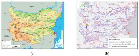
Figure 2.
Locations of the 3 sampling sites on: (a) topographic map of Bulgaria; (b) map of Bulgaria with nature protected areas (source: https://natura2000.eea.europa.eu/, accessed on 10 February 2021; orange square—Sofia, blue triangle—Cherni Vrah, red circle—Ahtopol.
Wet and dry depositions in Sofia and Ahtopol were sampled with an automatic wet only device (WADOS, Kroneis GmBH). The sampler contains a humidity sensor which controls the lid of wet and dry collector compartments automatically. During the wet deposition events, the sensor moves the lid onto the dry collector and after the sensor surface becomes dry, the lid on the dry collector goes onto the wet collector. Wet deposition samples were sampled on daily base (used for monthly estimates), while dry deposition samples were collected on a monthly basis in Sofia and Ahtopol. Deionized water was added into the bucket for dry deposition before sampling. A passive bulk sampler was operated at Cherni Vrah. After each sampling, the funnel was washed with deionized water.
All collected samples were further analyzed for acidity (pH), electro-conductivity (EC), main anions Cl−, SO42–, NO3− cation NH4+, and elements Ca, Mg, K, Na, Fe, Si, Zn, Cu. The chemical analysis was carried out with Ion Chromatograph (ICS 1100, DIONEX), ICPOES (Vista MPX CCD Simultaneous, VARIAN) and Spectrophotometer S-20.
In order to calculate the wet deposition of sulfur and nitrogen species, the measured concentration (mg·L−1) of each species (SO42–, NO3−, NH4+) was multiplied by the observed precipitation amount (L·m−2). The concentration of non-sea salt (non-marine) sulfate (nss_SO42−) was estimated by a correction based on the assumption that sodium is a sea salt tracer: [nss_SO42−] = [SO42−] − (0.25 × [Na]), following WMO recommendations [54]. In this work, data for the period from June to December 2017 were used.
2.3. Evaluation of Model Performance
The wet depositions as estimated by the two modeling systems were analyzed in two steps: model to model, and models to observations. The models were inter-compared on a quarterly and annual basis for the years 2016 and 2017, focusing on domain mean values (the average of the depositions for the grid nodes located in Bulgaria). The spatial distribution of S, RDN, and OXN wet and dry depositions was visualized on maps and compared qualitatively. The performance of the two models for precipitation was discussed in terms of annual domain mean and maximum values, quarterly domain mean values, and qualitative comparison of annual precipitation maps.
The comparison of modeled to observed depositions at the three sites was carried out for mean monthly values for the period from June to December 2017. Daily mean wet depositions at Cherni Vrah were analyzed only for three short-term periods, characterized by particular meteorological situations. The performance of the models for the selected periods was commented in view of mean values and normalized mean bias (NMB), where negative values indicate underestimation and positive values overestimation by the models.
3. Results
3.1. Wet Depositions Modeled by BgCWFS and EMEP-CTM
3.1.1. Precipitation
Wet deposition estimates depend strongly on the precipitation amounts. Thus, we comment firstly differences between the modeled precipitations. Figure 3 shows the spatial distribution of the annual accumulated precipitation in 2017 as simulated by BgCWFS with application of the precipitation bias adjustment (PBA) and by EMEP-CTM, and as constructed using observations. Both models provided higher precipitation amounts for the mountain areas. To note also that the models indicated elevated precipitation in the most south-eastern part of the country where the sampling site Ahtopol is located.
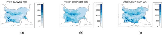
Figure 3.
Accumulated annual precipitation (mm) for 2017: (a) BgCWFS with PBA; (b) EMEP; (c) observed.
The domain mean annual precipitation, as estimated by observations, was higher in 2017 than in 2016 (Table 3). This was correctly simulated by BgCWFS, while EMEP-CTM provided almost identical domain mean precipitation amounts. BgCWFS overestimated the observed domain mean precipitation in 2017 by about 8%, while EMEP-CTM underestimated it by about 5%. A significant difference between the models was noted for the domain-wide maximum annual precipitation, as follows: BgCWFS results were with NMB of about −4%, while EMEP-CTM results were with NMB of about −29%.
Table 3.
Accumulated annual precipitation PR (mm) in Bulgaria in 2016 and 2017—observed and modeled, with domain mean values (mean) and domain maximum values (max).
The differences between the models on a quarterly basis (Table 4) indicate that BgCWFS simulated more precipitation than EMEP-CTM in the period from April to June (AMJ) and less precipitation in the period from July to September (JAS). Compared to observed precipitations, EMEP-CTM performed better with NMB from −2% to 9%, while the NMB for BgCWFS was from −23% to 25%.
Table 4.
Domain mean quarterly precipitation PR (mm) in Bulgaria in 2016 and 2017—observed and modeled; JFM (January, February, March), AMJ (April, May, June), JAS (July, August, September), OND (October, November, December).
3.1.2. Domain Mean Wet Depositions
Annual and quarterly S, OXN and RDN wet depositions (WD) simulated by the two models for 2016 and 2017 were compared as domain mean values, Table 5. Both models indicated prevalence of sulfur over nitrogen wet depositions. Annual values for S-WD by BgCWFS were higher by a factor of 1.5 than the ones by EMEP-CTM, most likely linked to the higher emissions used in BgCWFS. The annual values of RDN-WD and OXN-WD by BgCWFS were, however, lower than the EMEP-CTM values by about 12% and 28%, respectively. Both models simulated higher S-WD for the period from January to June, in correspondence to higher emissions and precipitations in this period. For the last three months of 2017 the S-WD by both models were relatively high, most likely due to the higher precipitation amounts by the models. For nitrogen depositions, the most significant difference was in the period from June to September, when EMEP-CTM values for RDN and OXN-WD were twice as high as the respective depositions by BgCWFS.
Table 5.
BgCWFS and EMEP-CTM wet depositions (mg·m−2) of sulfur (S), reduced (RDN) and oxidized nitrogen (OXN): domain mean values for Bulgaria, for period abbreviations see Table 4.
3.1.3. Spatial Distribution of Wet Depositions
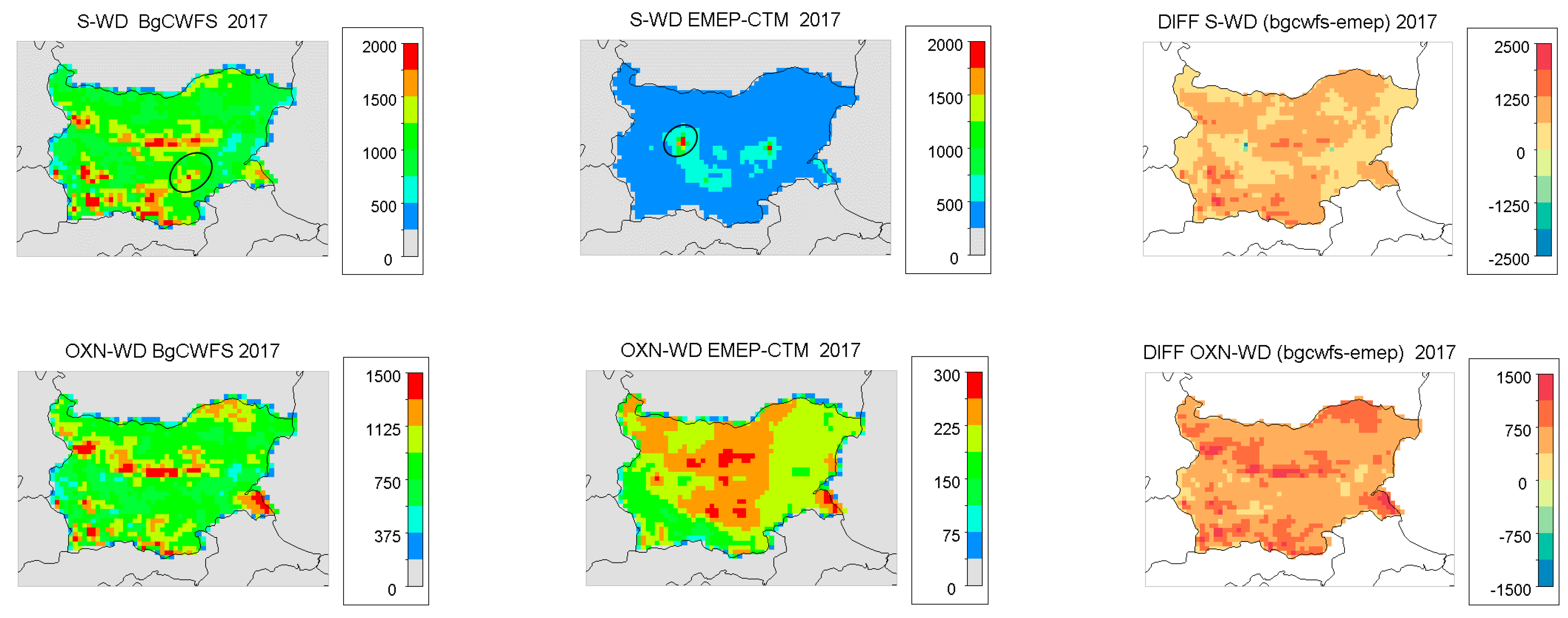
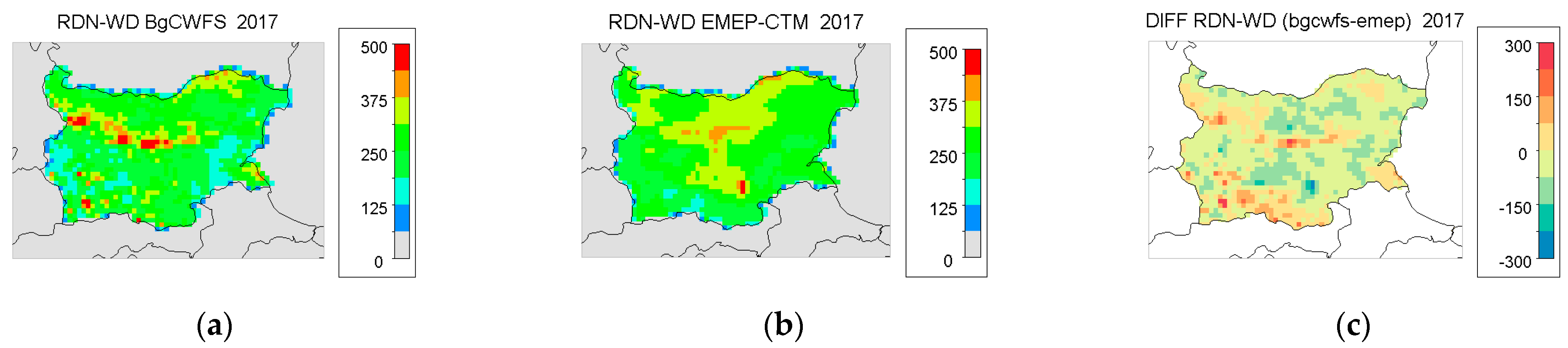
The spatial distribution of annual wet depositions in 2017 showed significant differences between the two models (Figure 4). In general, BgCWFS wet depositions were higher in regions with more precipitation (mountain areas), while EMEP-CTM wet depositions were higher near the emission sources used in this model. The maps for S-WD clearly indicated the difference in the locations of significant SOx emission sources: on the BgCWFS map this is TPP complex “Maritsa East”, while on the EMEP-CTM map this is the industrial plant “Aurubis”. As discussed in Section 2.1.2, EMEP-CTM had short-comings in the SOx emission quantities for these two facilities—the fingerprint of the first one is invisible on the EMEP-CTM maps, while the second one appears as a hot-spot. The maps for the differences between BgCWFS and EMEP-CTM wet depositions (Figure 4c) showed that S-WD and RDN-WD by BgCWFS were higher than the ones by EMEP-CTM over the whole country, while for OXN-WD the opposite was true. Bigger urban areas were noticed as hot spots of OXN-WD on the EMEP-CTM map, while such urban hot-spots were missing on the BgCWFS map. This suggested a deficit in NO2 emissions input in BgCWFS.

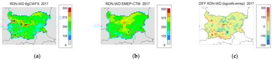
Figure 4.
Wet depositions (mg·m−2) for 2017: (a) BgCWFS; (b) EMEP-CTM; (c) differences (BgCWFS−EMEP-CTM); top panels S-WD, middle panels OXN-WD (note different scales), bottom panels RDN-WD; circle on S-WD map in column (a) indicates the TPP “Maritsa East”, circle on map S-WD in column (b) indicates the industrial plant “Aurubis”.
For the most south-eastern part of the country, characterized by numerous protected areas of nature, both models indicated higher values of S-WD and OXN-WD.
The maps for 2016 (not shown here) had similar patterns.
3.2. Dry Depositions of Sulfur, Reduced Nitrogen and Oxidized Nitrogen
3.2.1. Domain Mean Dry Depositions
Table 6 shows domain mean values of annual and quarterly depositions of S, OXN and RDN dry depositions (DD) simulated by the two models for 2016 and 2017. The S-DD by BgCWFS were higher by a factor of 6–7 than the S-DD by EMEP-CTM, reflecting the bigger SOx emissions used in BgCWFS. The variability for S-DD was much higher in BgCWFS values than in EMEP-CTM. As for wet depositions, BgCWFS estimated prevalence of sulfur dry depositions over nitrogen dry depositions. On a contrary, S-DD values by EMEP-CTM were similar to RDN-DD and OXN-DD. On an annual basis, EMEP-CTM simulated OXN-DD higher than S-DD and RDN-DD by about 12%. The OXN-DD by BgCWFS were about 30% lower than the ones by EMEP-CTM, pointing to shortcomings in NOx emissions used in BgCWFS.
Table 6.
BgCWFS and EMEP-CTM dry depositions of sulfur (S), reduced (RDN) and oxidized nitrogen (OXN): domain mean values for Bulgaria, for period abbreviations see Table 4.
3.2.2. Spatial Distribution of Dry Depositions
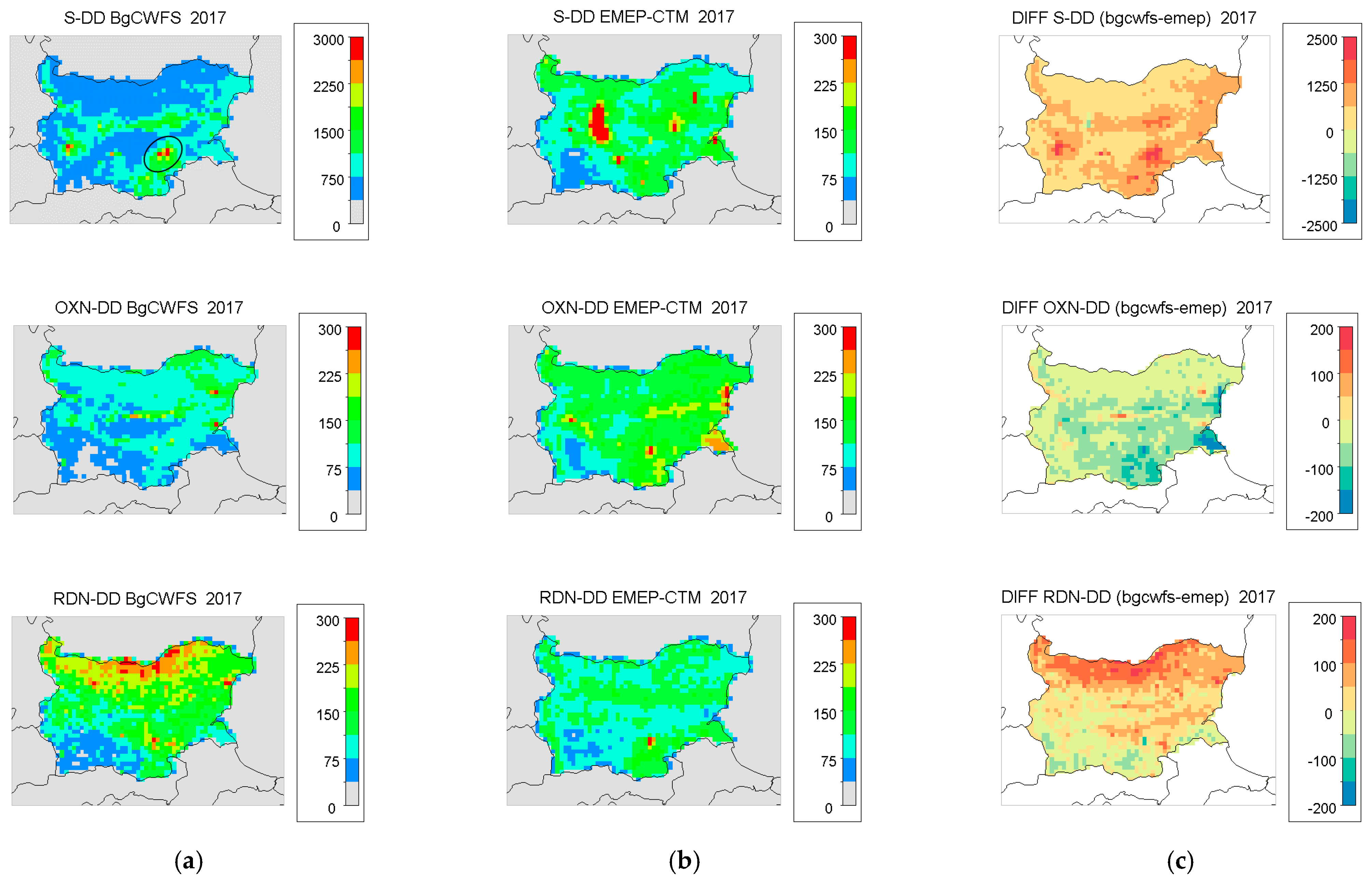
The spatial distribution of modeled dry depositions depends mainly on the location of the sources. As both models exploited different emission inventories, significant differences were noted in the corresponding maps (Figure 5). BgCWFS represented better the position of the national source with highest SOx emissions—the TPP complex “Maritsa East” in the southern part of the country (marked by circle in Figure 5). The map for the differences in S-DD indicated that BgCWFS provided much higher values than EMEP-CTM over almost the whole country. For OXN-DD, both models simulated higher values in the eastern part of the country, where coastal big cities were better evident on the EMEP-CTM map. The main differences in the spatial pattern for RDN-DD were in the northern part of the country, where BgCWFS values were higher by a factor of two.
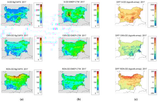
Figure 5.
Dry depositions (mg·m−2) for 2017: (a) BgCWFS; (b) EMEP-CTM; (c) differences (BgCWFS—EMEP-CTM); top panels S-DD (note different scales), middle panels OXN-DD, bottom panels RDN-DD; circle on S-DD map in column (a) indicates the TPP “Maritsa East”.
3.3. Total Depositions of Sulfur, Reduced Nitrogen and Oxidized Nitrogen
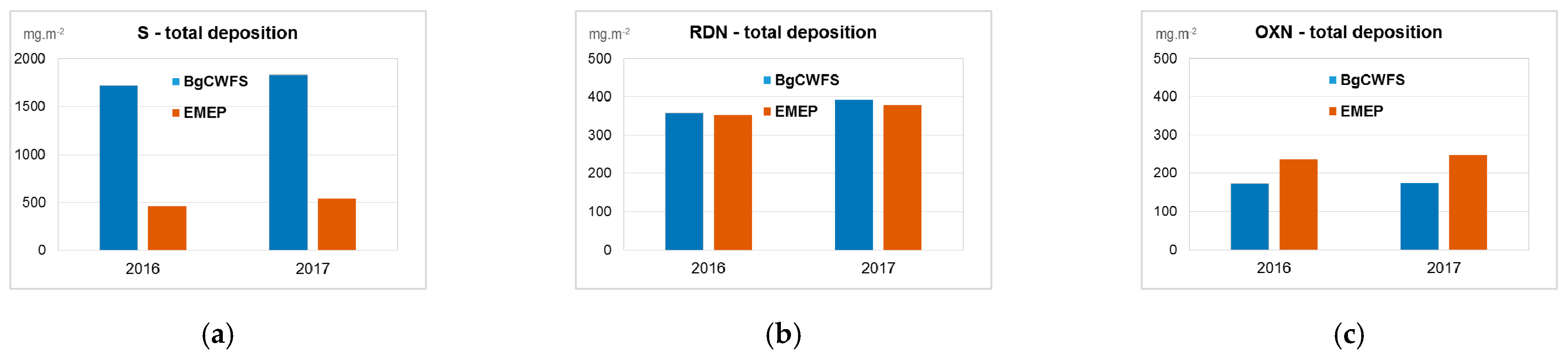
The total (wet plus dry) depositions for domain mean annual values estimated by BgCWFS and EMEP-CTM models are presented in Figure 6. Sulfur total depositions were higher than the reduced nitrogen and the total oxidized nitrogen depositions for both models. The most significant difference between the models was for sulfur deposition, e.g., the domain mean total S deposition by BgCWFS was higher than the one by EMEP-CTM by a factor of about 3.5. For reduced nitrogen depositions, both models provided similar values, while for total oxidized nitrogen deposition the difference showed lower BgCWFS values by about 28%. A difference between the models was noted when comparing sulfur total depositions with total nitrogen depositions (reduced plus oxidized). BgCWFS indicated a notable prevalence of sulfur over nitrogen depositions, while EMEP-CTM suggested a prevalence of nitrogen deposition over sulfur deposition, by about 21% in 2016 and 14% in 2017.
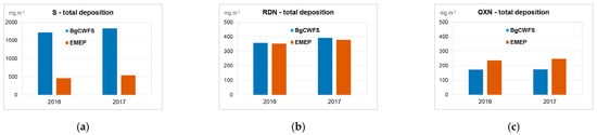
Figure 6.
Total depositions (mg·m−2)—domain mean values by BgCWFS and EMEP-CTM for 2016 and 2017: (a) sulfur; (b) reduced nitrogen; (c) oxidized nitrogen.
3.4. Comparison to Observed Depositions at Sampling Sites
3.4.1. Chemical Analysis of Precipitation Samples
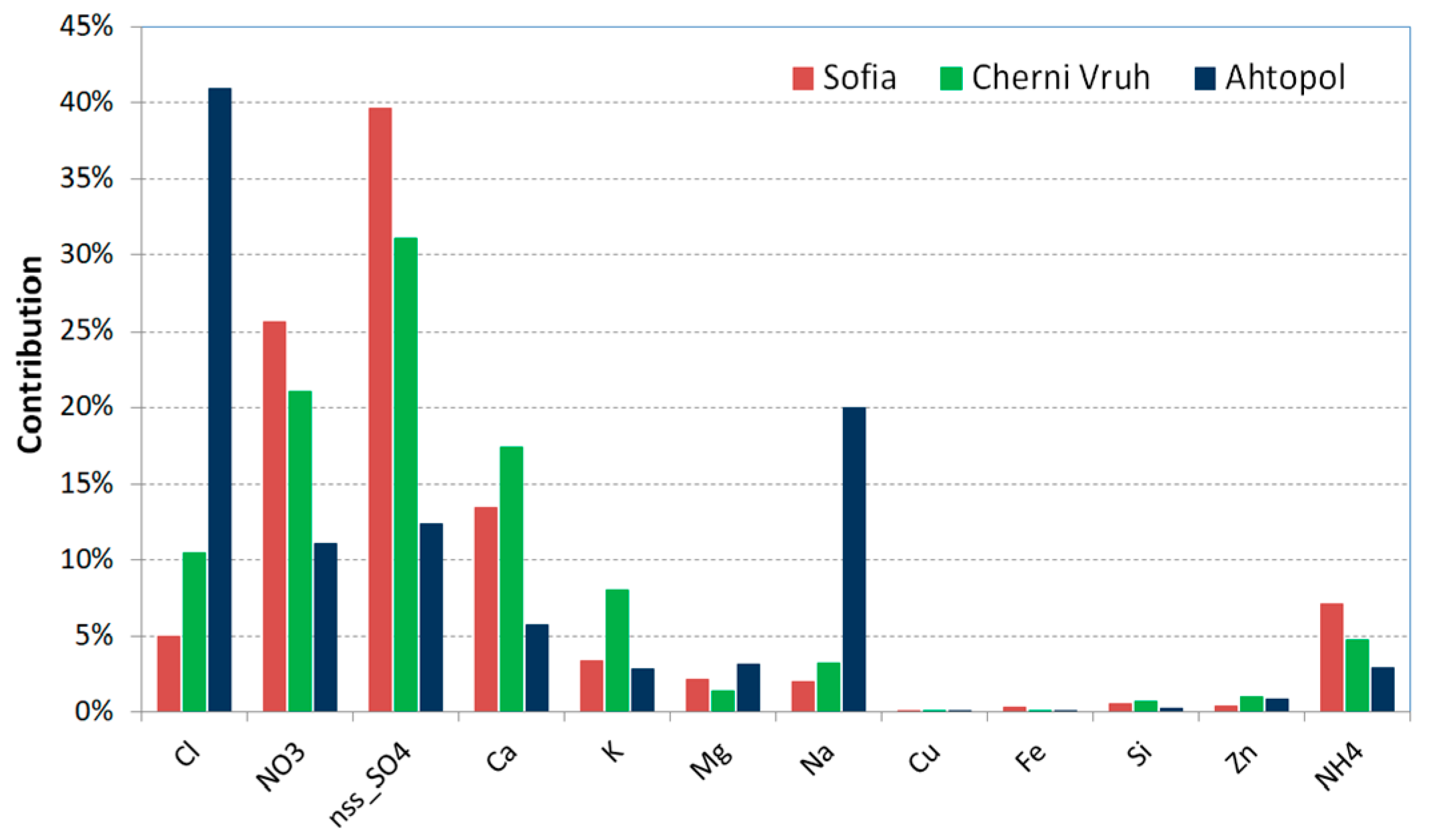
The percentage contribution of ions and elements to the total mass of all analyzed species in precipitation samples for the period from June to December 2017 are presented in Figure 7. The mean concentrations of all elements were generally higher for the mountain site. An exception was noticed for the coastal site Ahtopol where concentrations of Cl and Na were higher than for the other sites. Generally, nss_SO42– was found to be the dominant anion in precipitation samples from Sofia and Cherni Vrah (39.6% and 31.2%, respectively), followed by NO3− (21.6% and 25.6%, respectively) and Cl− (4.9% and 10.4%, respectively). At the coastal site Ahtopol, the Cl anion showed a higher contribution (41%), as was expected for a site near the sea, followed by nss_SO42– (12.3%) and NO3− (11.1%). The contribution of sea/marine aerosol to the total concentration of sulfates was also high for samples from Ahtopol. On average for Ahtopol, the sea salt sulfate contribution in wet deposition samples was 22%, and in dry deposition samples it was 18%. These values were much higher than for Sofia and Cherni Vrah, where in wet deposition samples the sea salt sulfate contribution was only about 1% of the total sulfate concentrations.
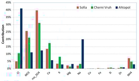
Figure 7.
Percentage contribution of different elements in precipitation samples at 3 sites (indicated by color) for the period June–December 2017.
The predominant cation for Sofia and Cherni Vrah was Ca representing, with a share of, respectively, 13.4% and 17.4%, while for Ahtopol the predominant cation was Na (19.9%). The share of ammonium ions was highest for Sofia (7.12%), for Cherni Vrah it was 4.75%, and for Ahtopol it was 2.9%.
The percentage contribution of different elements in the precipitation samples for all sites was in the following order:
Sofia: nss_SO42– > NO3− > Ca > NH4+ > K > Cl > Na > Mg > Si > Fe > Zn > Cu,
Cherni Vrah: nss_SO42– > NO3− > Ca > Cl > K > NH4+ > Na > Mg > Zn > Si > Fe > Cu,
Ahtopol: Cl > Na > nss_SO42– > NO3− > Ca > Mg > NH4+ > K > Zn > Si > Fe > Cu.
3.4.2. Comparison to Wet Depositions at Three Sites
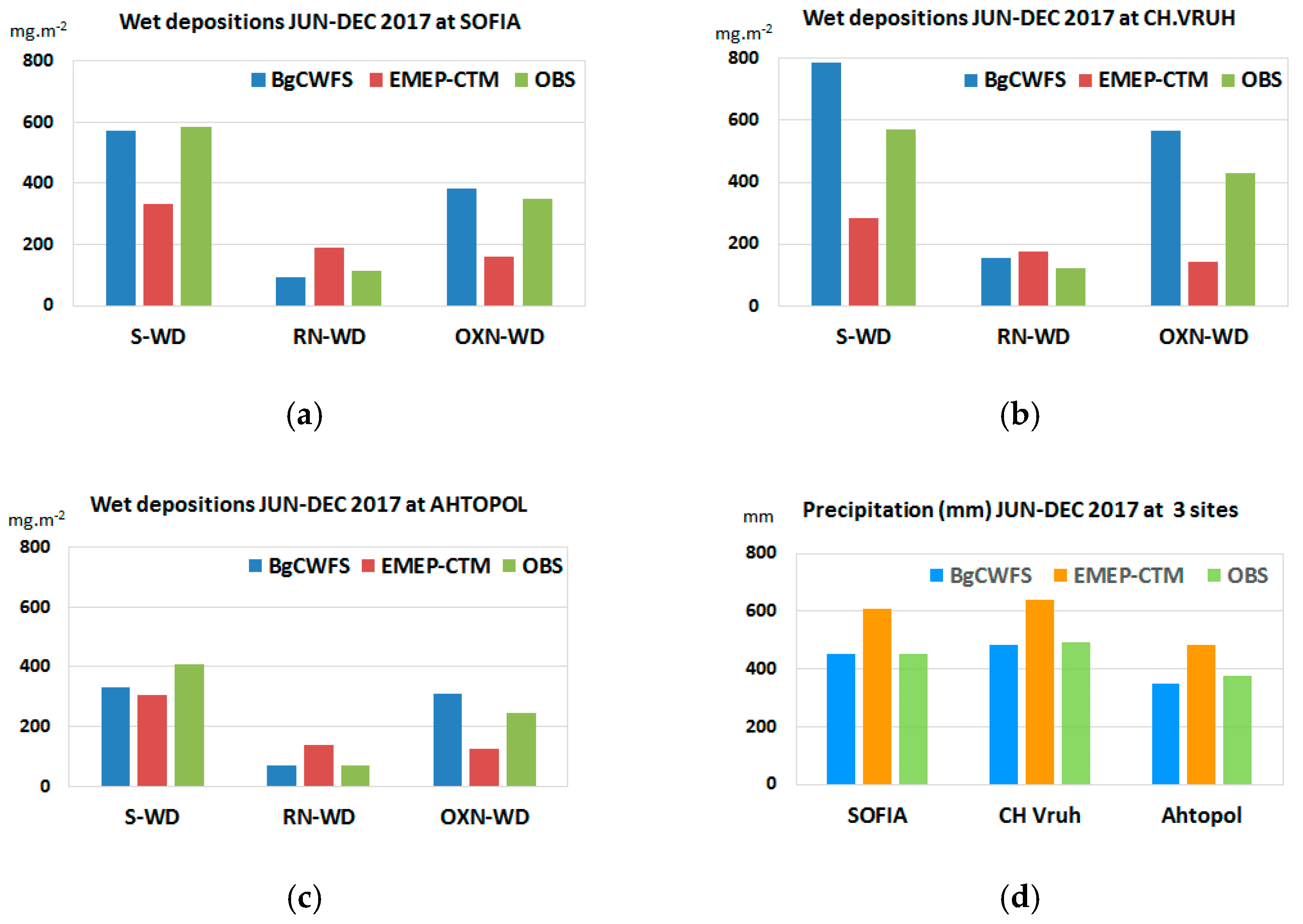
The comparison for S, RDN and OXN wet depositions was carried out on monthly basis for the period from June to December 2017 at all three stations. Hereafter, the observed S-deposition is corrected for sea salt contribution. Both models correctly simulated high S-WD at the three sites (Figure 8). However, EMEP-CTM significantly underestimated S-WD at two of the sites. The absolute value of the mean NMB was about 15% for BgCWFS (with overestimation for Cherni Vrah), and about 43% for EMEP-CTM (with underestimation at all sites). In another study, based on comparison of EMEP-CTM to data from the EMEP monitoring network in 2017 [55], an underestimation of sulfur depositions was also reported, to the value of about 27% on average. The analysis in [55] further showed EMEP-CTM model results for OXN-WD without significant bias with respect to observations, while the RDN-WD were overestimated by 17%. For the period investigated in this work, the EMEP-CTM wet depositions at the three stations were characterized also by underestimation for S-WD (varying from 28% to 54%), an overestimation for RDN-WD (varying from 59% to 98%), and underestimation for OXN-WD, (varying from 51% to 69%). These higher biases with respect to the ones reported in [55] were partly due to the shorter period of analysis in this study.
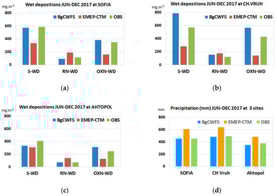
Figure 8.
Comparison of wet depositions (mg·m−2) for: (a) Sofia; (b) Cherni Vrah; (c) Ahtopol; and (d) comparison of precipitation (mm) at the 3 sites, for the period—June to December 2017.
Figure 8 indicates that BgCWFS performs, in general, better than EMEP-CTM at the sampling sites, despite the usage of outdated emissions. The accumulated precipitation amount by EMEP-CTM is higher than the observed one for the studied period (Figure 8d). This suggests that the better agreement of BgCWFS results to observed wet depositions might be linked to better allocation of the main national emission sources. The significant underestimation of S-WD at stations Sofia and Cherni Vrah by EMEP-CTM is most probably due to underestimation of emissions from the large emission sources in the western part of the country, as shown in Figure 1.
3.4.3. Comparison to Dry Depositions at Two Sites
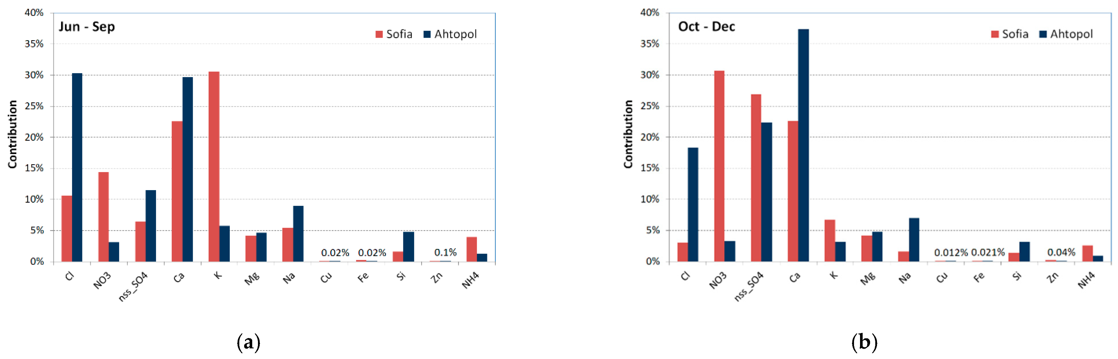
The percentage contribution of ions and elements to the total mass of all analyzed species in dry deposition samples for the periods from June to September, and from October to December 2017 is presented in Figure 9.
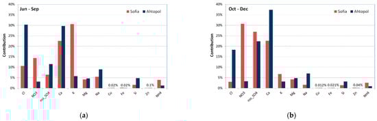
Figure 9.
Percentage contribution of different elements in dry deposition samples from Sofia (red color) and Ahtopol (dark blue color) for the period: (a) June–September 2017; (b) October–December 2017.
For Sofia, the contributions of NO3− and nss_SO42− were higher in the colder period (October to December) with a share of 30.7% and 27%, respectively, in comparison to 14.4% and 6.4%, respectively, in the warmer period (June to September). The contributions of Cl, Na, K, NH4+ were also higher in the colder period (10.6%, 5.4%, 30.5%, 4%, respectively) than the shares in the warmer period (3%, 1.6%, 6.7%, 2.6%, respectively,). For Ahtopol, the contributions of Cl and Na were higher in the warmer period (30.3% and 9%, respectively) than in the colder period (18.4% and 7%, respectively). The nss_SO42− contribution in the warmer period (11.5%) was lower than for the colder period (22.4%). The contribution of NO3− (3%) in Ahtopol for both periods was much smaller than in Sofia.
For the whole period from June to December 2017, the dominant anion for Sofia was NO3− (18%), followed by nss_SO42– (12.5%) and Cl− (9.8%). For Ahtopol, the dominant anion was Cl− (24.8%), followed by nss_SO42– (16.8%) and NO3− (3%). There was a notable share of the crustal elements Ca and K in the samples from Sofia. For both sites, the predominant cation in dry deposition samples was Ca, with a share of 23.6% and 33.6%, respectively. The share of ammonium ions was higher for Sofia (3.4%) than for Ahtopol (1.1%).
The percentage contribution of different elements in the dry deposition samples for Sofia and Ahtopol for the period from June to December 2017 was in the following order:
Sofia: Ca > K > NO3− > nss_SO42– > Cl > Na > Mg > NH4+ > Si > Fe > Zn > Cu,
Ahtopol:Ca > Cl > nss_SO42– > Na > Mg > K > Si > NO3− > NH4+ > Zn > Fe > Cu.
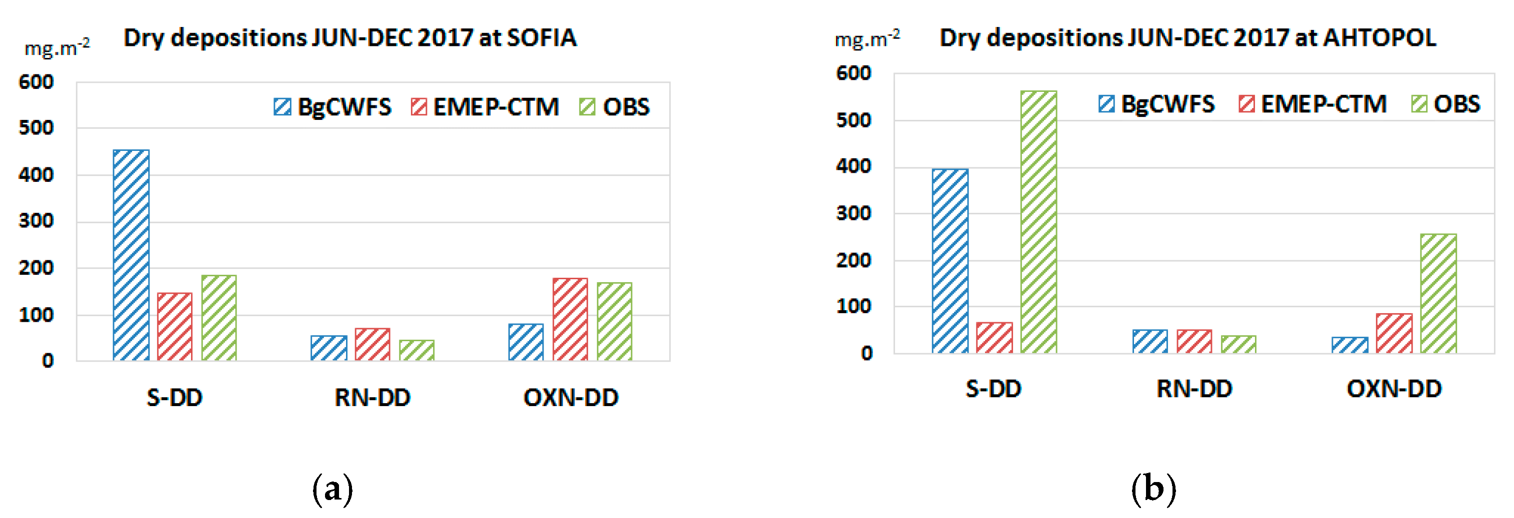
The comparison between model and observed dry depositions accumulated in the period June–December 2017 (Figure 10) shows that BgCWFS largely overestimated S-DD in Sofia, and underestimated S-DD in Ahtopol, while EMEP-CTM significantly underestimated S-DD in Ahtopol. The underestimation of the S-DD in Ahtopol by both models was most probably linked to the resolution of the models, limiting the representation of local circulations in this complex coastal area. Another cause might be related to local emission sources—e.g., intensive road traffic in summer and wood burning from residential heating in autumn—not accounted for in the model for the studied period.
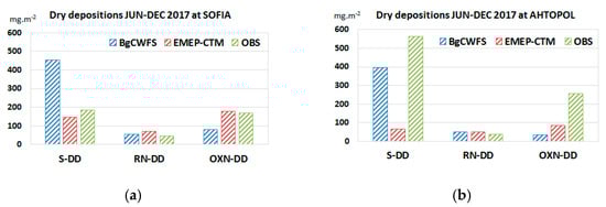
Figure 10.
Comparison of dry depositions (mg·m−2) by BgCWFS, EMEP-CTM and observations for: (a) Sofia; (b) Ahtopol; period June–December 2017.
The observed S-DD at the coastal site Ahtopol were higher than in Sofia. One of the reasons for this was the difference in the amount of accumulated precipitations for the studied period, with values at Ahtopol lower by more than 20% compared to values in Sofia. The number of days with precipitation in Ahtopol was also less (16) than in Sofia (25), suggesting that the removal of pollutants in Sofia was mainly through the wet deposition. Higher dry depositions of sulfur in Ahtopol in summer months (June to August) could be linked also to influence from the industrial plant “Lukoil Neftochim” Burgas, the largest refinery in the Balkans, located at about 60 km northwards. The SO2 concentration observed in Burgas at the background urban station BG0056 “Meden Rudnik” (not far away from the refinery plant “Lukoil Neftochim”) had a mean value of 8.90 µg·m−3 for the studied period. At the same time, the mean SO2 concentration in Sofia, observed at the background urban site BG0079 Sofia “Mladost” in the vicinity of the sampling site, was significantly lower (3.12 µg·m−3). The prevailing synoptic flow along the Bulgarian Black Sea coast might have contributed to higher dry depositions in Ahtopol. During the months of July and August, the prevailing winds at the southern Bulgarian Black Sea coast are from N to NE, the so called Etesian winds [56]. These rather intense winds contribute to higher turbulence and enhance the dry deposition of pollutants. The second half of the period (September to December) was characterized by more frequent passages of atmospheric perturbations from NW and SW, also reaching the coastal area. Thus, higher dry depositions in Ahtopol for the period June to December could be linked to influence from both national emission sources and sources outside of the country.
3.5. Effects of Long Range Transport on Depositions at Mountain Site Cherni Vrah
A combined analysis of back-trajectories and data from the chemical analysis of precipitation samples collected at the high mountain site Cherni Vrah was carried out aiming to identify the effects of long-range transport on precipitation chemical composition.
We briefly discuss three periods of 2017 characterized by elevated values of sulfate and nitrate concentrations in the samples: 16–17 June, 12–13 August and 26–28 September. Back-trajectories were calculated at three heights above ground level (500 m, 1000 m, and 2000 m) using the model HYSPLIT [57,58].
The wet depositions of sulfur, reduced nitrogen and oxidized nitrogen were estimated from the two models, BgCWFS and EMEP-CTM, and also based on the chemical analysis of the wet samples (observations). Then, the NMB was calculated for each model and each period.
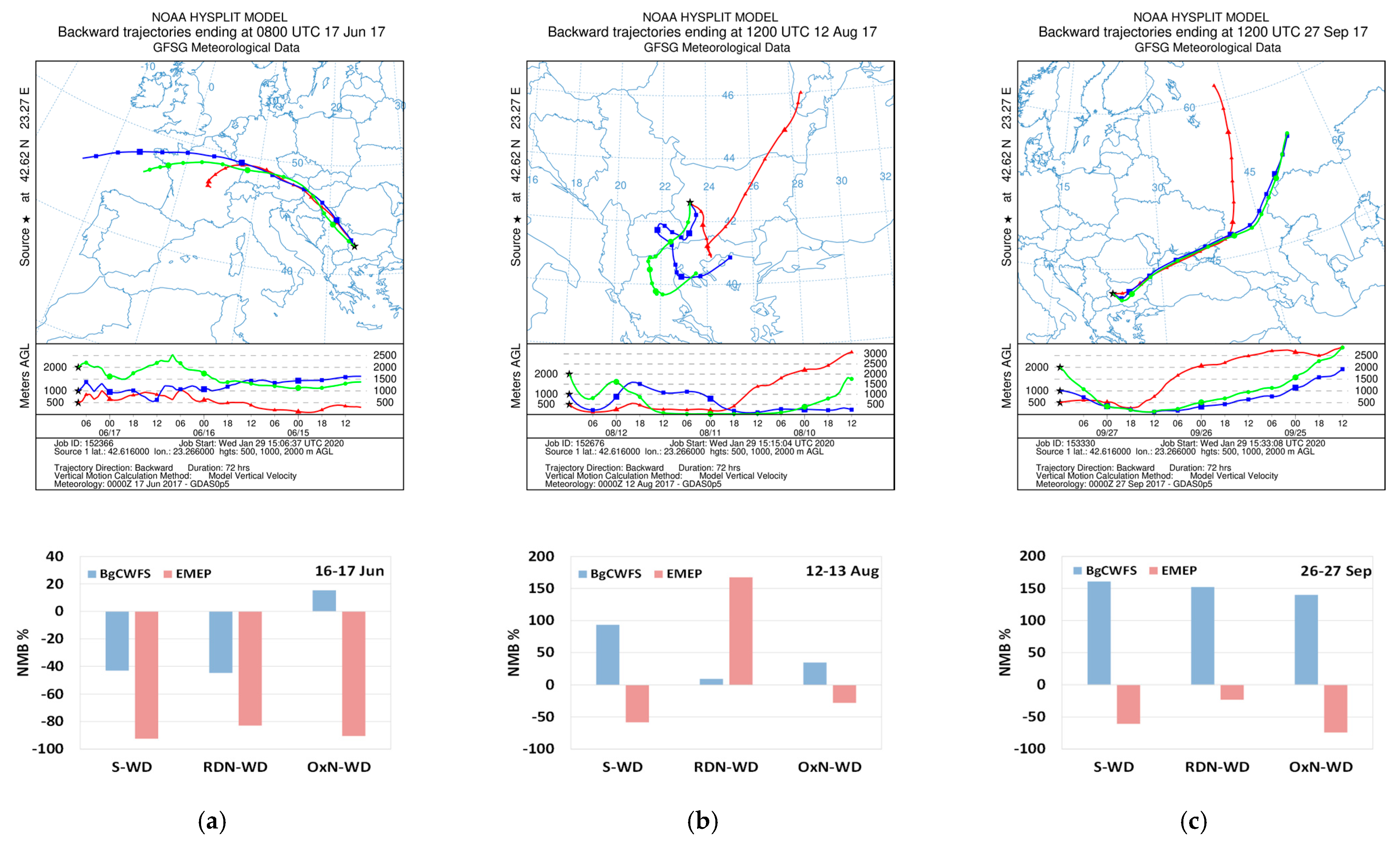
Figure 11 shows the pathway of the air masses and the NMB for BgCWFS and EMEP-CTM for the three cases. In the first period, the synoptic situation was characterized by the passage of a fast cold front from NW with light to moderate precipitations in the western part of the country. North-westerly outbreaks are typical for the western part of the country, where both Cherni Vrah and Sofia are located. In such types of outbreaks, the wet depositions of sulfur prevail over wet depositions of nitrogen [29]. For the two days 16–17 June, the non-sea salt sulfur deposition was 36.1 mg·m−2, and the total nitrogen deposition was 31.2 mg·m−2, as estimated based on observations. Both models simulated correctly the prevalence of S-WD over N-WD, but underestimated S-WD and RDN-WD. The NMB for depositions by BgCWFS was lower (Figure 11a), likely due to lower bias in precipitation (−35% compared to −70% by EMEP-CTM). The pathway suggests influence from TPPs located north-west of the country. The second period is typical for August in Bulgaria when anticyclonic weather conditions prevail, and the precipitations are often associated with local phenomena or the passage of low-pressure systems southward of the country. In this case, both models overestimated the precipitation by a factor of 2–3, but the NMB by the models for different types of deposition was variable (Figure 11b), suggesting higher impact by emission sources. The chemical composition showed relatively high amount of K (0.46 mg·L−1), likely due to influence from forest fires in the western part of the Balkans. Satellite images (https://firms.modaps.eosdis.nasa.gov/, accessed on 10 February 2021) indicated numerous forest fires south-west of the country in the period 09–13 August. The third period was characterized also by easterly winds (Figure 11c). The chemical analysis of the precipitation sample showed elevated concentrations of Cu (on average 0.014 mg·L−1), most likely due to influence from the Aurubis copper smelter plant located eastward of the sampling site (site number 7 in Figure 1). The precipitation was underestimated by both models; however, the NMB for the depositions were of opposite signs by the two models, with a better score for EMEP-CTM.
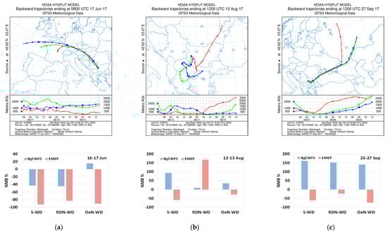
Figure 11.
HYSPLIT back-trajectories (top panels) and NMB (%) (bottom panels) in wet depositions by BgCWFS and EMEP-CTM for 3 selected periods: (a) 16–17. June 2017; (b) 12–13 August 2017; and (c) 26–27 September 2017; blue bars refer to BgCWFS, red bars refer to EMEP-CTM.
4. Discussion
Results from two modeling systems (BgCWFS, based on WRF-CMAQ, and EMEP-MSC-W rv4.33) were compared for wet and dry depositions of sulfur, reduced nitrogen and oxidized nitrogen for the territory of Bulgaria in 2016 and 2017. The models have similar grid resolutions (about 10 km), but different inputs and parameterization schemes. Significant differences were noted in the emission input, as follows: in BgCWFS, the emissions were for the year 2015 at national level, and for 2011 for the European domain, while EMEP-CTM exploited up-to-date emissions for the years 2016 and 2017. The analysis of SOx emissions used by the two models and their comparison to data from the European Pollutant Release and Transfer Register for the year 2017 showed short-comings in EMEP-CTM relevant to the locations and intensity of the main point sources in Bulgaria. For example, annual emissions from the coal-fired thermal power plant complex “Maritsa-East” in south Bulgaria were very low with respect to the officially reported data. This complex remains one of the major SOx polluters in the Balkans, despite the reduction in emissions in recent years, and it is important to be accurately represented in gridded emissions. EMEP-CTM undergoes annual validation based on observations from the EMEP monitoring sites for precipitation chemistry, which are not available in Bulgaria. This might have contributed to the undetected problems with emissions allocation in the country. The differences in the emission input led to different values of depositions, both in magnitude and in terms of spatial distribution. The outdated emissions in BgCWFS resulted in higher depositions especially for sulfur dry and wet depositions. Domain-averaged annual total depositions of sulfur estimated by BgCWFS were, by a factor of 3.5, higher than the ones simulated by EMEP-CTM. Another significant difference was noted for the total deposition of oxidized nitrogen, in that the domain-averaged value by BgCWFS was 28% lower than the one by EMEP-CTM. Only for reduced nitrogen wet depositions did both models provide similar domain-averaged values. The maps for the spatial distributions revealed significant differences in the footprint of the biggest emitters of pollutants at national scale (e.g., TPP complex “Maritsa East”).
Despite the differences in the results from the two systems, the model methodologies revealed some common features. Firstly, sulfur deposition in Bulgaria in 2016 and 2017 was higher than the depositions of reduced nitrogen and of oxidized nitrogen. Secondly, the most south-eastern part of the country was subject to both elevated S-WD and wet and dry OXN depositions. This could be related to effects of transboundary pollution. According to the country report by EMEP for 2017, the transboundary contribution to oxidized sulfur deposition and oxidized nitrogen deposition is about 80% for the south-eastern part of Bulgaria [26]. As this region has numerous protected areas of nature, further studies are necessary to investigate the depositions’ variability and the possible causes, taking into account effects both from national sources and from transboundary pollutant transport.
Prevailing sulfur depositions (wet plus dry) over the Balkans were also reported in the literature. In [24], based on model simulations for the period 2000–2007, the multi-year averaged S depositions in winter were more than 40% higher than the S deposition in summer. In our study, BgCWFS results averaged for 2016–2017 showed total S depositions for the period from January to March as being about 33% higher than for the period from June to September. This variability is linked to the intensity of the emissions sources in the region, where numerous coal-fired TPPs are operating. Additionally, in [15], the Balkans were identified as hot spots for S total depositions based on modeling results from 14 different CTMs for 2010. The trend of decreasing sulfur depositions in Europe in the period 1990–2010 was reported to be more pronounced before 2000, as a consequence of emission reduction strategies in Europe [14]. SOx emissions in Europe decreased by more than 80% during 2000–2019, but the observations in this period indicated an average reduction of 60% for sulfur wet deposition and that there were still many hot spots in South-East Europe [5]. The spatial distribution of depositions in Bulgaria for the period (2008–2014), discussed in [59], showed some similarities to the results in this work. In [59], the same CTMs were applied, but with different inputs. Similar to our results, the highest differences between the models in [59] was for sulfur deposition, both as magnitude and spatial distribution, indicating the importance of the SOx emission input to the models.
The chemical analysis of wet and dry atmospheric samples collected during June–December 2017 at three sites in Bulgaria showed prevalence of sulfate in the western part of the country, and Cl and Na at the coastal site Ahtopol. The sea salt contribution was also high at this site, with a share of 22% in wet precipitation samples and 18% in dry samples. The observed sulfur depositions (wet and dry) at all sites was higher than the oxidized and the reduced nitrogen depositions. Interestingly, the observed sulfur dry deposition at the coastal site was higher than the one in Sofia. Most likely this is due to the combined effect of local/regional circulations leading to more windy conditions, and influence from national and transboundary emission sources. A high share of sulfate and chlorine in wet samples at the south-eastern Bulgarian coast was also found in a previous study [30]. For the summer and autumn period of 2014, the predominant elements in wet samples from Ahtopol and Burgas were chlorine and sulphate, 39% and 19.5%, respectively. The analysis in [30] pointed out the effects of cyclone paths on the chemical composition of precipitation samples, showing that non-sea salt sulfate contribution increases for cyclones approaching the south-eastern part of Bulgaria from southern directions. The reported data for the observed dry deposition in Ahtopol in this work was in line with another study for the same site [60]. For July and August of 2018, the observed S dry deposition at Ahtopol was also higher than OXN-DD and RDN-DD, and the share of sea salt sulfate was 16% on average for the two months [60].
The collection of atmospheric samples at the three sites in Bulgaria (urban, mountain and coastal) does not have regular character, as they are carried out during experimental campaigns. The chemical analysis of these samples and the estimation of deposition, however, provide valuable background for the validation of modeling results in this part of South-East Europe, with a lack of precipitation chemistry data and dry deposition data.
The comparison of modeled to observed depositions showed that both BgCWFS and EMEP-CTM captured the prevalence of sulfur wet depositions in the period from June to December 2017 at all sites. S wet deposition by BgCWFS was with lower NMB (15%) compared to NMB by EMEP-CTM (58%) (NMB in absolute values). One possible reason for this better score of BgCWFS is the correct representation of the locations of national emission sources. The sulfur dry deposition at the coastal site Ahtopol was largely underestimated by both models (on average by more than 50%). In [60], results for S-DD at Ahtopol for the months from June to August of 2018 pointed to underestimation by EMEP-CTM of about 43%. Additional analysis with finer scale models suitable to represent the complex local circulations at these sites might be needed to have a more in depth insight for the depositions in this part of the country.
Variability in model results for depositions was reported by European wide model-intercomparison exercises [14,15]. Differences among the models are not surprising as they use different inputs and process parameterizations, and even a single model could provide different results due to different model versions. The differences between BgCWFS and EMEP-CTM depositions with reference to observations at three sites in Bulgaria were within the range reported in [14,15]. For S-WD, the NMB was between −51% and +38%, lower than the reported range in [14] (−70% to +82%). For RDN-WD, the NMB was in the range from −17% to +119%, compared to the one in [14] (−58%, +21%). For OXN-WD, the NMW was in the range from −67% to +32% within the range reported one in [14] (−86%, +72%). The results presented here for dry depositions showed a difference between model results by a factor of 2–3 for S-DD and OXN-DD and more agreement for the modeled RDN-DD, in line with the results discussed in [14].
5. Conclusions
We presented results for depositions in Bulgaria as estimated by two models: BgCWFS (the operational chemical weather forecasting system in Bulgaria) and EMEP-MSC-W rv3.33 (the model used for annual reporting on transboundary fluxes of particulate matter, photo-oxidants, acidifying and eutrophying components in Europe). The horizontal resolution of both models was similar (about 10 km), but emissions input, meteorological drivers and parameterization schemes were different. As a consequence, the spatial distribution of sulfur, reduced nitrogen and oxidized nitrogen had different patterns. However, some common features were noted as follows: both systems estimated sulfur depositions to be prevailing, with hot spots corresponding to big emission sources (coal-fired TPP or industrial facilities). Both models also indicated higher sulfur and oxidized nitrogen deposition in the most south-eastern part of the country—a region without significant emission sources and with numerous protected areas of nature. The variability of the modeled depositions was in agreement with findings from other studies for the Balkans and from well-known model-intercomparison exercises in Europe. The comparison of the model depositions to observed depositions at three sites in the country pointed out to some shortcomings in the models. For the region of the Balkans, where routine measurements of precipitation chemistry or dry deposition are missing, the data discussed here, though limited in time and space, provide the possibility to test model performance and thus contribute to the improvement of the models’ applications.
Author Contributions
Conceptualization, E.G. and D.S.; methodology, D.S., E.G. and E.H.; software, D.S., M.P. and I.G.; validation, E.G. and E.H.; formal analysis, all authors; investigation, all authors; resources, D.S. and E.H.; data curation, E.G., D.S. and E.H.; writing—original draft preparation, E.G.; writing—review and editing, B.V. and I.G.; visualization, E.G. and E.H. All authors have read and agreed to the published version of the manuscript.
Funding
This research was funded by the Bulgarian National Science Fund trough contract number DN-04/4-15.12.2016.
Institutional Review Board Statement
Not applicable.
Informed Consent Statement
Not applicable.
Data Availability Statement
All relevant data are reported in the paper.
Acknowledgments
The authors are grateful to US EPA for providing WRF-CMAQ models, to TNO for the emission inventory at European scale, to US NCEP for providing free-of-charge meteorological data, and to the NOAA Air Resources Laboratory (ARL) for the provision of the HYSPLIT model and READY website (http://www.ready.noaa.gov, accessed on 10 February 2021. Deep gratitude is due to the Norwegian Meteorological Institute (Met Norway) for the open access data from EMEP-MSC-W.
Conflicts of Interest
The authors declare no conflict of interest. The funders had no role in the design of the study; in the collection, analyses, or interpretation of data; in the writing of the manuscript, or in the decision to publish the results.
References
- Vet, R.; Artz, R.S.; Carou, S.; Shawa, M.; Ro, C.H.-U.; Aas, W.; Baker, A.; Bowersox, V.C.; Dentener, F.; Galy-Lacaux, C.; et al. A global assessment of precipitation chemistry and deposition of sulphur, nitrogen, sea salt, base cations, organic acids, acidity and pH, and phosphorus. Atmos. Environ. 2014, 93, 3–100. [Google Scholar] [CrossRef]
- Torseth, K.; Aas, W.; Breivik, K.; Fjaeraa, A.M.; Fiebig, M.; Hjellbrekke, A.G.; Lund Myhre, C.; Solberg, S.; Yttri, K.E. Introduction to the European monitoring and evaluation programme (EMEP) and observed atmospheric composition change during 1972–2009. Atmos. Chem. Phys. 2012, 12, 5447–5481. [Google Scholar] [CrossRef] [Green Version]
- Pascaud, A.; Sauvage, S.; Coddeville, P.; Nicolas, M.; Crois, L.; Mezdour, A.; Probst, A. Contrasted spatial and long-term trends in precipitation chemistry and deposition fluxes at rural stations in France. Atmos. Environ. 2016, 146, 28–43. [Google Scholar] [CrossRef] [Green Version]
- Fagerli, H.; Aas, W. Trends of nitrogen in air and precipitation: Model results and observations at EMEP sites in Europe, 1980–2003. Environ. Pollut. 2008, 154, 448–461. [Google Scholar] [CrossRef]
- Fagerli, H.; Tsyro, S.; Simpson, D.; Nyíri, A.; Wind, P.; Gauss, M.; Benedictow, A.; Klein, H.; Valdebenito, A.; Mu, Q.; et al. Transboundary Particulate Matter, Photo-Oxidants, Acidifying and Eutrophying Components; Status Report 1/2021; The Norwegian Meteorological Institute: Oslo, Norway, 2021. [Google Scholar]
- NADP—The US National Atmospheric Deposition Program. Available online: https://nadp.slh.wisc.edu/networks/national-trends-network/ (accessed on 20 January 2022).
- EANET—Acid Deposition Monitoring Network in East Asia. Available online: https://www.eanet.asia (accessed on 20 January 2022).
- Schwede, D.B.; Lear, G.G. A novel hybrid approach for estimating total deposition in the United States. Atmos. Environ. 2014, 92, 207–220. [Google Scholar] [CrossRef] [Green Version]
- Qu, L.; Xiao, H.; Zheng, N.; Zhang, Z.; Xu, Y. Comparison of four methods for spatial interpolation of estimated atmospheric nitrogen deposition in South China. Environ. Sci. Poll. Res. 2017, 24, 2578–2588. [Google Scholar] [CrossRef]
- Schwede, D.B.; Simpson, D.; Tan, J.S.; Dentener, F.; Du, E.; de Vries, W. Spatial variation of modelled total, dry and wet nitrogen deposition to forests at global scale. Environ. Pollut. 2018, 243, 1287–1301. [Google Scholar] [CrossRef]
- Kanakidou, M.; Myriokefalitakis, S.; Daskalakis, N.; Fanourgakis, G.; Nenes, A.; Baker, A.R.; Tsigaridis, K.; Mihalopoulos, N. Past, Present, and Future Atmospheric Nitrogen Deposition. J. Atmos. Sci. 2016, 73, 2039–2047. [Google Scholar] [CrossRef] [Green Version]
- Im, U.; Christodoulaki, S.; Violaki, K.; Zampas, P.; Kocak, M.; Daskalakis, N.; Mihalopoulos, N.; Kanakidou, M. Atmospheric deposition of nitrogen and sulfur over southern Europe with focus on the Mediterranean and the Black Sea. Atmos. Environ. 2013, 81, 660–670. [Google Scholar] [CrossRef]
- Dentener, F.J.; Drevet, J.; Lamarque, J.F.; Bey, I.; Eickhout, B.; Fiore, A.M.; Hauglustaine, D.; Horowitz, L.W.; Krol, M.; Kulshrestha, U.C.; et al. Nitrogen and sulfur deposition on regional and global scales: A multimodel evaluation. Glob. Biogeochem 2006, 20, GB4003. [Google Scholar] [CrossRef]
- Theobald, M.R.; Vivanco, M.G.; Aas, W.; Andersson, C.; Ciarelli, G.; Couvidat, F.; Cuvelier, K.; Manders, A.; Mircea, M.; Pay, M.-T.; et al. An evaluation of European nitrogen and sulfur wet deposition and their trends estimated by six chemistry transport models for the period 1990–2010. Atmos. Chem. Phys. 2019, 19, 379–405. [Google Scholar] [CrossRef] [Green Version]
- Vivanco, M.G.; Theobald, M.R.; García-Gómez, H.; Garrido, J.L.; Prank, M.; Aas, W.; Adani, M.; Alyuz, U.; Andersson, C.; Bellasio, R.; et al. Modeled deposition of nitrogen and sulfur in Europe estimated by 14 air quality model systems: Evaluation, effects of changes in emissions and implications for habitat protection. Atmos. Chem. Phys. 2018, 18, 10199–10218. [Google Scholar] [CrossRef] [PubMed] [Green Version]
- Aas, W.; Artz, R.; Bowersox, V.; Carmichael, G.; Cole, A.; Dentener, F.; Fagerli, H.; Gay, D.; Geddes, J.; Hogrefe, C.; et al. Global Atmosphere Watch Workshop on Measurement-Model Fusion for Global Total Atmospheric Deposition; Carou, S., Vet, R., Eds.; GAW Report No. 234; World Meteorological Organization: Geneva, Switzerland, 2017. [Google Scholar]
- Zhang, Y.; Foley, K.M.; Schwede, D.B.; Bash, J.O.; Pinto, J.P.; Dennis, R.L. A Measurement-Model Fusion Approach for Improved Wet Deposition Maps and Trends. J. Geophys. Res. Atmos. 2019, 124, 4237–4251. [Google Scholar] [CrossRef] [PubMed] [Green Version]
- Andersson, C.; Alpfjord, W.H.; Engardt, M. Long-term sulfur and nitrogen deposition in Sweden: 1983–2013 reanalysis. SMHI Meteorol. 2018, 163, 102. [Google Scholar]
- Aas, W.; Artz, R.; Bowersox, V.; Carmichael, G.; Cole, A.; Dentener, F.; Geddes, J.; Stein, A.; Schwede, D.; Galmarini, S.; et al. Global Atmosphere Watch Expert Meeting on Measurement-Model Fusion for Global Total Atmospheric Deposition; Labrador, L., Vet, R., Eds.; GAW Report No. 250; World Meteorological Organization: Geneva, Switzerland, 2019. [Google Scholar]
- Vivanco, M.G.; Bessagnet, B.; Cuvelier, C.; Theobald, M.R.; Tsyro, S.; Pirovano, G.; Aulinger, A.; Bieser, J.; Calori, G.; Ciarelli, G. Joint analysis of deposition fluxes and atmospheric concentrations of inorganic nitrogen and sulphur compounds predicted by six chemistry transport models in the frame of the EURODELTAIII project. Atmos. Environ. 2017, 151, 152–175. [Google Scholar] [CrossRef] [Green Version]
- Galmarini, S.; Makar, P.; Clifton, O.E.; Hogrefe, C.; Bash, J.O.; Bellasio, R.; Bianconi, R.; Bieser, J.; Butler, T.; Ducker, J.; et al. Technical note: AQMEII4 Activity 1: Evaluation of wet and dry deposition schemes as an integral part of regional-scale air quality models. Atmos. Chem. Phys. 2021, 21, 15663–15697. [Google Scholar] [CrossRef]
- UNEP Convention on Biological Diversity, Country Profile, Bulgaria. Available online: https://www.cbd.int/countries/profile/?country=bg#facts (accessed on 21 January 2022).
- Digital Observatory of Protected Areas, EC-JRC Protected Area Explorer. Available online: https://dopa.jrc.ec.europa.eu/dopa/ (accessed on 21 January 2022).
- Gadzhev, G.; Ivanov, V. Modelling of the Seasonal Sulphur and Nitrogen Depositions over the Balkan Peninsula by CMAQ and EMEP-MSC-W. In Studies in Systems, Decision and Control, Environmental Protection and Disaster Risks. EnviroRISK 2020; Dobrinkova, N., Gadzhev, G., Eds.; Springer: Cham, Switzerland, 2021; Volume 361, pp. 171–183. [Google Scholar] [CrossRef]
- Syrakov, D.; Prodanova, M.; Georgieva, E.; Hristova, E. Applying WRF-CMAQ models for assessment of sulphur and nitrogen deposition in Bulgaria for years 2016 and 2017. Intern. J. Env. Pollut. 2019, 66, 162–186. [Google Scholar] [CrossRef]
- Klein, H.; Gauss, M.; Tsyro, S.; Nyíri, Á.; Fagerli, H. Transboundary Air Pollution by Sulphur, Nitrogen, Ozone and Particulate Matter in 2019, Country Report Bulgaria, MSC-W Data Note 1/2021. Available online: https://emep.int/mscw/mscw_publications.html (accessed on 21 January 2022).
- Iordanova, L. Local and advective characteristics of the precipitations’ chemical composition in Sofia, Bulgaria. Compt. Rend. Acad. Bulg. Sci. 2010, 63, 295–302. [Google Scholar]
- Hristova, E. Chemical composition of precipitation in urban area. Bul. J. Meteotol. Hydro 2017, 22, 41–49. Available online: http://meteorology.meteo.bg/global-change/content-en-22-1-2.html (accessed on 21 January 2022).
- Georgieva, E.; Hristova, E.; Syrakov, D.; Prodanova, M.; Batchvarova, E. Preliminary evaluation of CMAQ modelled wet deposition of sulphur and nitrogen over Bulgaria. Int. J. Environ. Pollut. 2018, 64, 161–177. [Google Scholar] [CrossRef]
- Oruc, I.; Georgieva, E.; Hristova, E.; Velchev, K.; Demir, G.; Akkoyunlu, B.O. Wet Deposition in the Cross-Border Region between Turkey and Bulgaria: Chemical Analysis in View of Cyclone Paths. Bull. Environ. Contam. Toxicol. 2021, 106, 812–818. [Google Scholar] [CrossRef] [PubMed]
- Syrakov, D.; Georgieva, E.; Prodanova, M.; Hristova, E.; Gospodinov, I.; Slavov, K.; Veleva, B. Application of WRF-CMAQ Model System for Analysis of Sulfur and Nitrogen Deposition over Bulgaria. In Numerical Methods and Applications. NMA 2018; Lecture Notes in Computer Science; Nikolov, G., Kolkovska, N., Georgiev, K., Eds.; Springer: Cham, Switzerland, 2019; Volume 11189, pp. 474–482. [Google Scholar] [CrossRef]
- Simpson, D.; Benedictow, A.; Berge, H.; Bergström, R.; Emberson, L.D.; Fagerli, H.; Flechard, C.R.; Hayman, G.D.; Gauss, M.; Jonson, J.E.; et al. The EMEP MSC-W chemical transport model– technical description. Atmos. Chem. Phys. 2012, 12, 7825–7865. [Google Scholar] [CrossRef] [Green Version]
- EMEP Publications from MSC-W. The Norwegian Meteorological Institute, Oslo, Norway. Available online: https://www.emep.int/mscw/mscw_publications.html (accessed on 21 January 2022).
- EMEP MSC-W Modelled Air Concentrations and Depositions. Available online: https://emep.int/mscw/mscw_moddata.html (accessed on 21 January 2022).
- Skamarock, W.C.; Klemp, J.B. A time-split non-hydrostatic atmospheric model. J. Comput. Phys. 2008, 227, 3465–3485. [Google Scholar] [CrossRef]
- Byun, D.; Schere, K.L. Review of the Governing Equations, Computational Algorithms and Other Components of the Models-3 Community Multiscale Air Quality (CMAQ) Modeling System. Appl. Mech. Rev. 2006, 59, 51–77. [Google Scholar] [CrossRef]
- Syrakov, D.; Prodanova, M.; Etropolska, I.; Slavov, K.; Ganev, K.; Miloshev, N.; Ljubenov, T. A multi-domain operational chemical weather forecast system. In LSSC 2013: Large-Scale Scientific Computing; Lirkov, I., Margenov, S., Waśniewski, J., Eds.; Springer: Berlin/Heidelberg, Germany, 2013; Volume 8353, pp. 413–420. [Google Scholar] [CrossRef]
- BgCWFS (Bulgarian Chemical Weather Forecast System). Available online: http://info.meteo.bg/cw2.1/ (accessed on 21 January 2022).
- Kuenen, J.J.P.; Visschedijk, A.J.H.; Jozwicka, M.; van der Gon Denier, H.A.C. TNO-MACC II emission inventory; a multi-year (2003–2009) consistent high resolution European emission inventory for air quality modelling. Atmos. Chem. Phys. 2014, 14, 10963–10976. [Google Scholar] [CrossRef] [Green Version]
- Hong, S.-Y.; Noh, Y.; Dudhia, J. A new vertical diffusion package with an explicit treatment of entrainment processes. Mon. Wea. Rev. 2006, 134, 2318–2341. [Google Scholar] [CrossRef] [Green Version]
- Hong, S.-Y.; Lim, J.-O.J. The WRF single-moment 6-class microphysics scheme (WSM6). J. Korean Meteor. Soc. 2006, 42, 129–151. [Google Scholar]
- Kain, J.S. The Kain-Fritsch convective parameterization: An update. J. Appl. Meteor. 2004, 43, 170–181. [Google Scholar] [CrossRef] [Green Version]
- Chen, F.; Dudhia, J. Coupling an advanced land-surface/ hydrology model with the Penn State/ NCAR MM5 modeling system. Part I: Model description and implementation. Mon. Wea. Rev. 2011, 129, 569–585. [Google Scholar] [CrossRef] [Green Version]
- Pleim, J.; Xiu, A.; Finkelstein, P.L.; Otte, T.L. A coupled land-surface and dry deposition model and comparison to field measurements of surface heat, moisture, and ozone fluxes. Water Air Soil Pollut. Focus 2001, 1, 243–252. [Google Scholar] [CrossRef]
- Foley, K.M.; Roselle, S.J.; Appel, K.W.; Bhave, P.V.; Pleim, J.E.; Otte, T.L.; Mathur, R.; Sarwar, G.; Young, O.J.; Gilliam, C.G.; et al. Incremental testing of the Community Multiscale Air Quality (CMAQ) modeling system version 4.7. Geosci. Model Dev. 2010, 3, 205–226. [Google Scholar] [CrossRef] [Green Version]
- Appel, K.W.; Foley, K.M.; Bash, J.O.; Pinder, R.W.; Dennis, R.L.; Allen, D.J.; Pickering, K. A multi-resolution assessment of the Community Multiscale Air Quality (CMAQ) model v4.7 wet deposition estimates for 2002–2006. Geosci. Model Dev. 2011, 4, 357–371. [Google Scholar] [CrossRef] [Green Version]
- Cressman, G.P. An operational objective analysis system. Mon. Weather Rev. 1959, 87, 367–374. [Google Scholar] [CrossRef]
- Simpson, D.; Bergström, R.; Tsyro, S.; Wind, P. Updates to the EMEP MSC-W model, 2018–2019. In Transboundary Particulate Matter, Photo Oxidants, Acidifying and Eutrophying Components; EMEP Status Report 1/2019; The Norwegian Meteorological Institute: Oslo, Norway, 2019; pp. 145–155. [Google Scholar]
- Gaisbauer, S.; Wankmüller, R.; Matthews, B.; Mareckova, K.; Schindlbacher, S.; Sosa, C.; Tista, M.; Ullrich, B. Emissions in 2017. In Transboundary Particulate Matter, Photo-Oxidants, Acidifying and Eutrophying Components; EMEP Status Report 1/2019; The Norwegian Meteorological Institute: Oslo, Norway, 2019; pp. 43–64. [Google Scholar]
- EMEP/CEIP: EMEP Centre on Emission Inventories and Projections. Reported Emission Data. Available online: https://www.ceip.at/webdab-emission-database/reported-emissiondata (accessed on 20 January 2022).
- EPRTR: European Pollutant Release and Transfer Register. Available online: https://prtr.eea.europa.eu/#/home (accessed on 20 January 2022).
- Fioletov, V.; McLinden, C.A.; Krotkov, N.; Li, C.; Joiner, J.; Theys, N.; Carn, S.; Moran, M.D. A global catalogue of large SO2 sources and emissions derived from the Ozone Monitoring Instrument. Atmos. Chem. Phys. 2016, 16, 11497–11519. [Google Scholar] [CrossRef] [Green Version]
- Fioletov, V.; McLinden, C.; Krotkov, N.; Li, C.; Leonard, P.; Joiner, J.; Carn, S. Multi-Satellite Air Quality Sulfur Dioxide (SO2) Database Long-Term L4 Global V1; Leonard, P., Ed.; Goddard Earth Science Data and Information Services Center (GES DISC): Greenbelt, MD, USA, 2019. [Google Scholar] [CrossRef]
- Allan, M.A. (Ed.) Manual for the GAW Precipitation Chemistry Programme; GAW Report No. 160; World Meteorological Organization: Geneva, Switzerland, 2004. [Google Scholar]
- Gauss, M.; Tsyro, S.; Fagerli, H.; Hjellbrekke, A.G.; Aas, W. 2019: Acidifying and Eutrophying Components, Supplementary Material to EMEP Status Report 1/2019; The Norwegian Meteorological Institute: Oslo, Norway, 2019; Available online: https://www.emep.int/mscw/mscw_publications.html#2019 (accessed on 20 January 2022).
- Tyrlis, E.; Lelieveld, J. Climatology and dynamics of the summer Etesian winds over the Eastern Mediterranean. J. Atmos. Sci. 2013, 70, 3374–3396. [Google Scholar] [CrossRef]
- Stein, A.F.; Draxler, R.R.; Rolph, G.D.; Stunder, B.J.B.; Cohen, M.D.; Ngan, F. NOAA’s HYSPLIT atmospheric transport and dispersion modeling system. Bull. Amer. Meteor. Soc. 2015, 96, 2059–2077. [Google Scholar] [CrossRef]
- Rolph, G.; Stein, A.; Stunder, B. Real-time Environmental Applications and Display sYstem: READY. Environ. Model. Softw. 2017, 95, 210–228. [Google Scholar] [CrossRef]
- Ivanov, V.; Gadzhev, G.; Ganev, K. Modelling of dry and wet deposition processes for the sulphur and nitrogen compounds over Bulgaria. In Proceedings of the International Conference on Harmonisation within Atmospheric Dispersion Modelling for Regulatory Purposes, Tartu, Estonia, 14–18 June 2021; Available online: www.hramo.org (accessed on 20 January 2022).
- Georgieva, E.; Kirova, H.; Hristova, E. Atmospheric Dry Depositions in the Southern Bulgarian Black Sea Coastal Area during Summer. In Proceedings of the 21st International Multidisciplinary Scientific GeoConference (SGEM2021), Albena, Bulgaria, 14–22 August 2021. in press. [Google Scholar]

Publisher’s Note: MDPI stays neutral with regard to jurisdictional claims in published maps and institutional affiliations. |
© 2022 by the authors. Licensee MDPI, Basel, Switzerland. This article is an open access article distributed under the terms and conditions of the Creative Commons Attribution (CC BY) license (https://creativecommons.org/licenses/by/4.0/).