Article

A Comparative Study of Multi-Model Ensemble Forecasting Accuracy between Equal- and Variant-Weight Techniques

1
Physical Oceanography Laboratory, Ocean-Atmospheric Interaction and Climate Laboratory, Ocean University of China, Qingdao 266100, China
2
Institute of Artificial Intelligence for Meteorology, Chinese Academy of Meteorological Sciences, Beijing 100081, China
3
State Key Laboratory of Severe Weather (LaSW), Chinese Academy of Meteorological Sciences, Beijing 100081, China
4
Numerical Weather Prediction Center, China Meteorological Administration, Beijing 100081, China
*
Authors to whom correspondence should be addressed.
Atmosphere 2022, 13(4), 526; https://doi.org/10.3390/atmos13040526
Submission received: 25 January 2022 / Revised: 17 March 2022 / Accepted: 23 March 2022 / Published: 25 March 2022
(This article belongs to the Section Atmospheric Techniques, Instruments, and Modeling)

Abstract

:
Previous studies on multi-model ensemble forecasting mainly focused on the weight allocation of each model, but did not discuss how to suppress the reduction of ensemble forecasting accuracy when adding poorer models. Based on a variant weight (VW) method and the equal weight (EW) method, this study explored this topic through theoretical and real case analyses. A theoretical proof is made, showing that this VW method can improve the forecasting accuracy of a multi-model ensemble, in the case of either the same models combination or adding an even worse model into the original multi-model ensemble, compared to the EW method. Comparative multi-model ensemble forecasting experiments against a real case between the VW and EW methods show that the forecasting accuracy of a multi-model ensemble applying the VW method is better than that of each individual model (including the model from the European Centre for Medium-Range Weather Forecasts). The 2 m temperature forecasting applying the VW method is superior to that applying the EW method for all the multi-model ensembles. Both theoretical proof and numerical experiments show that an improved forecast, better than a best model, is generally possible.

1. Introduction

Ensemble forecasting techniques have been widely applied in many national centers of operational forecasting worldwide. Early in the 1990s, ECMWF, NCEP (the National Centers for Environmental Prediction), and the Canadian Meteorological Centre (CMC) [1,2,3] introduced ensemble prediction for short- and medium-range weather forecast. Since then, Météo-France [4], British MetOffice [5], Agencia Estatal de Meteorología [6], the Norwegian Institute [7], German Weather Service (DWD) [8], Japan Meteorological Agency [9], Korea Meteorological Administration [10] and the others have been developing their respective medium-range ensemble prediction systems as well. In China, the global ensemble prediction system T213 was put into real-time operation in 2005, and upgrated to T639 in 2015.
The multi-model ensemble forecasting technique is aimed at making up for the deficiency of uncertainty caused by observational data assimilation systems, physical process parameterizations, etc., by means of drawing and utilizing the information covered in each of the ensemble members as much as possible [11,12]. Ensemble members are largely generated via disturbing initial conditions of a model [13,14,15], combining various physical parameterization schemes [16,17,18], and employing the outputs of forecasting models from the multiple operational forecasting centers [13,19,20]. Previous studies [21,22,23,24,25] show that ensemble forecasting is superior to an individual one in terms of forecasting accuracy. According to the temperature forecasts by the three operational models from the above-mentioned Centers (ECMWF, NCEP and CMC), Zhi et al. [21,22,23] conducted a series of multi-model ensemble forecasting experiments on temperature, precipitation, and typhoon, and showed that ensemble forecasting is better than individual model one in terms of their forecasting skill. Based on the data from The Observing System Research and Predictability Experiment (THORPEX) Interactive Grand Global Ensemble (TIGGE) concerning the GCMs of the five Centers, Krishnamurti et al. [24] addressed the super ensemble forecasting investigation into the precipitation at the onset of the South China Sea monsoon and the precipitation during the Meiyu period as well as the severe precipitation during typhoon landing. As a result, it was found that, compared with the forecasting skill of an individual model, the multiple ensemble forecasting model improved effectively seasonal climate prediction and enhanced the forecasting accuracy of short- and medium-range weather forecasts. Additionally, Zheng et al. [25] found that the combined GEFS and CMC ensemble (40 members) perform better than the 50-member ECMWF ensemble in forecasting the winter storms over the US East Coast when using the error-spread skill metrics. Evans et al. [26] generated a super ensemble forecast model that combined the ensemble members of both the ECMWF and UKMO global models, revealing, via comparative experiments, that, as a whole, the performance of the ensemble forecast model is better than any of the individual models in terms of forecasting scores.
Once ensemble members are acquired, what kind of methods should be employed for developing forecast products and thus improving effectively forecast results is a hot spot concerned by many researches. Previous relevant studies [27,28,29,30,31,32,33,34,35,36,37,38] are largely able to be classified as the following aspects: (1) The direct averaging method—although the contribution of the different ensemble members to forecasts is actually different from each other the arithmatic average of the forecasts is still able to bring obvious prediction effect [27,28]; (2) the differential weighting method—a way by which different weights are allocated to different ensemble members with the result that outputs of the ensemble prediction with their weight coefficients worked out by (e.g.) the multiple regression method are better than that by using arithmetical averaging [29,30]; (3) clustering method to generate scenario-based ensemble [25,37] and (4) the miscellaneous ensemble method by which the model weights are determined by the reciprocal of the averaged absolute error over the various models or by the extended logical regression technique/via neural network analysis etc. [31,33,34,35,36,38]. Based on the data from multiple models, Zhi et al. [21] made an intercomparasion among three kinds of multi-model ensemble forecast methods and pointed out that the different ensemble forecast methods have their respective pros and cons. Against this point, it should be appropriate to judge what kind of methods be supposed to adopt for developing ensemble forecast products in line with forecast objectives and requirements [32].
In a comprehensive review article, Krishnamurti et al. [39] introduced the multi-model superensemble’s strategy and methodology. The multi-model superensemble utilizes as many as 10 million weights to take into account the bias errors arising from the diverse features of multi-models, with the preliminary results showing an encouraging potential in terms of forecasts improvement [40,41,42]. For example, forecasting of seasonal monsoon rainfall anomalies is a much more difficult proposition where the largest skill from the multi-model superensemble carries a correlation of only 0.49. However, most models have correlations ranging from 0.1 to 0.2, among which (e.g.,) the Geophysical Fluid Dynamics Laboratory (GFDL) Princeton model stands out with a skill of 0.4. These are the best results then from ensemble modeling, implying that an improved forecast, better than a best model, is generally possible.
More significantly, it is noticed that among the ensemble forecast methods mentioned above, there is one [43] that calculates the weight coefficients of various ensemble members through reciprocal of variance error. The principle of this method lies in the fact that the member with a larger variance error should have a smaller weight coefficient while one with a smaller variance error have a larger weight coefficient, and thus the contribution of better members can be highlighted. This method is firstly proposed by Xie and Arkin [44] where it was applied to precipitation ensemble forecasts with the weight coefficients based on the comparative analyses between the precipitation estimated by ground or satellite observations and from the model outcomes. On the basis of this, Huffman et al. [45,46] developed a new approach of calculating weight coefficients through reciprocal of variance error for ensemble quantitative precipitation forecasts. Ebert [11] pointed further out that the performance of the ensemble quantitative precipitation forecasts with weight coefficients calculated based on reciprocal of variance error is as good as the other ensemble forecasts. Such researches were focused on analysis of ensemble precipitation forecasts. Sun et al. [43] pointed out that although this method has been widely applied to the combination of various observations and various model outcomes of precipitations the unreasonable weight coefficients might be given to ensemble members owing to precipitation discontinuity. In view of this, a similar computational method for weight coefficients has been derived by them where the spatial weight for various ensemble members is determined in accordance with the bias of numerical model forecasts. The result shows that as far as temperature ensemble forecasts are concerned, this method is clearly better than the equal weight ensemble one. However, the point is that their analyses are substantially based on the NCEP reanalysis data rather than real observations for ensemble member weight coefficients calculation and verification of its results, leading to a slightly raised higher weight coefficient for an ensemble member. As a matter of fact, it should be more realistic if the calculation of weight coefficients and the relevant verification are made with real observational data as true value. Furthermore, whether the ensemble forecasting errors based on the variant weight method are smaller than the equal weight ones needs a deeper theoretical analysis to support, which has yet not been sufficiently addressed in their studies. In addition, the forecast results from an ensemble model show often an under-dispersed or over-dispersed case [47] among which the over-dispersed case seems to have a certain relation with the increasing number of ensemble members. Whether the method with the weight coefficient of various ensemble members worked out through reciprocal of variance error is able to solve the issue of spread or accuracy reduction of ensemble forecasts in the case of ensemble members increasing (especially when a worse model in terms of its performance is added) is worth exploring.
In short, this paper is aimed at proving that the VW method is superior to the ensemble forecasting of the EW method based on theoretical derivation, and revealing theoretically (via mathematical proof) and experimentally (via a real case) the advantage of the ensemble forecasting using the VW method in the case of increasing the ensemble membership of the poorer model.
This paper begins in the next section with a general description of the data and methods employed. A brief introduction into the principle of the method and then a theoretical proof of whether the weight coefficient computational method through reciprocal of variance error is better than the equal weight method for various cases, and whether this variant weight method is advantageous, in the case of a worse member added, to suppressing the increase of ensemble forecasts spread or forecast accuracy reduction is presented in Section 3 as well as in Appendix A. In Section 4, based on the temperature data from the 2380 ground observational stations together with 2 m temperatures from the multi-model ensemble forecasts, the theoretical results are verified. Finally, in Section 5 a summary with the main conclusions of this study is presented with some relevant discussion made.

2. Data and Methods

2.1. Methodology

Although the method of calculating the respective weights by reciprocal of the variance of the ensemble members is first proposed early in the middle of 1990s [44], previous studies have mainly applied this method to the ensemble prediction of precipitation. As known to all, due to the discontinuity of precipitation, it is often difficult to obtain a reasonable weight distribution. Sun et al. [43] applied this method to ensemble prediction of continuous temperature, showing good prediction results. However, they did not use the observed temperature data as the true values for calculating the variance and corresponding weight of the ensemble members, with the theoretical derivation of the predictive variance comparison of the VW vs. EW method not given yet. And, another significant issue to be investigated is about whether the VW method is beneficial to suppressing the increase of the ensemble forecast spread or the decrease of the forecast accuracy in the case of increasing the poorer ensemble members. In view of this, this paper firstly proves that the VW method is superior to the ensemble forecasting of the EW method based on theoretical derivation, and then reveals theoretically (via mathematical proof) and experimentally (by a real case) the advantage of the ensemble forecasting using the VW method in the case of increasing the ensemble membership of the even poorer model (see Section 3 and Section 4 as well as Appendix A below for further details).

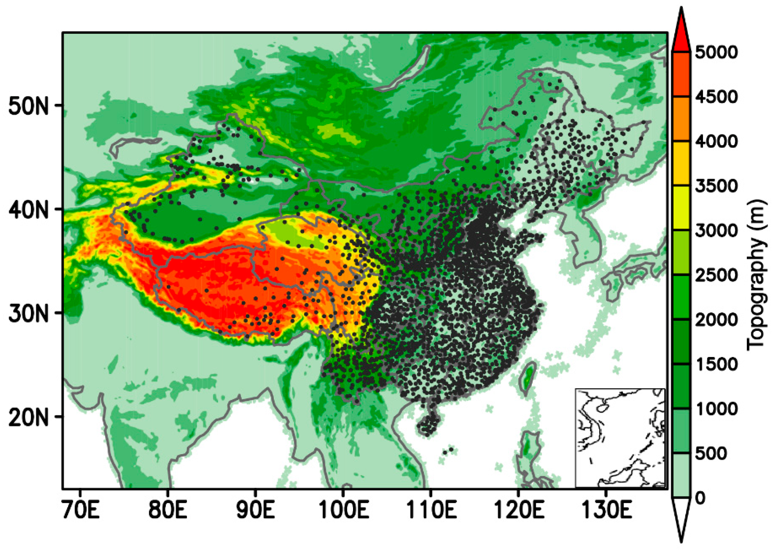
2.2. Data and Verification

The data used in this paper are the ones, provided by the National Meteorological Information Center of China, on the models data of ECMWF, GFS, GRAPES-MESO(Global/Regional Assimilation and Prediction System-Mesoscale Version), and T639 (the products of the Global Medium-range Numerical Prediction System). The spatial resolutions of the outcomes from ECMWF, GFS, GRAPES-MESO, and T639 are 0.125° × 0.125°, 0.5° × 0.5°, 0.1° × 0.1°, and 0.28125° × 0.28125°, respectively. The forecast time is out to 72 h at a 3-hourly temporal resolution. In addition, the observational data (for 2 m temperature) used for verifying the forecasting effect of the model using the VW ensemble method proposed in this paper are the ones from the national surface stations of China provided by the National Meteorological Information Center of China (covering 2380 stations, see Figure 1). Both the model outcomes and observations are used for calculating the VW coefficients (training) and for the comparative analysis of the ensemble forecast effect verification, among which the training period of VW ensemble forecast coefficients is set as September 2015 (the sum of 30 days), and the forecasts verification period as October 2015 (the sum of 31 days) (By the way, it should be mentioned that the model errors would generally not be constant over time. For instance, the model errors in October would usually not be the same as those in September, and thus the selection of the training period of VW ensemble forecast coefficients may be subject to alteration). The index for verification adopts the root-mean-square-errors (RMSEs) between the model forecasts and observations that can be expressed as:
R M S E = 1 n i = 1 n ( X o b s i X mode l i ) 2
where X o b s i stands for the observational value from the stations, and X model i for one from the model outputs, with n being for the total number of observational stations. As a result, a single value is used for each model for verification in this case.
It is needed to interpolate the model forecasts into the 2380 national stations so as to get the errors between forecasts and observations for each station. The interpolating procedure can be simply described as follows: against a certain station, searching four grid points that are nearest to the station, and then making arithmetic average over the values of these four points to get the forecast value. As far as 2 m temperature is concerned, in addition to the procedure above, a height correction is required with the specific procedure as: before interpolating into station from grid points, making first a correction of 2 m temperature forecasts from the model level to the sea level and, then correcting it to the station level after interpolating into the station, based on the standard lapse rate. As for the errors caused by interpolating, the principle of treatment in this paper includes: for the station whose forecasting bias is too large (larger than 100 °C), setting the temperature bias as default (9999.0); in the case of the random error being in line with the normal distribution, rejecting the forecast error mean of an individual model as systematic errors, and, as a result, the weight coefficients are computed after eliminating systematic errors. At the same time, when calculating the estimated value for VW forecasts the systematic errors in the original forecasts are eliminated as well.

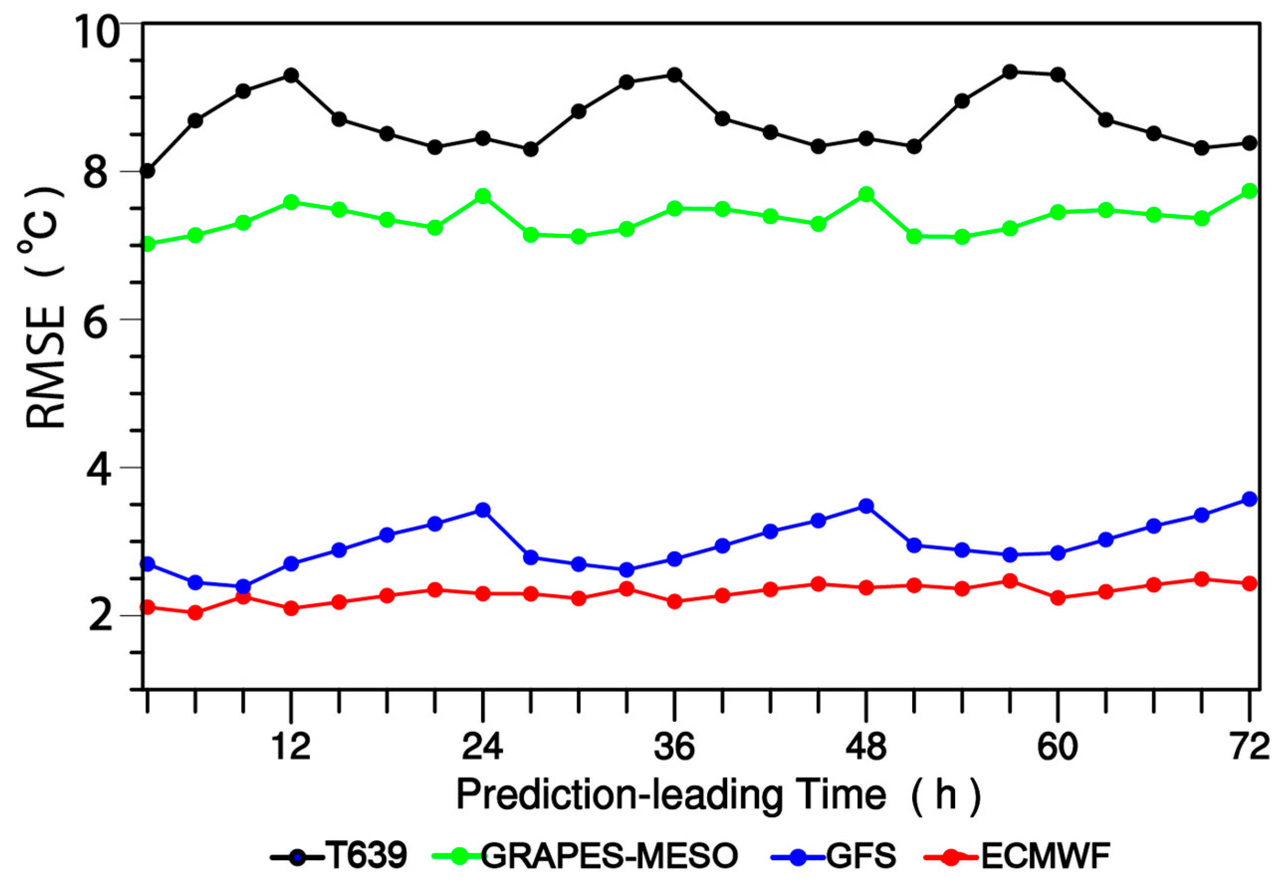
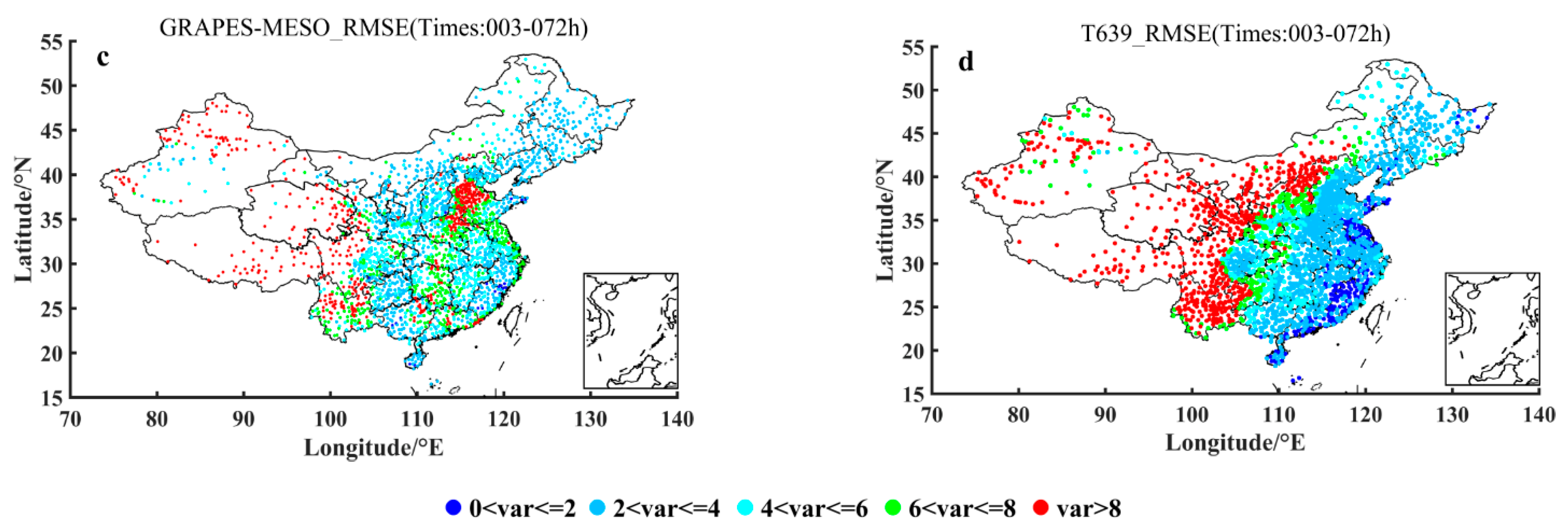
2.3. Performance Analysis of Ensemble Members

In view of that one of the main aims of this paper is to show whether this variant weight method is advantageous, in the case of a worse member added, to suppressing the increase of ensemble forecasts spread or forecast accuracy reduction, it is necessary to first analyze the forecasting effect of the various ensemble members themselves so as to judge their relative quality order, before the predictive results using the VW or EW ensemble method are evaluated. Figure 2 shows the variations of 2 m temperature prediction RMSEs (units: °C) averaged over 2380 surface stations of China in October 2015 with respect to the various prediction leading times for ECMWF, GFS, GRAPES-MESO and T639 models. It is clearly shown in Figure 2 that among them the RMSEs of ECMWF is at minimum in terms of 2 m temperature over China, and moreover, its temporal variation shows a stable performance and its predictive effect is the best. GFS is in the second place, whose predictive errors are larger than those of ECMWF for the leading times of 24, 48 and 72 h with errors closer to those of ECMWF for the other leading times. The predictive errors of GRAPES-MESO and T639 are distinctly larger than those of ECMWF or GFS with GRAPES-MESO forecasts being better than T639 ones. The predictive errors of GRAPES-MESO show a stable performance within 72 h while the maximum errors occur at the leading times of 12, 36 and 57 for T639. As a whole, GRAPES-MESO forecasts are better than T639, GFS better than both GRAPES-MESO and T639, and ECMWF shows the best performance.
Figure 3 shows the spatial distribution of 2 m temperature prediction RMSEs of 2380 surface stations of China in October 2015 with respect to the averaged prediction leading times over the period within 72 h for ECMWF, GFS, GRAPES-MESO and T639 models. The warmer the color of the dot, the larger the RMSEs of the forecast, the lower the accuracy of the forecast, and, at the same time, the deeper the cold tone, the smaller the RMSEs of the forecast and the higher the accuracy of the forecast. It can be seen from Figure 3 that the prediction errors of ECMWF in the national stations range is almost all between 0 and 4 °C, and in particular, the prediction accuracy is higher in southeastern China. The prediction accuracy of GFS in the second place is weakened in both the south and north of Qinling Mountains, with the southeast coastal area maintaining the same effect as ECMWF. GRAPES-MESO has a tendency to increase RMSEs in northwestern China and the Beijing-Tianjin-Hebei region, with the RMSEs greater generally than 4 °C; T639 forecasts are more complicated, that is, in most of the west of Taihang Mountains the RMSEs are greater than 8 °C, and the east of the Taihang Mountains are dominated by RMSEs of 2–4 °C.
According to the analyses above, next we will adopt the two models of ECMWF and GFS that show the best performance as the 2-models ensemble members, and for the 3-models ensemble forecasts the ensemble members consist of these two members above plus GRAPES-MESO, and finally for the 4-models ensemble forecasts the members cover one more model of T639 on the basis of the 3-models ensemble members (See Table 1). The multi-model combined design is mainly aimed at comparing and analyzing the effect of the continuous addition of the members of poorer models on the ensemble forecasting results between the VW and the EW method.

3. A Brief Introduction to the Principle of the VW Method and Its Superiority

There exists a great difference among the outputs from the various ensemble forecast models, which might be attributable either to the problems caused by the data assimilation program generating the initial values of each ensemble member, or to the imperfection of the physical process parameterization itself that is incorporated into the ensemble, even to the inherent difficulty of the computational geophysical fluid dynamics and so on. However, it has been being a serious challenge how to judge which is better or worse with regard of the various ensemble systems. As far as the physical connotation and preliminary applications of the computational method for the weight coefficient of various ensemble members through reciprocal of variance error, as proposed by Sun et al. [43], is concerned, it seems that there should be good prospects for development. By the so-called reciprocal of variance error, it is meant that the weight coefficient of each of the ensemble members is inversely proportional to their respective variance error. Therefore, on the basis of the proof by Sun et al. [43] as to the rationality or its scientific foundation, it is urgent to more rigorously prove why the variant weight (VW) coefficient computational method through reciprocal of variance error is better than the equal weight (EW) method for various ensemble forecast cases and thus the forecast accuracy is able to be improved.
As seen in Appendix A at the end of this paper, through calculation of a best estimate of the mean forecasts by the VW method, the variant weight ensemble mean (VWEM) at the time step of t + 1, that is named as X ^ (x, y, z, t + 1) in this paper, can be worked out (Appendix A.1). Thus, we are able to distinguish with the conventional ‘equal weight ensemble mean (EWEM)’. Obviously, VWEM is closely related to the weight for ensemble members, while EWEM not.
On the other hand, it is easily found that, via comparative analysis of accuracy between VW and EW ensemble forecasts, VW ensemble forecasts are better than EW ensemble forecasts. Or alternatively, the VW method performs better than the EW method because of the forecast error variance using the VW method being smaller than that using the EW method (Appendix A.2).
In addition, based on the comparative analyses of influence of adding ensemble model member on VW and EW forecast accuracy, an interesting outcome has been revealed. Specifically, a single model (even one with a lower forecast accuracy) incorporated into the ensemble is able to enhance the forecast accuracy (at least not lower the accuracy). Moreover, it is distinctly seen that the ensemble forecast accuracy is superior to that of any of the models (say, ECMWF) participated in the ensemble due to the sum of the weights of the multiple models be larger than the weight of any single model therein (Appendix A.3).

4. Example Verification

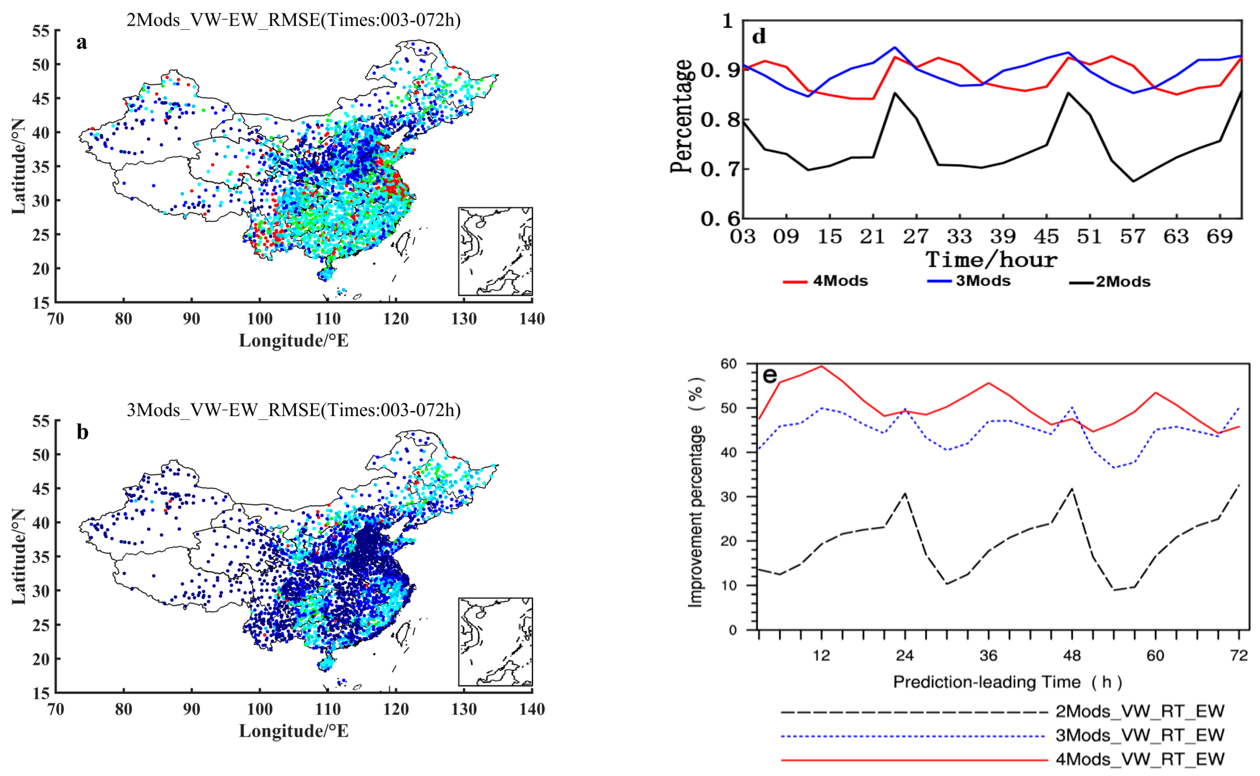
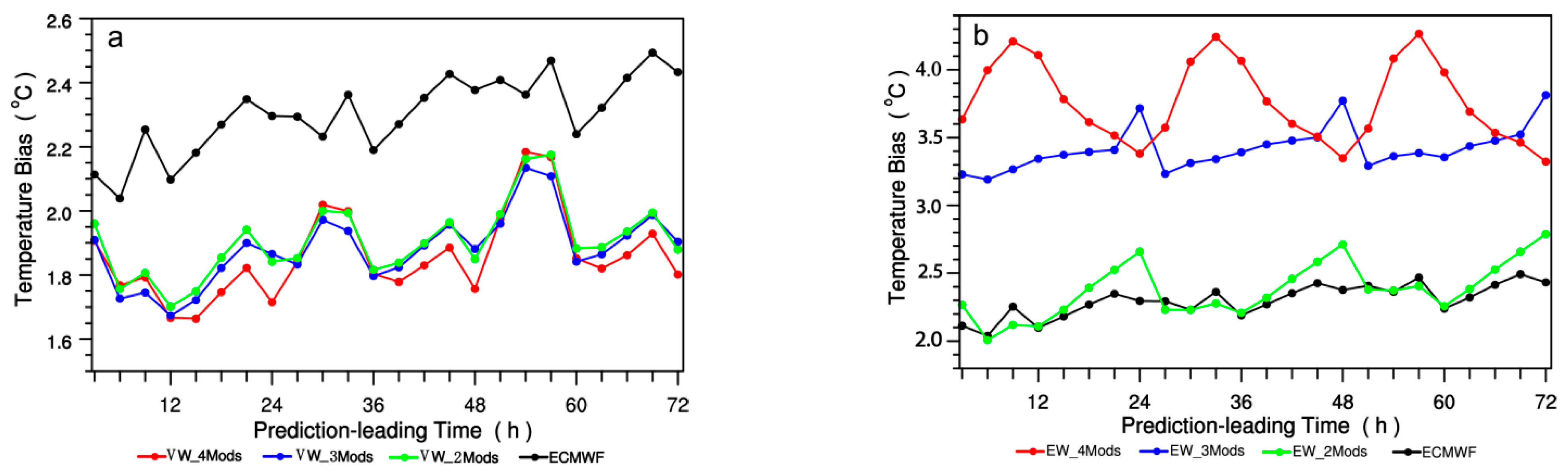
4.1. Comparative Analysis of Ensemble Forecasts between VW and EW Methods

In the theoretical derivation in Section 3 as well as in Appendix A, we have proved that the ensemble prediction using the VW method is better than the ensemble prediction using the EW method. This section will verify the theoretical results by comparing and analyzing the effects of ensemble prediction of VW and EW methods under different combinations of models based on the real observations. Figure 4 shows the averaged variations of 2 m temperature prediction RMSEs over 2380 surface stations of China for October 2015 with respect to the various prediction leading times for the 2-, 3- and 4-models ensemble forecasting using VW and EW ensemble methods as compared with that of the ECWMF forecasting. The averaged 2 m temperature prediction RMSEs of ECMWF over 2380 surface stations of China for October 2015 with respect to the various prediction leading times are between 2.0–2.6 °C while ones of the 2-, 3- and 4-models ensemble forecasting using the VW method are all between 0.1–0.2 °C. It is seen from Figure 4 that for either 2-, 3-, or 4-models ensemble forecasts, the forecasting effect of using the VW method is obviously better than that of the EW method, and with the increase of the number of model members, the forecasting advantage of using the VW method is more obvious. On the other hand, according to the distributions of the 2 m temperature prediction RMSEs difference between VW and EW ensemble methods for 2-, 3- and 4-models ensemble forecasting (Figure 5), it is found that, for most stations of China (more than 70%; Figure 5d), the ensemble prediction effect using the VW method is better than the ensemble prediction effect using the EW method (the difference is less than zero), with either 2- (Figure 5a), 3- (Figure 5b), or 4-models (Figure 5c) ensemble forecasts taken into consideration. As far as the improvement percentage of the ensemble forecasting (Figure 5e) is concerned, the VW method of different multi-model combinations has a significant improvement in the 2 m temperature forecasts against the EW method (both positive percentages). At the same time, with the increase of model members (2 models to 4 models ensemble prediction), the 2 m temperature prediction effect of the VW method is more improved than the EW method with the fractional percentage improvement (Sun et al., 2017) enhanced from 20% to nearly 55%. Therefore, as shown by the averaged 2 m temperature forecasts over 2380 surface stations of China, VW methods have obvious advantages over EW methods in terms of either the absolute errors value or the relative errors value.

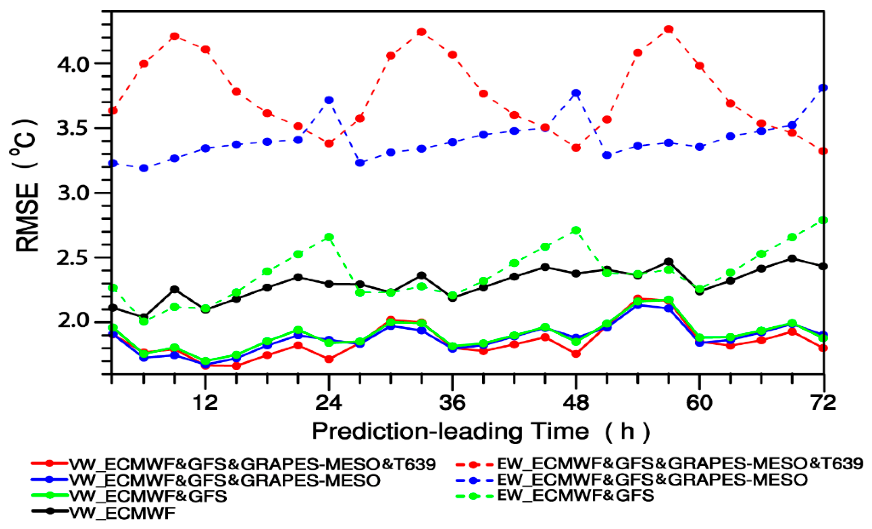
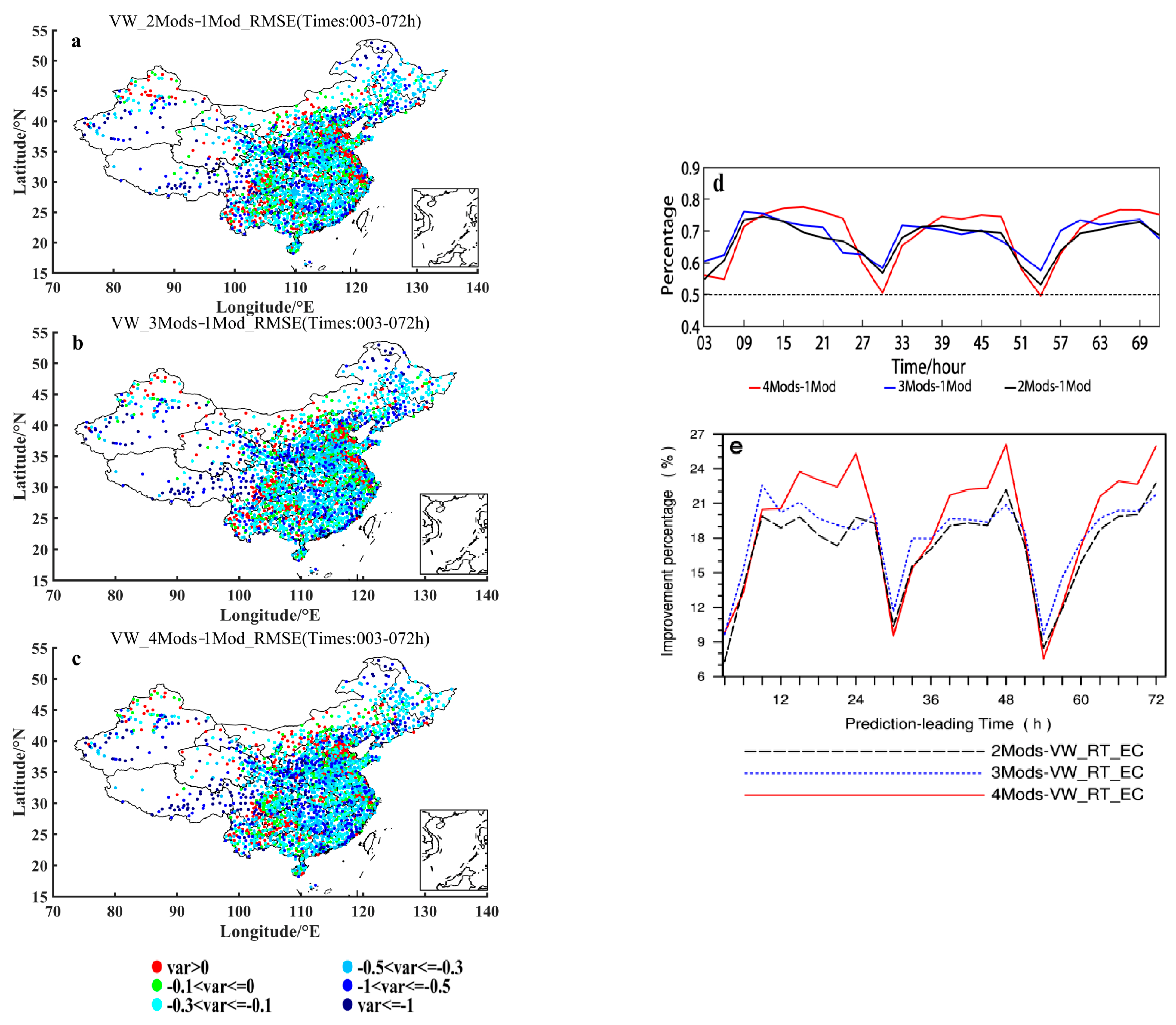
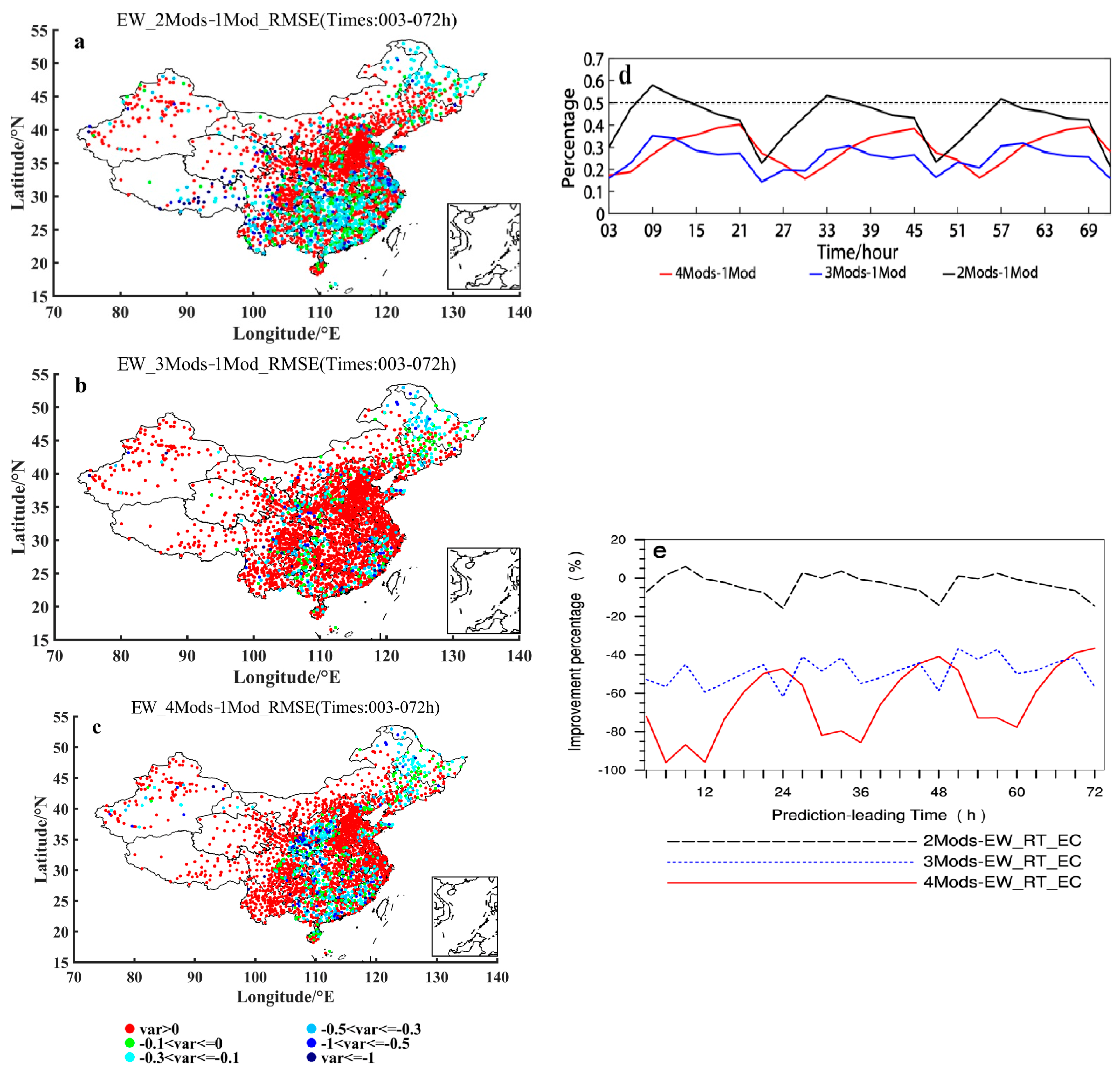
4.2. The Superiority of VW over EW Methods as Shown by the Combination Prediction Verification

We have theoretically proved that when the model with poorer forecasting effect is added to the model with better forecasting effect, the results obtained by using the VW method and the EW method are completely opposite. The multi-model combination design is mainly for the purpose of comparative analysis of the influence of continuously adding poorer model members on the ensemble prediction effect between VW and EW methods. Figure 6a,b show the comparison of RMSEs to that of the ECMWF forecasting for the 2-, 3- and 4- models ensemble forecasting using (a) VW and (b) EW ensemble methods, respectively. Figure 6a shows that there exists such a relation in terms of the RMSEs size of VW forecasting among these four model combinations: 4-models < 3-models < 2-models < a single model (ECMWF). Specifically, RMSEs of 4-models is at minimum with the highest forecasting accuracy, RMSEs of 3-models at the leading times of 12–27 h, 36–51 h, and 60–72 h are all larger than ones of 4-models, RMSEs of 2-models are all larger than ones of 3-models except at the leading times of 24 h, 48 h and 72 h, and the single model of ECMWF has the maximum RMSEs. With the gradual addition of the poorer model members, the forecasting accuracy of the VW method is gradually improved and stabilized for 70.83% of the leading times, which indicates that a better model added by a poorer model member using the VW method can suppress the phenomenon of the ensemble forecast spread increasing (or the forecast accuracy gradual decreasing). On the other hand, if the EW method is employed, the RMSEs size relation becomes opposed: 4-models > 3-models > 2-models > a single model (ECMWF). All of these four sets of ensemble combination have maximum at 24 h, 48 h and 72 h in terms of RMSEs. With the gradual increase of the members of the poorer model, the forecasting effect of the EW method is getting more and more unstable, with the forecast RMSEs increased gradually, and the overall deviation being above 2 °C.
Figure 7a–c show the distributions of the 2 m temperature ensemble forecasting RMSEs differences between 2-models and ECMWF-model, 3-models and ECMWF-model, and 4-models and ECMWF-model, respectively, using the VW ensemble method. It can be seen from these panels of (a)–(c) in Figure 7 that in the case of gradual increasing the members with poorer forecasting accuracy, most of the stations satisfy still the condition of being smaller than zero when the VW method is used. That is, in the case of the VW method employing, for most of the stations of China the RMSEs of multi-model forecasts are smaller than ECMWF model even in the case of gradual increasing the members with poorer forecasting accuracy. Figure 7d shows also that the number of stations with the difference of multi-model forecasts RMSEs minus ECMWF’s RMSEs being smaller than zero reaches basically the ratio being larger than 60%, for the case of either 2-models, 3-models or 4-models minus 1-model that is ECMWF model, with a little bit smaller 60% (but still larger than 50%) at the leading times of 24 h, 48 h and 72 h. As a matter of fact, owing to 1 Model being just ECMWF as shown in Table 1, Figure 7d results in nature from Figure 4. Based on Figure 4 the calculated negative 2 m temperature prediction RMSEs differences between 2 and 1 (2Mods-1Mod), 3 and 1 (3Mods-1Mod), and 4 and 1 (4Mods-1Mod) models ensemble forecasting using the VW ensemble method would distinctly show a decrease around 30 h and 54 h, which is directly caused by the fact that the distance between the curve for ECMWF forecasting and the curve for the 2-, 3- or 4-models ensemble forecasting using the VW ensemble method is extremely short around 30 h and 54 h. As far as the relative improvement percentage of the 2-, 3- and 4-models ensemble forecasting to ECMWF is concerned (Figure 7e), all the multi-model ensemble forecasts show an improvement to some extent (positive percentage). Even in the case of gradual increasing (from 2- to 4-models) model members with poorer performance, the relative improving amplitude does not drop but rise. It is thus evident that for the ensemble forecasting using the VW method, the effect is stable and it keeps the 2 m temperature forecasting effect of the half and above stations better than the ECMWF one despite of increasing continuously the model members with poorer performance.
Figure 8a–c show the distributions of the 2 m temperature ensemble forecasting RMSEs differences between 2-models and ECMWF-model, 3-models and ECMWF-model, and 4-models and ECMWF-model, respectively, using the EW ensemble method. It can be seen from these panels of (a)–(c) in Figure 8 that most stations of China have values greater than zero. That is, in the case of the EW method used, the RMSEs of the multi-model ensemble forecasts are significantly larger than the RMSEs of the ECMWF forecasts. It can also be seen from Figure 8d that in the case of increasing the number of poorer model members, the situation that the RMSEs of the multi-model ensemble forecasts using the EW method is smaller than the RMSEs of the ECMWF forecasts occurred in less than half of the stations of China. The proportion of the stations with better results is only below 40% on average within 72 h of forecast leading time (among them 25% for 3- and 4-models ensemble forecasts, and 40% for 2-models). And with the increase of the members of the poorer model, the ratio of the number of stations with multi-model ensemble forecasts better than the ECMWF forecasts is obviously decreasing, specifically decreasing from 40% for 3- and 4-models to 25% for 2-models (on average within 72 h of forecast leading time). In terms of the improvement rate of the multi-model ensemble forecasting using the EW method relative to the ECMWF forecasting (Figure 8e), the multi-model forecasts using the EW method become worse than the ECMWF forecasts (basically as negative improvement rate), and with the increase of the members of the poorer model, the multi-model ensemble forecasts become even worse compared with the ECMWF predictive effect. That is to say, in the case of increasing the number of poorer model members, the predictive results of most of the national stations using the EW method and their average ensemble predictive effect will be worse than the ECMWF, and become worse with the increase of the poorer members.

5. Conclusions and Discussion

The method of calculating the respective weights by reciprocal of the variance of the ensemble members is one of the effective methods for the development of ensemble forecast products. Previous studies have mainly applied this method to the ensemble prediction of precipitation, but due to the discontinuity of precipitation, it is often difficult to obtain a reasonable weight distribution. Sun et al. (2017) applied this method to ensemble prediction of continuous temperature, showing good prediction results. However, they did not use the observed temperature data as the true values for calculating the variance and corresponding weight of the ensemble members, and at the same time, the theoretical derivation of the predictive variance comparison of the VW vs. EW method has not yet been given. On the other hand, it is worthwhile to discuss whether the VW method is beneficial to suppressing the increase of the ensemble forecast spread or the decrease of the forecast accuracy in the case of increasing the poorer ensemble members, which has not been investigated by previous studies either. Therefore, this paper firstly proves theoretically that the VW method is superior to the ensemble forecasting of the EW method, and then reveals the advantage of the ensemble forecasting using the VW method in the case of increasing the ensemble membership of the poorer model. On this basis, the 2 m temperature observations of 2380 national basic stations of China in September 2015 and the multiple models (ECMWF, GFS, GRAPES-MESEO and T639) were used to train and get the VW coefficients for the various models. Then, based on the comparative analyses of the 2 m temperature observations of these stations in October 2015 with the multi-model ensemble prediction values obtained using the VW coefficients (taking the RMSEs as the evaluation index) the theoretical derivation results are verified. The main analyses and results are as follows:
(1) The VW ensemble forecasting is significantly better than the single deterministic forecasting. In terms of the multi-model (2-, 3- or 4-models) 2 m temperature prediction, the ensemble predictive effect using the VW method proposed in this paper is distinctly better than that of the best single model deterministic forecasts (ECMWF forecasts) participating in the ensemble. In contrast, the multi-model ensemble predictive effect using the EW method is worse than the single-model deterministic forecast.
(2) The averaged 2 m temperature prediction RMSEs of ECMWF over 2380 surface stations of China for October 2015 with respect to the various prediction leading times are between 2.0–2.6 °C while ones of the 2-, 3- and 4-models ensemble forecasting using the VW method are all between 0.1–0.2 °C. The ensemble predictive effect of the VW method is obviously better than the EW method. From the view of individual stations, for more stations of China than 70%, the ensemble prediction effect using the VW method is better than the ensemble prediction effect using the EW method, with either 2-, 3-, or 4-models ensemble forecasts taken into consideration. For the ensemble forecasts of 2 m temperature by the different model ensemble member combinations (2-, 3- and 4-models), the national stations-averaged ensemble prediction effect using the VW method proposed in this paper is distinctly better than that using the EW method. With the increase of model members (2 models to 4 models ensemble prediction), the 2 m temperature prediction effect of the VW method is more improved than the EW method (relative improvement rate is enhanced from 20% to nearly 55%).
(3) The VW method is advantageous for solving the problem of reduced accuracy of ensemble prediction due to the addition of poorer model members. In the case of increasing the number of poorer model members, in terms of the national stations average and for 60% of the national individual stations, the RMSEs of the 2 m temperature ensemble forecasts using the VW method of this paper are smaller than the ECMWF forecasts, and with the increase of the poorer ensemble members, the accuracy of the ensemble prediction remains stable. On the contrary, in the case of increasing the poorer model members, in terms of the national stations average and for 60–75% of the individual stations nationwide, the RMSEs of the 2 m temperature ensemble forecasts using the EW method are larger than the ECMWF forecasts, and with the increase of poorer ensemble member, the accuracy of ensemble prediction is significantly reduced.
The above results show that the VW method performs better than the EW method in the case of either general multi-model combination or increasing the poorer model members. Indeed, it is distinctly potential that there exist some exemptions in the case-computational results since the theoretical proof done in this paper is made under the assumption. On the other hand, how to update the VW method proposed in this paper so as to make the forecasting effect increase more obviously when the model member number increases is a question worthy of further discussion. This problem may be related to the variant weights of this paper that are obtained by the prior variance calculation. In the near future, we are going to design a number of schemes of weights construction for the forecasting training phase, which include the way of calculating the model weights through obtaining the 3-hourly model errors over a longer period of model forecasts in, say, for our present case, October and apply it to October 2015. In addition, calculating the weight via posterior variance may be an effective way to solve the problem. On the other hand, how to optimize weights for different regions and different time periods is also a problem that needs further study. For example, from the dot diagram in Figure 7 and Figure 8, it can be seen that the advantage of using the VW method in the station forecasting in the southeastern region of China is more obvious, but it does not cover all the stations in the whole country. Therefore, how to enhance the universality of the VW method is the next work to be done as well.

Author Contributions

Conceptualization, X.W., X.S., J.Y. and J.S. (Jing Sun); methodology, X.W., X.S., J.S. (Jilin Sun) and J.Y.; software, X.W., J.S. (Jing Sun) and C.L.; validation, X.W., J.S. (Jing Sun) and C.L.; formal analysis, X.W., J.S. (Jing Sun) and J.Y.; investigation, X.W., X.S., J.S. (Jilin Sun) and J.Y.; resources, X.W., X.S. and J.S. (Jing Sun); data curation, X.W., X.S. and J.Y.; writing—original draft preparation, X.W. and J.S. (Jing Sun); writing—review and editing, X.W., X.S., C.L.; visualization, X.W. and J.S. (Jilin Sun); supervision, X.W. and X.S.; project administration, X.W., X.S. and J.S. (Jilin Sun); funding acquisition, X.S. All authors have read and agreed to the published version of the manuscript.

Funding

This research was funded by the National key research and development program of China (2018YFC1506606) and Key project of basic scientific research operating expenses of Chinese Academy of Meteorological Sciences(2019Z003).

Institutional Review Board Statement

Not applicable.

Informed Consent Statement

Not applicable.

Data Availability Statement

The models and surface observation data used in the research are available from the datasets of the National Meteorological Information Center of China. They are not publicly available.

Acknowledgments

Not applicable.

Conflicts of Interest

The authors declare no conflict of interest.

Appendix A

Theoretical proof of improving forecast accuracy using the variant weight multi-model ensemble method.

Appendix A.1. Calculation of a Best Estimate of the Mean Forecasts by the VW Ensemble Method

Supposing there are m models and assuming they are uncorrelated to each other, the weight matrix P is first calculated according to the historical forecast error:
P = σ 0 2 D 1 = P 1 0 0 0 P 2 0 0 0 P m ,
Here, σ 0 2 is a unit “weight variance”, which can be any value and in this study σ 0 2 = 1 is chosen; the elements in the weight matrix are the covariance-based quantity with P1, P2 …, Pm standing for the weights of the m models in proper sequence and the others as zero since it is independent from each other; D is the covariance matrix of the forecast error for the models in terms of variance and can be expressed as:
D = σ ^ 1 2 0 0 0 σ ^ 2 2 0 0 0 σ ^ m 2 ,
On the other hand, the error equations for the ensemble forecast model members can be written as:
V m * 1 = A m * 1 X ^ m * 1     L m * 1 ,
where L m * 1 is the forecast value from each model, V m * 1 is the correction of L m * 1 , A m * 1 is an m-dimensional sequence vector whose value is all 1, and X ^ is just the best estimate of the ensemble mean forecasts; in terms of matrix, L m * 1 ,  V m * 1 and A m * 1 can be written respectively as:
L m * 1 = L 1 L 2 L m T , V m * 1 = V 1 V 2 V m T , A m * 1 = 1 1 1 T .
According to the principle of the least square method, under the condition of V T P V = min , the optimal valuation of the ensemble mean forecasts X ^ can be worked out as:
X ^ = A T P A 1 A T P L = i = 1 m P i ( x , y , z ) L i ( x , y , z , t + 1 ) i = 1 m P i ( x , y , z )
This best estimate X ^ at the time of t + 1 from the forecast L i ( t + 1 ) is named in this paper as ‘variant weight ensemble mean (VWEM)’, so as to distinguish with the conventional ‘equal weight ensemble mean (EWEM)’ (Cane and Milelli, 2006).

Appendix A.2. Comparative Analysis of Accuracy between VW and EW Ensemble Forecasts

The forecast accuracy analysis is usually made via comparing the forecasts variance between various models. The total error variance of m models σ t o t a l 2 is set as
σ t o t a l 2 = i = 1 m σ ^ L i 2 = m σ ¯ L 2
where σ ¯ L 2 is the averaged forecast error variance over the m models, and σ ^ L i 2 is the forecast error variance for the ith model. By the definition for the weight coefficient P i , σ ^ L i 2 = σ 0 2 P i where σ 0 2 is a “unit weight variance” with σ 0 2 = 1 chosen in this paper (Cane and Milelli, 2006), and thus, according to the variance-covariance propagation law, the VW ensemble forecast variance σ X ^ 2 can be written as σ X ^ 2 = σ 0 2 i = 1 m P i . Furthermore, for comparison purposes with that of the EW ensemble, it can be re-written as σ ¯ L 2 i = 1 m σ ¯ L 2 σ ^ L i 2 while the EW ensemble forecast variance can be written as σ ¯ L 2 m since in this case σ X ^ 2 = i = 1 m σ ^ L i 2 m 2 based on the variance-covariance propagation law. As a result, if we could have proved that
i = 1 m σ ¯ L 2 σ ^ L i 2 m
it then means that VW ensemble forecasts are better than the EW ensemble forecasts.
For the sake of simplicity, setting
σ ¯ L 2 = a ,   σ ^ L i 2 = b i ,
Equation (A7) then becomes
i = 1 m a b i m
Since σ ¯ L 2 is the averaged variance over the m models, setting
a = 1 m i = 1 m b i
and substituting it into Equation (A8) may lead to
i = 1 m 1 + j i m b j b i m 2
Equation (A11) can be rewritten as
i = 1 , j = 1 m b i b j + b j b i i j m ( m 1 )
On the other hand, owing to ( b i b j ) 2 0 , that is, b i 2 + b j 2 2 b i b j , we have
b i b j + b j b i = b i 2 + b j 2 b i b j 2
Accordingly, it can be gotten that
i = 1 , j = 1 m b i b j + b j b i i j 2 C m 2 = 2 m ( m 1 ) / 2 = m ( m 1 )
where C m 2 is the combination symbol, standing for the number of categories of any two different numbers selecting from m numbers. In our case, i = 1 , j = 1 m b i b j + b j b i i j means that there is the sum of m ( m 1 ) / 2 terms with the form like b i b j + b j b i so that we have the Equation (A14) reached.
It is seen that the Equation (A14) is in keeping with (A12). This suggests that the Equation (A12) or (A7) comes into existence, that is, VW ensemble forecasts are better than EW ensemble forecasts. Or alternatively, the VW method performs better than the EW method because of the forecast error variance using the VW method being smaller than one using the EW method.

Appendix A.3. Influence of Increasing Ensemble Model Member on VW and EW Forecast Accuracy

Here we recall that under the condition that the models are non-related to each other, the best estimate and variance of VWEM and EWEM are respectively:
(For VWEM)
X ^ = i = 1 m P L i L i i = 1 m P L i ,   and σ X ^ 2 = σ 0 2 i = 1 m P i ,   and
(For EWEM)
X ^ = i = 1 m L i m   , and   σ X ^ 2 = i = 1 m σ ^ L i 2 m 2
Next one will discuss the influence of incraesing ensemble model member on VW and EW forecast accuracy.
For VWEM, if a single model (even if one with a lower forecast accuracy) is incorporated into the ensemble, that is, the number of models is increased from m to m + 1, the variance of the ensemble forecasts becomes:
σ X ^ ( m + 1 ) 2 = σ 0 2 i = 1 m P i + P m + 1
According to the definition of the weight P (see Equation (1)), P is non-negative, and thus we have
i = 1 m P i + P m + 1 i = 1 m P i
and further
σ X ^ ( m + 1 ) 2 σ X ^ m 2
which suggests that, a single model (even one with a lower forecast accuracy) incorporated into the ensemble is able to enhance the forecast accuracy (at least not lower the accuracy). In addition, it is easily seen that the ensemble forecast accuracy is superior to that of any model (say, ECMWF) participated in the ensemble due to the sum of the weights of the multiple models be larger than the weight of any single model therein.
On the other hand, for EWEM, the variance of the ensemble forecasts for m + 1 models based on Equation (A16) is
σ 2 X ^ ( m + 1 ) = i = 1 m σ i 2 + σ i + 1 2 ( m + 1 ) 2
To ensure the accuracy of the equal-weight ensemble mean with the model member number of m + 1 being higher than that of the ensemble with the member number of m it is needed that
σ X ^ ( m + 1 ) 2 σ X ^ m 2
According to Equation (A16) and Equation (A20), Equation (A21) can be rewritten as
σ i + 1 2 2 m + 1 m σ ¯ 2
where σ ¯ 2 = 1 m i = 1 m σ i 2 .
Therefore, only under the condition that Equation (A22) is met, it might be ensured that the accuracy of the equal-weight ensemble mean with the model member number of m + 1 is higher than that of the ensemble mean with the member number of m. This implies that a model with poorer performance incorporated into the ensemble would potentially reduce accuracy of the equal-weight ensemble mean.

References

  1. Tracton, M.S.; Kalnay, E. Operational ensemble prediction at the national meteorological center: Practical aspects. Weather Forecast. 1993, 8, 379–398. [Google Scholar] [CrossRef]
  2. Molteni, F.; Buizza, R.; Palmer, T.N.; Petroliagis, T. The ECMWF ensemble prediction system: Methodology and validation. Q. J. R. Meteor. Soc. 1996, 122, 73–119. [Google Scholar] [CrossRef]
  3. Velazquez, A.J.; Petit, T.; Lavoie, A.; Boucher, M.-A.; Turcotte, R.; Fortin, V.; Anctil, F. An evaluation of the Canadian global meteorological ensemble prediction system for short-term hydrological forecasting. Hydrol. Earth Syst. Sci. 2009, 13, 2221–2231. [Google Scholar] [CrossRef] [Green Version]
  4. Descamps, L.; Labadie, C.; Joly, A.; Bazile, E.; Arbogast, P.; Cébron, P. PEARP, the Météo-France short-range ensemble prediction system. Q. J. R. Meteor. Soc. 2014, 141, 1671–1685. [Google Scholar] [CrossRef]
  5. Bowler, E.N.; Arribas, A.; Mylne, K.R.; Robertson, K.B.; Beare, S.E. The MOGREPS short-range ensemble prediction system. Q. J. R. Meteorol. Soc. 2008, 134, 703–722. [Google Scholar] [CrossRef]
  6. Garcia-Moya, A.J.; Callado, A.; Santo, C.; Santos-Muñoz, D.; Simarro, J. Predictability of Short-Range Forecasting: A Multimodel Approach. Nota Técnica 1 del Servicio de Predecibilidady Predicciones Extendidas (NT SPPE-1); Agencia Estatal de Meteorologia (AEMET), Ministerio de Medio Ambiente, y MedioRural y Marino: Madrid, Spain, 2009. [Google Scholar]
  7. Frogner, L.I.; Haakenstad, H.; Iversen, T. Limited-area ensemble predictions at the Norwegian Institute. Q. J. R. Meteorol. Soc. 2006, 132, 2785–2808. [Google Scholar] [CrossRef]
  8. Marsigli, C.; Montani, A.; Pacagnella, T. A spatial verification method applied to the evaluation of high-resolution ensemble forecasts. Meteorol. Appl. 2008, 15, 125–143. [Google Scholar] [CrossRef]
  9. Yamaguchi, M.; Sakai, R.; Kyoda, M.; Komori, T.; Kadowaki, T. Typhoon ensemble prediction system developed at the Janpan Meteorological Agency. Mon. Weather Rev. 2009, 137, 2592–2604. [Google Scholar] [CrossRef]
  10. Park, S.; Kim, D.; Lee, S.; Lee, K.; Kim, J.; Song, E.; Seo, K. Comparison of extended medium-range forecast skill between KMA ensemble, ocean coupled ensemble, and GloSea5. Asia-Pac. J. Atmos. Sci. 2017, 53, 393–401. [Google Scholar] [CrossRef]
  11. Ebert, E.E. Ability of a poor man’s ensemble to predict the probability and distribution of precipitation. Mon. Weather Rev. 2001, 129, 2461–2480. [Google Scholar] [CrossRef]
  12. Otsuka, S.T.; Miyoshi, A. Bayesian optimization approach to multimodel ensemble Kalman filter with a low-order model. Mon. Weather Rev. 2015, 143, 2001–2012. [Google Scholar] [CrossRef]
  13. Buizza, R.; Palmer, T.N. Impact of ensemble size on ensemble prediction. Mon. Weather Rev. 1988, 126, 2503–2518. [Google Scholar] [CrossRef]
  14. Jonson, A.; Wang, X.G.; Xue, M.; Kong, F.; Zhao, G.; Wang, Y.; Thomas, K.W.; Brewster, K.A.; Gao, J. Multiscale characteristics and evolution of perturbations for warm season convection-allowing precipitation forecast: Dependence on background flow and method of perturbation. Mon. Weather Rev. 2014, 142, 1053–1073. [Google Scholar] [CrossRef]
  15. Wang, Y.M.; Bellus, J.F.; Geleyn, X.; Ma, H.; Tian, H.; Weidle, F. A new method for generating initial condition perturbations in a regional ensemble prediction system: Blending. Mon. Weather Rev. 2014, 142, 2043–2059. [Google Scholar] [CrossRef] [Green Version]
  16. Sonia, J.; Juan, P.M.; Pedro, J.G.; Juan, G.N.J.; Raquel, L.P. A multi-physics ensemble of present-day climate regional simulations over the Iberian Peninsula. Clim. Dyn. 2013, 40, 3023–3046. [Google Scholar]
  17. Lee, A.J.; Haupt, S.E.; Young, G.S. Down-selecting numerical weather prediction multi-physics ensembles with hierarchical cluster analysis. J. Climatol. Weather. Forecast. 2016, 4, 156. [Google Scholar]
  18. Garcia-Ortega, E.; Lorenzana, J.; Merino, A.; Fernandez-Gonzalez, S.; Lopez, L.; Sanchez, J.L. Performance of multi-physics ensembles in convective precipitation events over northeastern. Spain Atmos. Res. 2017, 190, 55–67. [Google Scholar] [CrossRef]
  19. Zhang, Z.; Krishnamurti, T.N. Ensemble forecasting of hurricane tracks. Bull. Amer. Meteor. Soc. 1997, 78, 2785–2795. [Google Scholar] [CrossRef] [Green Version]
  20. Du, J.; Mullen, S.L.; Sanders, F. Short-range ensemble forecasting of quantitative precipitation. Mon. Weather Rev. 1997, 125, 2427–2459. [Google Scholar] [CrossRef]
  21. Zhi, F.X.; Qi, H.X.; Bai, Y.Q.; Lin, C. A comparison of three kinds of multimodel ensemble forecast techniques based on the TIGGE data. Acta Meteor. Sin. 2012, 26, 41–51. [Google Scholar] [CrossRef]
  22. Zhi, F.X.; Zhang, L.; Bai, Y.Q. Application of the Multimodel Ensemble Forecast in the QPF. In Proceedings of the International Conference on Information Science and Technology, Nanjing, China, 26–28 March 2011; pp. 657–660. [Google Scholar] [CrossRef]
  23. Zhi, X.F.; Bai, Y.Q.; Lin, C. Multimodel super ensemble forecasts of the surface air temperature in the Northern Hemisphere. In Proceedings of the Third THORPEX International Science Symposium, Monterey, CA, USA, 14–18 September 2009; WMO: 57. Available online: https://www.researchgate.net/publication/303486757_Superensemble_forecasts_of_the_surface_temperature_in_Northern_Hemisphere_middle_latitudes (accessed on 24 January 2022).
  24. Krishnamurti, N.T.; Sagadevan, A.D.; Chakraborty, A.; Mishra, A.K.; Simon, A. Improving multimodel weather forecast of monsoon rain over China using FSU superensemble. Adv. Atmos. Sci. 2009, 26, 813–839. [Google Scholar] [CrossRef]
  25. Zheng, M.; Chang, K.E.; Colle, A.B. Evaluating US East Coast winter storms in a multimodel ensemble using EOF and clustering approaches. Mon. Weather Rev. 2019, 147, 1967–1987. [Google Scholar] [CrossRef]
  26. Evans, E.R.; Harrison, M.S.J.; Graham, R.J.; Mylne, K.R. 2000: Joint medium-range ensembles from the Met. Office and ECMWF systems. Mon. Weather Rev. 2000, 128, 3104–3127. [Google Scholar] [CrossRef]
  27. Du, J. Uncertainty and Ensemble Forecasting. NOAA/NWS Science and Technology Infusion Lecture Series. 2007. Available online: http://www.nws.noaa.gov/ost/climate/STIP/uncertainty.htm (accessed on 24 January 2022).
  28. Qi, L.; Yu, H.; Chen, P. Selective ensemble-mean technique for tropical cyclone track forecast by using ensemble prediction systems. Q. J. R. Meteor. Soc. 2014, 140, 805–813. [Google Scholar] [CrossRef]
  29. Raftery, A.E.; Gneiting, T.; Balabdaoui, F.; Polakowski, M. Using Bayesian model averaging to calibrate forecast ensembles. Mon. Weather Rev. 2005, 133, 1155–1174. [Google Scholar] [CrossRef] [Green Version]
  30. Liu, J.G.; Xie, Z.H. BMA probabilistic quantitative precipitation forecasting over the Huaihe basin using TIGGE multimodel ensemble forecasts. Mon. Weather Rev. 2014, 142, 1542–1555. [Google Scholar] [CrossRef] [Green Version]
  31. Bouallegue, Z.B. Calibrated short-range ensemble precipitation forecasts using extended logistic regression with interaction terms. Wea. Forecast. 2013, 28, 515–524. [Google Scholar] [CrossRef]
  32. Weigel, P.A.; Liniger, M.A.; Appenzeller, C. Can multi-model combination really enhance the prediction skill of probabilistic ensemble forecasts? Q. J. R. Meteor. Soc. 2008, 134, 241–260. [Google Scholar] [CrossRef]
  33. Yun, W.T.; Stefanova, L.; Mitra, A.K.; Vijaya Kumar, T.S.V.; Dewar, W.; Krishnamurti, T.N. A multi-model superensemble algorithm for seasonal climate prediction using DEMETER forecasts. Tellus A Dyn. Meteorol. Oceanogr. 2005, 57, 280–289. [Google Scholar] [CrossRef]
  34. Cane, D.; Milelli, M. Weather forecasts obtained with a Multimodel SuperEnsemble Technique in a complex orography region. Meteorol. Z. 2006, 15, 207–214. [Google Scholar] [CrossRef]
  35. Zhou, B.; Du, J. Fog prediction from a multimodel mesoscale ensemble prediction system. Weather Forecast. 2010, 25, 303–322. [Google Scholar] [CrossRef]
  36. Du, J.; Zhou, B. A dynamical performance-ranking method for predicting individual ensemble member performance and its application to ensemble averaging. Mon. Weather Rev. 2011, 139, 3284–3303. [Google Scholar] [CrossRef]
  37. Zheng, M.; Chang, E.K.M.; Colle, A.B.; Luo, Y.; Zhu, Y. Applying fuzzy clustering to a multimodel ensemble for US East Coast winter storms: Scenario identification and forecast verification. Weather Forecast. 2017, 32, 881–903. [Google Scholar] [CrossRef]
  38. Bhardwaj, A.; Kumar, V.; Sharma, A.; Sinha, T.; Singh, P.S. Application of Multimodel Superensemble Technique on the TIGGE Suite of Operational Models. Geomatics 2021, 1, 81–91. [Google Scholar] [CrossRef]
  39. Krishnamurti, T.N.; Kumar, V.; Simon, A.; Bhardwaj, A.; Ghosh, T.; Ross, R. A review of multimodel superensemble forecasting for weather, seasonal climate, and hurricanes. Rev. Geophys. 2016, 54, 336–377. [Google Scholar] [CrossRef]
  40. Krishnamurti, N.T.; Kishtawal, C.M.; Zhang, Z.; LaRow, T.; Bachiochi, D.; Williford, E.; Gadgil, S.; Surendran, S. Improved weather and seasonal climate forecasts from multimodel superensemble. Science 1999, 285, 1548–1550. [Google Scholar] [CrossRef] [Green Version]
  41. Krishnamurti, N.T.; Kumar, T.S.V.V.; Yun, W.-T.; Chakraborty, A.; Stefanova, L. Weather and seasonal climate forecasts using the superensemble approach. In Book of Predictability of Weather and Climate; Palmer, T., Hagedorn, R., Eds.; Cambridge University Press: Cambridge, UK, 2006; Chapter 20. [Google Scholar]
  42. Krishnamurti, N.T.; Basu, S.; Sanjay, J.; Gnanaseelan, G. Evaluation of several different planetary boundary layer schemes within a single model, a unified model and a superensemble. Tellus A 2008, 60, 42–61. [Google Scholar] [CrossRef]
  43. Sun, G.X.; Yin, J.F.; Zhao, Y. Using the Inverse of Expected Error Variance to Determine Weights of Individual Ensemble Members: Application to Temperature Prediction. J. Meteorol. Res. 2017, 31, 502–513. [Google Scholar] [CrossRef]
  44. Xie, P.P.; Arkin, A. Analyses of Global Monthly Precipitation Using Gauge Observations, Satellite Estimates, and Numerical Model Predictions. J. Clim. 1996, 9, 840–858. [Google Scholar] [CrossRef] [Green Version]
  45. Huffman, G.J.; Adler, R.F.; Rudolf, B.; Schneider, U.; Keehn, P.R. Global precipitation estimates based on a technique for combining satellite-based estimates, rain gauge analysis, and NWP model 490 precipitation information. J. Clim. 1995, 8, 1284–1295. [Google Scholar] [CrossRef] [Green Version]
  46. Huffman, G.J.; Adler, R.F.; Parkin, P.; Chang, A.; Ferraro, R.; Gruber, A.; Janowiak, J.; McNab, A.; Rudolf, B.; Schneider, U. The Global Precipitation Climatology Project (GPCP) combined precipitation dataset. Bull. Amer. Meteor. Soc. 1997, 78, 5–20. [Google Scholar] [CrossRef]
  47. Hamill, T.M.; Colucci, S.J. Evaluation of Eta-RSM ensemble probabilistic precipitation forecasts. Mon. Weather Rev. 1998, 126, 711–724. [Google Scholar] [CrossRef] [Green Version]
Figure 1. Distribution of 2380 national surface stations (black dots) of China, which provide the observation used for the example verification of the ensemble forecasting. The shaded is topographic height in meter.
Atmosphere 13 00526 g001
Figure 2. Variations of 2 m temperature prediction RMSEs (units: °C) averaged over 2380 surface stations of China in October 2015 with respect to the various prediction leading times for ECMWF, GFS, GRAPES-MESO and T639 models.
Atmosphere 13 00526 g002
Figure 3. Spatial distribution of the averaged 2 m temperature prediction RMSEs (units: °C) of 2380 surface stations of China over October 2015 with respect to the averaged prediction leading times over the period within 72 h for ECMWF (a), GFS (b), GRAPES-MESO (c) and T639 (d) models.
Atmosphere 13 00526 g003aAtmosphere 13 00526 g003b
Figure 4. Averaged variations of 2 m temperature prediction RMSEs (units: °C) over 2380 surface stations of China for October 2015 with respect to the various prediction leading times for the 2-, 3- and 4-models ensemble forecasting using VW and EW ensemble methods as compared with that of the ECWMF forecasting.
Atmosphere 13 00526 g004
Figure 5. Distributions of the 2 m temperature prediction RMSEs difference (units: °C) between VW and EW ensemble methods for (a) 2-, (b) 3- and (c) 4-models ensemble forecasting. (d) Variations of the percentage of the stations, where the VW ensemble method produces lower 2 m temperature prediction RMSEs than the EW ensemble method, with respect to the various prediction leading times for the 2-, 3- and 4-models ensemble forecasting. (e) Variation of improvement percentage of the ensemble forecasting using VW methods relative to that using EW methods, with respect to the leading times. The models taken for the 2-, 3- and 4-models ensemble forecasting are shown in Table 1.
Atmosphere 13 00526 g005aAtmosphere 13 00526 g005b
Figure 6. Averaged variations of 2 m temperature prediction RMSEs (units: °C) over 2380 surface stations of China in October 2015 with respect to the prediction leading times for the 2, 3 and 4 models ensemble forecasting using (a) VW and (b) EW ensemble methods compared with that of the ECMWF forecasting. The specific models taken for the 2-, 3- and 4-models ensemble forecasting are shown in Table 1.
Atmosphere 13 00526 g006
Figure 7. Distributions of the 2 m temperature prediction RMSEs differences (units: °C) between (a) 2 and 1, (b) 3 and 1, and (c) 4 and 1 models ensemble forecasting using the VW ensemble method. (d) Variations of the percentage of the stations, where negative (see the text for further details) 2 m temperature prediction RMSEs differences (units: °C) between 2 and 1 (2Mods-1Mod), 3 and 1 (3Mods-1Mod), and 4 and 1 (4Mods-1Mod) models ensemble forecasting using the VW ensemble method are shown, with respect to the prediction leading times. (e) Variation of improvement percentage of the 2-, 3- and 4-models ensemble forecasting using the VW method relative to the ECMWF forecasting, with respect to the leading times. The specific models taken for the 2-, 3- and 4-models ensemble forecasting are shown in Table 1, and the 1 model indicates the ECMWF model.
Atmosphere 13 00526 g007
Figure 8. Distributions of the 2 m temperature prediction RMSEs differences (units: °C) between (a) 2 and 1, (b) 3 and 1, and (c) 4 and 1 models ensemble forecasting using the EW ensemble method. (d) Variations of the percentage of the stations, where negative (see the text for further details) 2 m temperature prediction RMSEs differences (units: °C) between 2 and 1 (2Mods-1Mod), 3 and 1 (3Mods-1Mod), and 4 and 1 (4Mods-1Mod) models ensemble forecasting using the EW ensemble method are shown, with respect to the prediction leading times. (e) Variation of improvement percentage of the 2-, 3- and 4-models ensemble forecasting using the EW method relative to the ECMWF forecasting, with respect to the leading times. The specific models taken for the 2-, 3- and 4-models ensemble forecasting are shown in Table 1, and the 1 model indicates the ECMWF model.
Atmosphere 13 00526 g008
Table 1. The model members for the 1, 2, 3 and 4 models ensemble forecasting used in the example verification.
1-Mod2-Mods3-Mods4-Mods
ECMWFECMWF, GFSECMWF, GFS, GRAPES-MESOECMWF, GFS, GRAPES-MESO, T639
Publisher’s Note: MDPI stays neutral with regard to jurisdictional claims in published maps and institutional affiliations.

