Article

The Diurnal Cycle of Precipitation over Lake Titicaca Basin Based on CMORPH

by
Eleazar Chuchón Angulo
* and
Augusto Jose Pereira Filho
Institute of Astronomy, Geophysics and Atmospheric Sciences, University of Sao Paulo, Sao Paulo 05508090, Brazil
*
Author to whom correspondence should be addressed.
Atmosphere 2022, 13(4), 601; https://doi.org/10.3390/atmos13040601
Submission received: 25 February 2022 / Revised: 26 March 2022 / Accepted: 4 April 2022 / Published: 8 April 2022
(This article belongs to the Section Meteorology)

Abstract

:
This paper examines the diurnal cycle of precipitation (DCP) over Lake Titicaca basin (LTb) during the summertime months based on the high spatial–temporal resolution (8 × 8 km2 and hourly) estimates of the Climate Prediction Center Morphing technique (CMORPH). This analysis was carried out using observations from rain gauges (RgSENAMHI) as a reference for the period 2002 to 2013. The accuracy of the CMORPH product was tested with graphical comparisons and several statistical metrics, such as correlation coefficient, bias, and root mean square error. Spatial maps of these metrics and of the diurnal cycle were developed to assess the spatial dependency in the CMORPH accuracy over the LTb. On average, 43% of the total RgSENAMHI variation was explained by the CMORPH. The correlation between the CMORPH and RgSENAMHI amounts was positive over the southeastern and northern LTb and negative in the central and southern LTb. An underestimation bias was observed over most of the LTb areas, and an overestimation bias was observed at some stations (e.g., Lagunillas, Isla Suana, and Desaguadero stations). The total bias decreased when approaching the lake attaining its minimum value over the mountains consistent with previous studies. Overall, the CMORPH was able to capture the spatial patterns of rainfall over the LTb. Over the surrounding lake area, the plateau, and high mountain areas, precipitation peaks were in the late afternoon, while over low areas, such as the valleys and Lake Titicaca, it peaked around midnight to early morning. This result suggests that the DCP is closely related to the local circulation resulting from a response due to solar radiation and the complex orography. On the other hand, the high resolution CMORPH technique can depict finer regional details, such as the less coherent phase pattern over a few regions.

1. Introduction

Precipitation is of great importance in the water cycle. Particularly, understanding rainfall spatial–temporal distribution it is going to be of tremendous help when it comes to the livelihood of many communities in the Lake Titicaca basin (LTb) that predominantly rely on rain-fed agriculture [1]. Today, there are several methods to observe and estimate the amount of surface rainfall, such as rain gauges, radars, and satellite sensors. Rain gauges represent the most direct way to measure rainfall, but the spatial coverage of rain gauges in the LTb is quite poor and with uneven spatial distribution. In consequence, extrapolation of precipitation leads to inaccuracies in these conditions [2,3]. On the other hand, the meteorological radar, with continuous spatial coverage, is an alternative, but due to difficult accessibility of the site, the mountain barriers, and the financial limitations, the installation of radars is not feasible. Therefore, satellite sensors have the main viable option to observe the rain in this region [3,4].
Many studies have compared, on different scales, the performance between observed and estimated surface rainfall [3,4,5,6,7,8,9,10,11,12,13,14]. The results show that by using different space scales and timescales and indicators it is possible to evaluate whether the efficiency of satellite data varies with the evaluation method, time window, and location [2,10,12,13]. The diurnal cycle of precipitation, mainly at low latitudes, has been analyzed from satellite observations as documented in both initial and current works [5,14,15,16,17,18,19,20,21,22,23,24,25,26,27]. These previous studies showed that diurnal variations in precipitation indicate larger amplitudes over land areas than over the oceans during warm seasons. This demonstrates that a precipitation peakover land areas occurs more frequently during the afternoon, while maximum values of rain over the oceans occur from midnight to early morning [5,14,19,21,25,27].
As is known, the LTb region features several characteristics that influence the spatial–temporal rainfall distribution [28], and many studies have shown that regions with lakes (e.g., Lake Titicaca basin) are affected by a combination of orographic and convective precipitation [29,30,31,32]. This could explain why during summertime (December–February), approximately 70% of the annual rainfall occurs [28,33,34] and ranges from 200 mm in the southwest to 1400 mm in the northeast of the basin and is highest over Lake Titicaca [28,35]. Inhomogeneous precipitation in this region can easily result in either major droughts [36] or disastrous flooding [37]. Using nine satellite rainfall estimations [12], we found a stronger north–south gradient and weaker east–west gradient for the present study region. In our area of interest, there are four published works on the performance of satellite rainfall estimations [12,13,38,39]; most of the previous studies focused on the evaluation at the annual, monthly, and daily time steps showing high accuracy in dry and relatively flat regions [12,40]. However, there are no studies related to the behavior of the diurnal cycle at the hourly level, based on satellite estimates in this region. Studies conducted in other regions of the world show the ability of the CMORPH (Climate prediction center MORPHing) [41,42] to represent the diurnal cycle of precipitation at the hourly temporal resolution [5,10,14,43,44,45,46,47,48] and good performance in mountainous regions [6,11,12,14,45,48]. Our study analyzes the diurnal cycle of precipitation over Lake Titicaca basin based on high spatiotemporal resolution data from the CMORPH for the period from 2002 to 2013. The document is organized as follows: In Section 2 and Section 3, we briefly describe the data and methods used in the study. In Section 4, we discuss the results, including a comparison between the CMORPH and the observed data and a detailed analysis of the diurnal cycle of precipitation based on CMORPH data. The conclusions are given in Section 5.

2. Study Area and Data Sets

2.1. Study Area

Lake Titicaca is located quite high in the Andes (15°45′56″ S and 69°31′34″ W) in a geographical area of high plateau morphology, where the highest elevation is around 6500 m asl; the total area of the lake is close to 8400 km2 and has a volume of 932 km3 (~3810 m asl). It is surrounded by the western and eastern ranges of the Andes, and the drainage is part of a great fluvial system (TDPS), integrated with the basins Poopó, Coipasa, and Uyuni, all of which have a common collector in Lake Titicaca [49]. The ratio between the lake surface and its basin area is approximately 1:7. Lake Titicaca has a mean depth from 140 m to 180 m and reaches a maximum depth of up to 280 m. Titicaca is known as the largest and highest navigation lake in South America, with a few commercial boats running from the southeastern to northwestern parts of the lake, between the cities of Puno (Peru) and in the direction of La Paz city (Bolivia). The total annual inflow from the tributaries into Lake Titicaca is 201 m3s−1 to 270 m3s−1, and its main contribution is mostly from precipitation on the lake. The Desaguadero River receives water from several tributaries during its course and has a mean annual flow of 89 m3s−1 before bifurcating to empty into Lake Poopó [50]. The lake is supplied by rainfall (47%) and river water (35%), mainly by the river Ramis and loses water by evaporation (91%) and at the control point in the Desaguadero River (9%); the average annual temperature in the lake basin fluctuates between 7 and 10 °C [51]. Our study mainly focuses on the area between 14–18° S and 69–71° W with a mean elevation of about 4000 m (Figure 1)

2.2. Data Set

The rain gauge data sets and satellite used for this study are presented in Table 1, and they include rainfall gauge data sets derived from the National Meteorological and Hydrological Service of Peru (RgSENAMHI) and CMORPH, respectively. We selected for analysis the period between 2002 and 2013.

2.2.1. Gauge Precipitation Data

The data set used was created within the framework of the project named Data on climate and Extreme weather for the Central Andes or DECADE for short, based on [52] and include daily maximum temperature (TX), minimum temperature (TN), and precipitation (PRCP) measurements. A total of 34 conventional weather stations and two automatic weather stations were available for this study (Figure 1). For the 34 selected stations, daily rainfall was available in the 2002–2013 study period. The monthly rainfall amounts for the selected stations are given in Figure 2. Long-term annual average rainfall varied between 530 and 980 mm yr−1 from 2002 to 2013. Approximately 82% of the annual rainfall falls between November and March.

2.2.2. CMORPH

CMORPH is a precipitation data set analyses technique described by [35] that uses microwave observation data from several satellites combined with geostationary infrared data and was developed by NOAA’s that provides high spatial–temporal resolution (8 km in the equatorial zone and 30 min).This will allow an in-depth understanding of the diurnal cycle of precipitation in this region.

3. Methods

The gridded CMORPH rainfall estimation is linked to the RgSENAMHI rainfall observations in two ways:
In the first way (point-to-grid comparison), CMORPH grids were compared to the ground rainfall observation data (RgSENAMHI) within the satellite grid box. This means that point ground observation data were compared against satellite grid data of size 8 × 8 km. CMORPH data were extracted using the coordinate’s location of the rain gauges.
In the second way (areal comparison), CMORPH rainfall estimation was compared with the interpolated RgSENAMHI rainfall stations. The RgSENAMHI rainfall observations were interpolated adopting method [53] and compared with the respective CMORPH rainfall estimation for the LTb.

3.1. Statistical Measures

The statistical indices used to compare the point observed RgSENAMHI with CMORPH data were the linear correlation coefficient (CORR), bias, and root mean square error (RMSE) ratio.
The coefficient of determination ( R 2 ) is used to evaluate the goodness of fit of the relation. R 2 addresses the question of how well the satellite rainfall estimates correspond to the ground rainfall observations; it is the degree of linear association between the two terms. See Equation (1).
R 2 = ( n ( G i S i ) ( G i ) ( S i ) ( n ( G i 2 ) ( G i ) 2 ) ( n ( S i 2 ) ( S i ) 2 ) ) 2 ,  
where R 2 is the coefficient of determination, G i is the RgSENAMHI measurements, S i is the CMORPH rainfall estimates, and n is the number of data pairs.
Bias is a measure of how the average CMORPH rainfall magnitude compares to the RgSENAMHI rainfall. It is simply the ratio of the mean CMORPH rainfall estimation value to the mean of the RgSENAMHI value. See Equation (2). A bias of 1.1 means the CMORPH rainfall is 10% higher than the average RgSENAMHI observations.
b i a s = i = 1 n S i i = 1 n G i ,
where G i is the rainfall value from RgSENAMHI, and S i is the rainfall value from the CMORPH.
RMSE measures the difference between the distributions of the RgSENAMHI and the distribution of CMORPH and calculates a weighted average error, weighted according to the square of the error. The lower the RMSE score, the closer the CMORPH represents the RgSENAMHI measurements. See Equation (3).
R M S E = i = 1 n ( G i S i ) 2 n ,
where G i is the rainfall value from RgSENAMHI, S i is the rainfall value from the CMORPH, and n is the total number of data pairs inputted.

3.2. Analysis of Diurnal Cycle of Precipitation

In order to investigate the daily distribution of rain over the LTb, the phase concept will be defined in order to study the characteristics of the diurnal cycle of austral summer precipitation. The phase of the diurnal cycle refers to the period of time during which the peaks of precipitation appear, this being due to fluctuations in global radiation. This is evident, especially in the tropics, where solar forcing is at its maximum. In addition, in mid and high latitudes, it is influenced by frontal systems and topography, among other factors. The CMORPH precipitation estimate rates are in Coordinated Universal Time (UTC) and were converted for the Local Solar Time (LST).
To better analyze the CMORPH, averages were calculated and accumulated for the austral summer of the period from 2002 to 2013 by plotting graphs and analyzing the time of occurrence of the convective events and the peak hours of the values of precipitation in the diurnal cycle.
Seven subregions were selected using criteria of similarity in the seasonal rainfall regime to better understand and explain the DCP in the LTb, due to the complexity of the study area, which includes islands, mountains, basins, the Peruvian Altiplano, and Lake Titicaca. These seven subregions are presented in Figure 1; four of them are on the continent, and three are over the lake. Maps of precipitation estimates were generated for 24 h (at a time level) to observe the diurnal cycle of precipitation for the rainy season.

4. Results

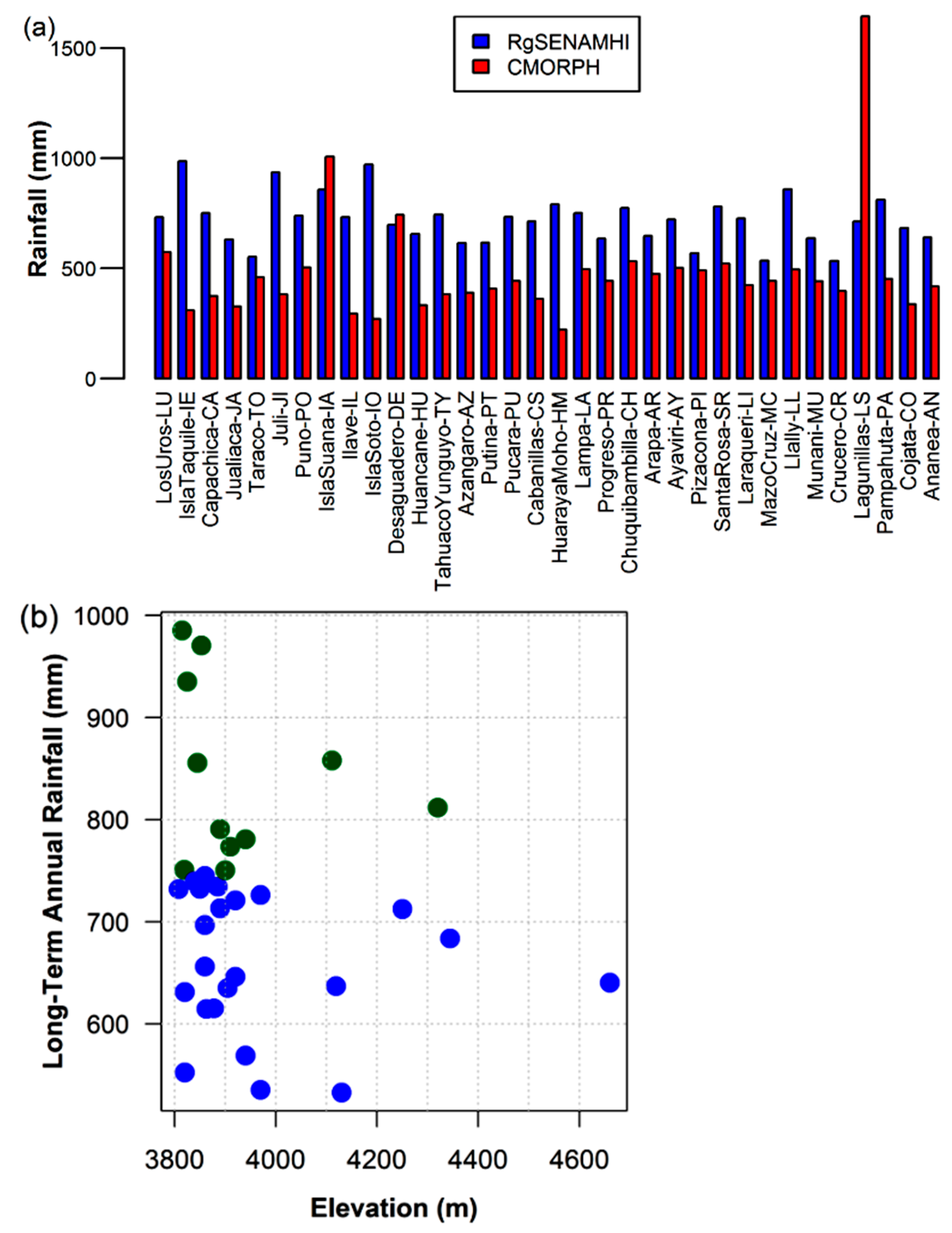
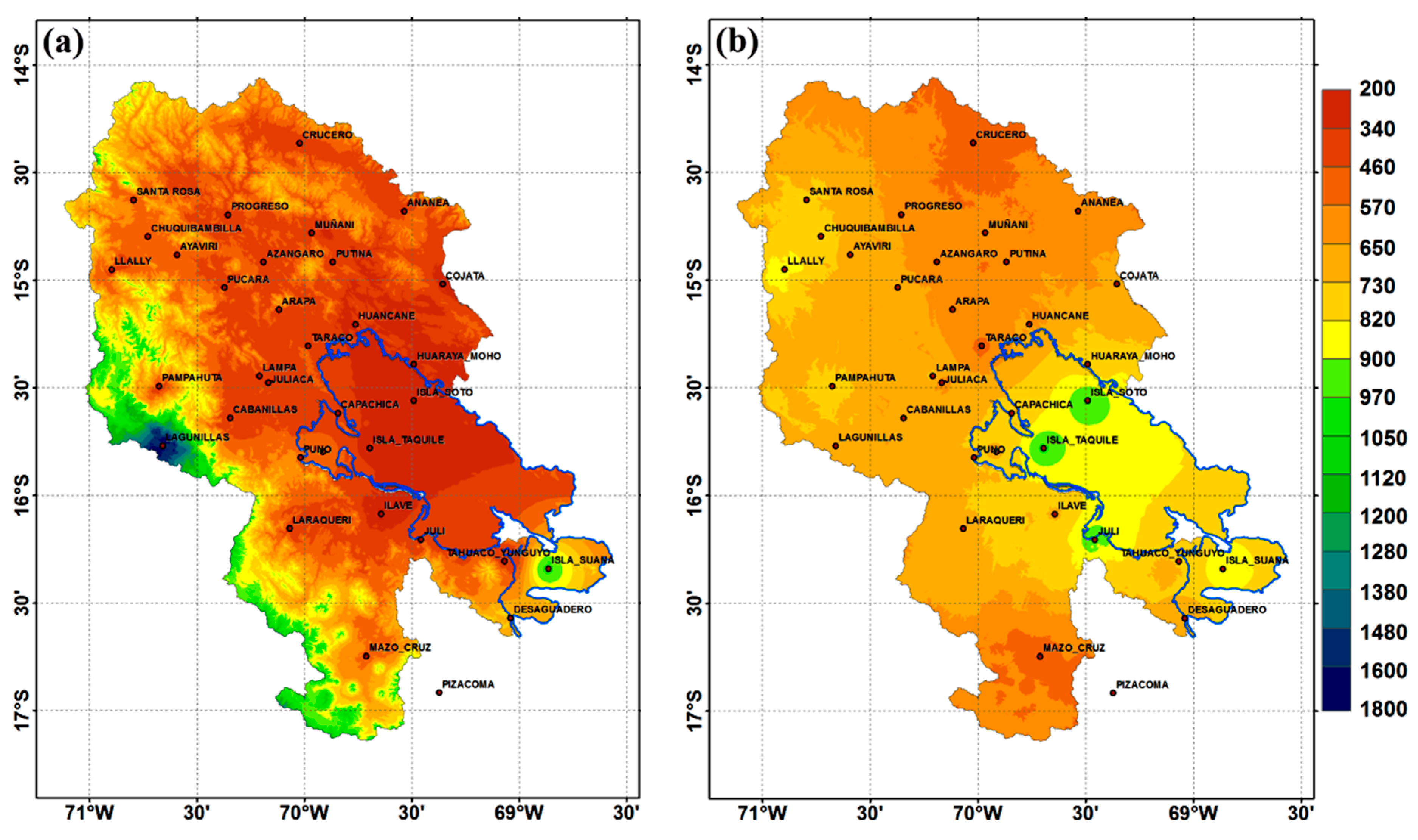
4.1. Point-to-Grid Comparison

The CMORPH rainfall estimates were aggregated to monthly and annual temporal intervals. The RgSENAMHI and the extracted CMORPH for all 34 stations are depicted for the three standard statistical techniques in Figure 3a–c.
As shown in Figure 3a, the monthly CMORPH have strong and weak correlations with the RgSENAMHI. For the CMORPH, the coefficient of determination ranges from a maximum of 0.75 (Chuquibambilla–CH station) to a minimum value of 0.39 (Lagunillas–LS station). On average, 43% of the total RgSENAMHI variation was explained by the CMORPH. In Figure 4, we show the relationships of the CMORPH with RgSENAMHI in the LTb. Over the southeastern and northern LTb, the time series of the CMORPH were positively correlated with RgSENAMHI data and negatively correlated in the central and southern LTb. For some regions (e.g., Lagunillas), the correlation coefficients were statistically insignificant.
The bias calculated (Figure 3b) for the CMORPH and RgSENAMHI ranges from 0.28 to 0.86. The CMORPH was consistent in underestimating the RgSENAMHI; on average, it underestimated it by 60%. The CMORPH overestimated three stations (Lagunillas–LS, Isla Suana–IA, and Desaguadero-DO, marked in green circles in Figure 3b), and it had the largest standard deviation of bias indicating the spread of the bias between stations. These stations registered average values of 150 mm of rainfall during dry season months (June, July, and August), that increased the annual cumulative average (Figure 5a). The root mean square error in Figure 3c gives similar trends as in Figure 3a. Figure 3c shows that the RMSE values of some stations are between the maximum and the average. This shows that CMORPH data would overestimate precipitation values, e.g., Lagunillas–LS, Isla Suana-IS, and Lampa–LA.
Stations likely affected by convective rainfall (11 stations, marked in green circles in Figure 5b) have a better correlation coefficient and a smaller RMSE than the stations likely affected by a combination of orography and convective precipitation (23 stations, marked in blue circles in Figure 5b). The bias also indicated that stations likely affected by both convective and orographic rainfall will have a higher bias than the stations likely affected by convective rain only. This is in agreement with the findings of [54] where, 16 stations registered a higher bias, concluding that this would be affected because of the orographic lifting of moist air that leads to precipitation, while the cloud-top temperature is still relatively warm.

4.2. Areal Comparison

To make a more realistic comparison, areal RgSENAMHI was compared with the areal CMORPH for the LTb, through the methodology of linear multiple regression, where the topography variable was included in rainfall spatial distribution (Figure 6a–d). We first compared the mean cumulative annual precipitation rate. Figure 5a,b show the distributions of precipitation rates of 2002–2013, derived from the CMORPH and RgSENAMHI, respectively. The CMORPH stations with values recorded in the dry season show a precipitation maximum over three regions: the southern, western, and southwestern LTb (Figure 6a).
Note that the magnitude and extent of the maximum of the RgSENAMHI exist mainly over Lake Titicaca (Figure 6b). The results reflect the nonuniform precipitation characteristics over the selected region well, which is under the combined influence of orographic and convective precipitation, exhibiting remarkable accordance in the major precipitation patterns due to the presence of the Andes Mountain range. During the summers (December, January, and February) of 2002–2013, the distributions of mean precipitation rates derived from the CMORPH and RgSENAMHI indicate decreases from the northwest to the southeast (Figure 6c) and from the north to the south (Figure 6d). In addition, there is a minimum center of CMORPH estimates over the northeastern LTb, where some stations are located on the east slope of Chaupi Orco Mountain. The CMORPH can identify this foehn effect, due to its high spatial resolution. Moist air brought by the low-level jet mostly falls as rainfall on the windward slope, causing insufficient water vapor supply on the lee side, which is generated by the presence of the mountain chain that acts as a natural barrier, restricting the entry of moisture from the Amazon. These results were also obtained by Zhang et al. [5], who used satellite data from the CMORPH and TRMM on the South and East Asia region. Overall, the CMORPH precipitation pattern is more similar to the RgSENAMHI precipitation pattern, especially over the northeastern and southeastern LTb.
The areal bias computed (Figure 7a,b), which represents the difference between the CMORPH and RgSENMAHI, presented a high underestimation percentage of the annual cumulative average rainfall (300% on average), while for the summer precipitation, the areal bias was underestimated by an average of 78%. The bias for the CMORPH both for the annual cycle of precipitation and austral summer is not constant; it overestimated for Lagunillas by 930% and underestimated for Isla Soto by 700% (Figure 7a). The summer precipitation bias map (Figure 7b) indicates that the CMORPH consistently underestimated the RgSENAMHI for Isla Soto and Lagunillas by 156 and 38%, respectively. This means that the CMORPH data have limitations in their way of representing small-scale precipitation systems and isolated deep convection. This suggests the difficulties of capturing orographic enhancement of rainfall associated with cap clouds and feeder–seeder cloud interactions over ridges.

4.3. Diurnal Cycle of Precipitation Using Data from CMORPH

We examined the characteristics of the summer diurnal precipitation cycle in detail using the high resolution CMORPH data. Figure 8 shows the spatial distribution of the diurnal cycle intensity and phase of summer precipitation (December, January, and February) over Lake Titicaca and its peripheral areas (period 2002–2013), derived from the CMORPH estimates. As shown in Figure 8, over continental areas, the precipitation peaks in the afternoon. The time of precipitation maximum generally occurs near or shortly after the peak surface heating overland, and there is a marked preference for precipitation maximum between 14:00–20:00 LST. This is due to the Altiplano region absorbing more solar radiation during the day [55,56,57], which results in maximum low-level atmospheric instability and moist convection, causing the rainfall peaks in the late afternoon. The predominant southeastern LTb winds propagate the thermal convection activities to the northwest of the LTb, leading to a precipitation maximum during 16:00–17:00 LST over the surrounding terrain northwest of Lake Titicaca (Figure 8e).
Over Lake Titicaca, precipitation peaks generally occur between midnight and sunrise. The maximum precipitation usually occurs during 04:00–06:00 LTS (Figure 8b), especially over the northwest of Lake Titicaca. The WRF model results were compared rather favorably with observations in the SALLJEX simulations [58] that showed that the regions of preferred convergence and vertical motion are consistent with distribution pattern derived from the CMORPH data. Both of these observations are consistent with the studies referenced in Section 1.
During nighttime (Figure 8a,g,h), the thermal gradient between the lake and the surroundings is the main driver for the breeze development over the lake. With the air coming from the continent to the lake, a terrestrial breeze front is formed with upward motion on the lake. In some cases, it is possible to observe cloud formation and precipitation core estimates.
Figure 9 shows the diurnal cycle of the region’s average summer precipitation from seven selected regions around the LTb (See Figure 1 for the locations on the map) derived from the CMORPH. Region 1—Puno; Region 2—Santa Rosa; Region 3—Crucero; Region 4—Cabanillas; Region 5—Isla Suana; Region 6—Arapa; and Region 7—Isla Soto. In particular, in the regions 3, 5, and 7, we observed an obvious semidiurnal cycle. For the other four regions, the diurnal cycle was dominant, and the peaks were consistent with the previous phase results. When we compared Figure 9a with Figure 10, the results suggest that the CMORPH captured the diurnal phase of convective precipitation. The time of the maximum peak is about 1–2 h earlier that the RgSENAMHI-Puno. It is around 18:00 LST.
This result suggests that the main pattern of the diurnal cycle of precipitation is consistent with previous studies [5,14,46,47]. On the other hand, the high resolution of the CMORPH data used here shows more significant regional differences when compared to previous studies, such as a less coherent phase pattern over certain regions (regions 3, 5, and 7). The remarkable spatial dependence in the DCP over the LTb is clear; there are effects of orography and heterogeneous land–surface impacts on convective development, and the surface temperature differences resulting from the diurnal variation of solar heating and the inhomogeneous underlying surface may induce local circulation through thermal and dynamic effects [59], thus ultimately generating the DCP.
The characteristics of the diurnal precipitation cycle over Lake Titicaca and its vicinity may result from the local circulation influenced by the gradient thermal between the lake and the complex terrain. The slope mountain effects on the available radiant energy [56,57], orographic moisture blockage over the LTb, and the corresponding local advection processes impact the DCP.
In this matter, there are many other factors affecting the regional features of the DCP, such as the regional conditions of water vapor coming from Lake Titicaca. Understanding how this mechanism influences the DCP over the surrounding terrain remains to be further investigated.

5. Conclusions

Rainfall estimation accuracy is very important for LTb’s agricultural growth and safety from natural disasters related to flooding and droughts [1,38,59,60]. In this study, our aim was to assess the accuracy of the CMORPH satellite-rainfall product over the Lake Titicaca basin. This basin is the principal source of the Desaguadero River. The assessment was conducted at the highest spatial resolution of the product (8 × 8 km2) and at several temporal scales (hourly, seasonally, and annually) between January 2002 and December 2013, and an evaluation was made possible through the use of 34 sets of rain gauges available in the region. We used graphical techniques and several statistical metrics to examine the product accuracy. Results, which are displayed in terms of spatial maps, should be interpreted with particular care for parts of the basin where there are few or no rain gauges, especially over the southwestern LTb. The major conclusions can be drawn based on the results summarized as follows:
  • The CMORPH estimates exhibit remarkable accordance with the RgSENAMHI data in terms of their precipitation patterns and captured daily rainfall frequency better that rainfall amounts over the LTb. The precipitation maximum mainly exist over two regions: Lake Titicaca and the surrounding terrain. However, the magnitude and extent of the maximum of the CMORPH rainfall were smaller than those of the RgSENAMHI rainfall. On the other hand, rainfall occurrences are underestimated over most of the LTb, but there are differences over some areas (e.g., Lagunillas, Isla Suana, and Desaguaderos stations) where rainfall is overestimated.
  • Precipitation over our study domain showed diurnal cycles with obvious regional differences. Over the surrounding lake area, the plateau, and high mountain areas, precipitation peaks are in the late afternoon, while over low areas, such as the valleys (near to lake) and Lake Titicaca, it peaks around midnight to early morning. This result suggests that the diurnal cycle of precipitation is closely related to the local circulation resulting from solar radiation and the complex orography.
  • The bias underestimation was observed over most of the LTb areas and overestimation (e.g., Lagunillas, Isla Suana, and Desaguadero stations). The total bias decreases when approaching the lake attaining its minimum value over the mountains [4,5]. In addition, the high resolution of the CMORPH data can depict finer regional details, such as a less coherent phase pattern over a few regions (e.g., Isla Suana).
  • The CMORPH and RgSENAMHI rainfall amounts show weak to moderate correlations (41% and 59%), respectively. Higher correlations were observed over the lake (>0.6). Based on the period and study area, there was a distinct difference between the accuracy of the CMORPH and RgSENAMHI. It was also observed that the accuracy of the CMORPH in the LTb shows large spatial variability [4,5]. On the other hand, efforts should be devoted toward applying spatially and temporally-varying bias correction to the CMORPH product and evaluating the implications of such adjustments for water resource applications in the study area [8].

Author Contributions

E.C.A. and A.J.P.F. analyzed the data; A.J.P.F. contributed materials and analysis tools; E.C.A. wrote the article. All authors have read and agreed to the published version of the manuscript.

Funding

This research publication was sponsored by PROEX/CAPE The second author is supported by Conselho Nacional de Desenvolvimento Científico e Tecnológico (CNPq) under grant 302349/2017-6.

Institutional Review Board Statement

Not applicable.

Informed Consent Statement

Not applicable.

Data Availability Statement

Is excluded.

Acknowledgments

The present work was the result of the master’s thesis financed by Capes (Coordination of Improvement of Higher-Level Personnel), foundation of the Ministry of Education of Brazil.

Conflicts of Interest

The authors declare no conflict of interest.

Abbreviations

The following abbreviations are used in this manuscript:
CMORPHCPC MORPHing technique
LTbLake Titicaca basin
LSTLocal Solar Time
RgSENAMHIRain gauge SENAMHI

References

  1. Canedo, C.; Pillco, R.Z.; Berndtsson, R. Role of Hydrological Studies for the Develompent of the TDPS System. Water 2016, 8, 144. [Google Scholar] [CrossRef] [Green Version]
  2. Li, J.; Heap, A.D. Spatial Interpolation Methods: A Review for Environmental Scientists; Geoscience Australia: Canberra, Australia, 2008. Available online: https://www.ga.gov.au/corporate_data/68229/Rec2008_023.pdf (accessed on 20 July 2019).
  3. Scheel, M.L.M.; Rohrer, M.; Huggel, C.; Santos Villar, D.; Silvestre, E.; Huffman, G.J. Evaluation of TRMM Multi-satellite Precipitation Analysis (TMPA) performance in the Central Andes region and its dependency on spatial and temporal resolution. Hydrol. Earth Syst. Sci. 2011, 15, 2649–2663. [Google Scholar] [CrossRef] [Green Version]
  4. Haile, A.T.; Yan, T.; Habib, E. Accuracy of the CMORPH satellite-rainfall product over Lake Tana Basin in Eastern Africa. Atmos. Res. 2015, 163, 177–187. [Google Scholar] [CrossRef] [Green Version]
  5. Zhang, X.-X.; Bi, X.-Q.; Kong, X.-H. Observed Diurnal Cycle of Summer Precipitation over South Asia and East Asia Based on CMORPH and TRMM Satellite Data. Atmos. Ocean. Sci. Lett. 2015, 8, 201–207. [Google Scholar] [CrossRef]
  6. Dinku, T.; Connor, S.J.; Ceccato, P. Comparation of CMORPH and TRMM-3B42 over Mountainous Regions of Africa and South America. In Satellite Rainfall Applications for Surface Hydrology; Gebremichael, M., Hossain, F., Eds.; Springer: Dordrecht, The Netherlands, 2009. [Google Scholar] [CrossRef]
  7. Pereira, F.A.J.; Carbone, R.E.; Janowiak, J.E.; Arkin, P.; Joyce, R.; Hallak, R.; Ramos, C.G.M. Satellite rainfall estimates over South America—Possible applicability to the water management of large watersheds. J. Am. Water Resour. Assoc. 2010, 46, 344–360. [Google Scholar] [CrossRef]
  8. Pereira, F.A.J.; Vemado, F.; Vemado, G.; Gomes, V.R.F.A.; Do Carmo, G.L.; Irineu, C.R.; Dos Santos, C.C.; Sampaio, L.E.S.; Fischer, G.M.; Tadashi, O.A.; et al. A Step towards Integrating CMORPH Precipitation Estimation with Rain Gauge Measurements. Adv. Meteorol. 2018, 2018, 1–24. [Google Scholar] [CrossRef]
  9. Ruiz, J.J. Evaluation of different methodologies for precipitation estimates calibration-cmorph-over South America. Rev. Bras. Meteorol. 2009, 24, 4. [Google Scholar] [CrossRef]
  10. Sapriano, M.R.P.; Arkin, P.A. An Intercomparison and Validation of High-Resolution Satellite Precipitation Estimates with 3-Hourly Gauge Data. J. Hydrometeorol. 2019, 10, 149–166. [Google Scholar] [CrossRef]
  11. Dinku, T.; Chidzambwa, S.; Ceccato, P.; Connor, S.J.; Ropelewski, C.F. Validation of high-resolution satellite rainfall products over complex terrain. Int. J. Remote Sens. 2008, 29, 4097–4110. [Google Scholar] [CrossRef]
  12. Satgé, F.; Bonnet, M.-P.; Gosset, M.; Molina, J.; Yuque, L.W.H.; Pillco, Z.R.; Timouk, F.; Garnier, J. Assessment of satellite rainfall products over the Andean plateau. Atmos. Res. 2016, 167, 1–14. [Google Scholar] [CrossRef]
  13. Satgé, F.; Ruelland, D.; Bonnet, M.-P.; Gosset, M.; Molina, J.; Pillco, Z.R. Consistency of satellite-based precipitation products in space and over time compared with gauge observations and snow-hydrological modelling in the Lake Titicaca region. Hydrol. Earth Syst. Sci. 2019, 23, 595–619. [Google Scholar] [CrossRef] [Green Version]
  14. Dai, A.; Lin, X.; Hsu, K.-L. The frequency, intensity, and diurnal cycle of precipitation in surface and satellite observations over low- and mid-latitudes. Clim. Dyn. 2007, 29, 727–744. [Google Scholar] [CrossRef]
  15. Janowiak, J.E.; Arkin, P.A.; Morrissey, M. An examination of the diurnal cycle in oceanic tropical rainfall using satellite and in situ data. Mon. Weather. Rev. 1994, 122, 2296–2311. [Google Scholar] [CrossRef] [Green Version]
  16. Chang, A.T.C.; Chiu, L.S.; Yang, G. Diurnal cycle of oceanic precipitation from SSM/I data. Mon. Weather. Rev. 1995, 123, 3371–3380. [Google Scholar] [CrossRef] [Green Version]
  17. Sorooshian, S.; Gao, X.; Maddox, R.A.; Hon, Y.; Imam, B. Diurnal variability of tropical rainfall retrieved from combined GOES and TRMM satellite information. J. Clim. 2002, 15, 983–1001. [Google Scholar] [CrossRef] [Green Version]
  18. Nesbitt, S.W.; Zipser, E.J. The diurnal cycle of rainfall and convective intensity according to three years of TRMM measurements. J. Clim. 2003, 16, 1456–1475. [Google Scholar] [CrossRef] [Green Version]
  19. Bowman, K.P.; Collier, J.C.; North, G.R.; Wu, Q.Y.; Ha, E.H.; Hardin, J. Diurnal cycle of tropical precipitation in Tropical Rainfall Measuring Mission (TRMM) satellite and ocean buoy rain gauge data. J. Geophys. Res. 2005, 110, D21104. [Google Scholar] [CrossRef] [Green Version]
  20. Hong, Y.; Hsu, K.L.; Sorooshian, S.; Gao, X.G. Improved representation of diurnal variability of rainfall retrieved from the Tropical Rainfall Measurement Mission Microwave Imager adjusted Precipitation Estimation From Remotely Sensed Information Using Artificial Neural Networks (PERSIANN) system. J. Geophys. Res. 2005, 110, D06102. [Google Scholar] [CrossRef] [Green Version]
  21. Yang, S.; Smith, E.A. Mechanisms for diurnal variability of global tropical rainfall observed from TRMM. J. Clim. 2006, 19, 5190–5226. [Google Scholar] [CrossRef] [Green Version]
  22. Hur, J.; Srivatsan, V.R.; Ngoc, S.N.; Shie-Yui, L. Evaluation of High-Resolution Satellite rainfall data over Singapure. Procedia Eng. 2016, 154, 158–167. [Google Scholar] [CrossRef] [Green Version]
  23. Shang, H.; Letu, H.; Nakajima, T.Y.; Wang, Z.; Ma, R.; Wang, T.; Lei, Y.; Ji, D.; Li, S.; Shi, J. Diurnal cycle and seasonal variation of cloud cover the Tibetan Plateau as determined from Himawari-8 new-generation geostationary satellite data. Sci. Rep. 2018, 8, 1105. [Google Scholar] [CrossRef] [PubMed]
  24. Wang, G.; Zhang, P.; Liang, L.; Zhang, S. Evaluation of precipitation from CMORPH, GPCP-2, TRMM 3B43, GPCC and ITPCAS with ground-based measurements in the Qinling-Daba Mountains, China. PLoS ONE 2017, 12, e0185147. [Google Scholar] [CrossRef] [PubMed] [Green Version]
  25. Dai, A. Global Precipitation and Thunderstorm Frequencies. Part I: Seasonal and Interannual Variations. J. Clim. 2000, 14, 1092–1111. [Google Scholar] [CrossRef]
  26. Du, Y.; Rotunno, R. Diurnal Cycle of Rainfall and Winds near the South Coast of China. Am. Meteorol. Soc. 2018, 75, 2065–2082. [Google Scholar] [CrossRef]
  27. Watters, D.; Battaglia, A. The Summertime Diurnal Cycle of Precipitation Derived from IMERG. Remote Sens. 2019, 11, 1781. [Google Scholar] [CrossRef] [Green Version]
  28. Garreaud, R.; Vuille, M.; Clement, A. The climate of the Altiplano: Observed current conditions and mechanisms of past changes. Palaeogeogr. Palaeoclimatol. Palaeoecol. 2003, 194, 5–22. [Google Scholar] [CrossRef] [Green Version]
  29. Sato, T. Mechanism of Orographic Precipitation around the Meghalaya Plateau Associated with Intraseasonal Oscillation and the Diurnal Cycle. Mon. Weather Rev. 2013, 141, 3049–3064. [Google Scholar] [CrossRef] [Green Version]
  30. Minder, J.; Letcher, T.W. The Evolution of Lake-Effect Convection during Landfall and Orographic Uplift as Observerd by Profiling Radars. Mon. Weather Rev. 2015, 143, 4422–4442. [Google Scholar] [CrossRef]
  31. Veals, P.G.; Steenburgh, W.J.; Campell, L.S. Factors Affeting the Inland and Orographic Enhancement of Lake-Effect Precipitation over the Tug Hill Plateau. Mon. Weather Rev. 2018, 146, 1745–1762. [Google Scholar] [CrossRef]
  32. Nicholson, S.E.; Hartman, A.T.; Klaust, D.A. On the Diurnal Cycle of Rainfall and Convection over Lake Victoria and Its Catchment. Part II: Meteorological Factors in the Diurnal and Seasonal Cycles. J. Hydrometeorol. 2021, 22, 3049–3064. [Google Scholar] [CrossRef]
  33. Garreaud, R. Intraseasonal Variability of Misture and Rainfall over the South American Altiplano. Mon. Weather Rev. 2000, 128, 3337–3346. [Google Scholar]
  34. Villue, M.; Keimig, F. Interannual Variability of Summertime Convective Cloudiness and Precipitation in the Central Derived from ISCCP-B3 Data. J. Clim. 2004, 17, 3334–3348. [Google Scholar] [CrossRef] [Green Version]
  35. OEA (Organización de los Estados Americanos)/PNUMA (Programa de las Naciones Unidas para el Medio Ambiente). Diagnóstico Ambiental del Sistema Titicaca-Desaguadero-Poopó-Salar de Copaisa (Sistema TDPS) Bolivia-Perú; OEA: Washington, DC, USA, 1996; p. 192. [Google Scholar]
  36. Heidinger, H.; Yarlequé, C.; Posadas, A.; Quiroz, R. TRMM rainfall correction over the Andean Plateau using wavelet multi-resolution analysis. Int. J. Remote Sens. 2012, 33, 4583–4602. [Google Scholar] [CrossRef]
  37. Torre-Batlló, J.; Martí-Cardona, B.; Pillco-Zolá, R. Mapping long-term evapotranspiration losses in the catchment of the shrinking Lake Poopó. Hydrol. Earth Syst. Sci. 2019. preprint. [Google Scholar] [CrossRef] [Green Version]
  38. Zamuriano, M.; Martynov, A.; Panziera, L.; Bronnimann, S. Characteristics of a Hailstorm over the Andean La Paz Valley. Nat. Hazards Earth Syst. Sci. 2019. preprint. [Google Scholar] [CrossRef]
  39. Blacutt, L.A.; Herdies, D.L.; De Gonçalves, L.G.G.; Vila, D.A.; Andrade, M. Precipitation comparison for the CFSR, MERRA, TRMM3B42 and Combined Scheme datasets in Bolivia. Atmos. Res. 2015, 163, 117–131. [Google Scholar] [CrossRef] [Green Version]
  40. Gebere, S.B.; Alamirew, T.; Merkel, B.J. Performance of High-Resolution Satellite Rainfall Products over Data Scarse Parts of Eastern Ethiopia. Remote Sens. 2015, 7, 11639–11663. [Google Scholar] [CrossRef] [Green Version]
  41. Joyce, R.J.; Janowiak, J.E.; Arkin, P.A.; Xie, P. CMORPH: A Method that Produces Global Precipitation Estimates from Passive Microware and Infrared Data at High Spatial and Temporal Resolution. J. Hydrometeorol. 2004, 5, 487–503. [Google Scholar] [CrossRef]
  42. Joice, R.J.; Xie, P.; Yarosh, Y.; Janowiak, J.E.; Arkin, P.A. CMORPH: A “Morphing” Approach for High Resolution Precipitation Product Generation. In Satellite Rainfall Applications for Surface Hydrology; Springer: Dordrecht, The Netherlands, 2009. [Google Scholar] [CrossRef]
  43. Rais, A.F.; Yunita, R. Main Diurnal Cycle Pattern of Rainfall in East Java. AIP Conf. Proc. 2017, 1876, 020057. [Google Scholar] [CrossRef] [Green Version]
  44. Zhu, L.; Meng, Z.; Zhang, F.; Markowski, P.M. The influence of sea and land-breeze circulations on the diurna variability in preciptation over a tropical island. Atmos. Chem. Phys. 2017, 17, 13213–13232. [Google Scholar] [CrossRef] [Green Version]
  45. Hussain, Y.; Satgé, H.; Hussain, M.B.; Martinez-Carvajal, H.; Bonnet, M.-P.; Cárdenas-Soto, M.; Roig, H.L.; Akther, G. Performance of CMOPRH, TMPA, and PERSIANN rainfall datasets oven plain, mountainous and glacial regions of Pakistan. Theor. Appl. Clim. 2018, 131, 1119–1132. [Google Scholar] [CrossRef]
  46. Janowiak, J.E.; Kousky, V.E.; Joyce, R.J. Diurnal cycle of precipitation determined from the CMORPH high spatial and temporal resolution global precipitation analyses. J. Geophys. Res. 2005, 110, D23105. [Google Scholar] [CrossRef] [Green Version]
  47. Giles, J.A.; Ruscia, R.C.; Menéndez, C.G. The diurnal cycle of precipitation over South America represented by five gridded datasets. Int. J. Climatol. 2019, 40, 1–19. [Google Scholar] [CrossRef]
  48. Trinh-Tuan, L.; Matsumoto, J.; Ngo-Duc, T.; Nodzu, M.I.; Inoue, T. Evaluation of satellite precipitation products over Central Vietnan. Prog. Earth Planet. Sci. 2019, 6, 54. [Google Scholar] [CrossRef] [Green Version]
  49. TDPS: Climatología del Sistema de los Lagos Titicaca, Desaguadero, Poopó y Salares Coipasa y Uyuni (TDPS); Comisión de Comunidades de Europeas, Repúblicas del Perú y Bolivia: La Paz, Bolivia, 1993.
  50. Revollo, M.M. Management issues in the Lake Titicaca and Lake Poopo System: Importance of developing a water budget. Lake Reserv. 2001, 6, 225–229. [Google Scholar] [CrossRef]
  51. Roche, M.A.; Bourges, J.; Cortes, J.; Mattos, R. Climatology and hydrology of the Lake Titicaca basin. In Lake Titicaca. A Synthesis of Limnological Knowledge; Dejoux, C., Litis, A., Eds.; Kluwer Academic Publishers: Dordrecht, The Netherlands, 1992; pp. 63–88. [Google Scholar]
  52. Hunziker, S.; Gubler, S.; Calle, J.; Moreno, I.; Andrade, M.; Velarde, F.; Ticona, L.; Carrasco, G.; Castellón, Y.; Oria, C.; et al. Identifying, attributing, and overcoming common data quality is-sues of manned station observations. Int. J. Climatol. 2017, 37, 4131–4145. [Google Scholar] [CrossRef]
  53. Quevedo, K.; Sánchez, K. Comparison of two interpolation methods to estimate air temperature applying geostatistical techniques. Rev. Peru. Geo-Atmos. 2009, 1, 90–107. [Google Scholar]
  54. Worqlul, A.W.; Maathuis, A.; Adem, A.A.; Demissie, S.S.; Langan, S.; Steenhuis, T.S. Comparison of rainfall estimations by TRMM 3B42, MPEG and CFSR with ground-observed data for the Lake Tana basin in Ethiopia. Hydrol. Earth Syst. Sci. 2014, 18, 4871–4881. [Google Scholar] [CrossRef] [Green Version]
  55. Budyko, M.I. Climate and life. In International Geophysics Series; Miller, D.H., Ed.; Academic Press: Cambridge, MA, USA, 1974; Volume 18, 508p. [Google Scholar]
  56. Kato, S.; Loeb, N.G.; Rosse, F.G.; Doelling, D.R.; Rutan, D.A.; Caldwell, T.E.; Yu, L.; Weller, R.A. Surface irradiances consistent with CERES-derived top-of-atmosphere shortwave and longwave irradiances. J. Clim. 2013, 26, 2719–2740. [Google Scholar] [CrossRef]
  57. Gálvez, J.M.; Douglas, M.W. Modulation of rainfall by Lake Titicaca using the WRF Model. In Proceedings of the 8th ICSHMO, Foz do Iguaçu, Brazil, 24–28 April 2006; pp. 745–752. [Google Scholar]
  58. Zaratti, F.; Forno, R.N.; García, J.F. Erythemally weighted UV variations at two high-altitude locations. J. Geophys. Res. 2003, 108. [Google Scholar] [CrossRef]
  59. Canedo, R.C.; Hochrainer-Stigler, S.; Pflug, G.; Condori, B.; Berndtsson, R. Early warning and drought risk assessment for the Bolivian Altiplano agriculture using high resolution satellite imagery data. Nat. Hazards Earth Syst. Sci. 2018. preprint. [Google Scholar] [CrossRef] [Green Version]
  60. Canedo, R.C.; Hochrainer -Stigler, S.; Pflug, G.; Condori, B.; Berndtsson, R. Drought risk in the Bolivian Altiplano associated with El Niño Southern Oscillation using satellite imagery data. Nat. Hazards Earth Syst. Sci. 2019, 21, 995–1010. [Google Scholar] [CrossRef]
Figure 1. Study site of Lake Titicaca basin, Peru, showing the locations of rain gauge stations (represented by stars). The gray color scale represents elevation over the basin. The circles represent the subregions studied: Region 1—Puno (70°01′18″–69°44′55″ W, 15°58′28″–15°43′13″ S); Region 2—Santa Rosa (70°53′20″–70°33′54″ W, 14°39′35″–14°58′15″ S); Region 3—Crucero (70°03′47″–69°46′15″ W, 14°31′12″–14°47′35″ S); Region 4—Cabanillas (70°46′05″–70°27′02″ W, 15°34′51″–15°53′31″ S); Region 5—Isla Suana (68°59′27″–68°39′56″ W, 16°13′59″–16°33′32″ S); Region 6—Arapa (70°12′32″–69°55′16″ W, 15°05′02″–15°21′56″ S); Region 7—Isla Soto (68°28′43″–69°10′49″ W, 15°38′39″–15°55′48″ S).
Atmosphere 13 00601 g001
Figure 2. Average monthly gauged rainfall distribution of selected stations in the Lake Titicaca basin (from 2002 to 2013).
Atmosphere 13 00601 g002
Figure 3. (a) R2 of CMORPH compared with 34 RgSENAMHI in the LTb. (b) Bias of CMORPH compared with 34 RgSENAMHI in the LTb. (c) RMSE of CMORPH compared with 34 RgSENAMHI in the LTb.
Atmosphere 13 00601 g003aAtmosphere 13 00601 g003b
Figure 4. Pearson correlation coefficients (Pearson) of CMORPH with RgSENAMHI for the period 2002–2013.
Atmosphere 13 00601 g004
Figure 5. (a) Annual average rainfall CMORPH and RgSENAMHI (2002–2013) of selected stations in the Lake Titicaca basin. (b) Elevation vs. long-term annual average rainfall relations in the Lake Titicaca basin (34 stations from 2002 to 2013).
Atmosphere 13 00601 g005
Figure 6. Spatial distribution of the annual and summer season precipitation (2002–2013): (a) CMORPH, (b) observed data for the summer precipitation (DJF), (c) CMORPH, and (d) observed data. The scale in colors represents the precipitation in millimeters (mm). Vertical axis indicates the latitudes, and the horizontal axis refers to the lengths, both in degrees (°).
Atmosphere 13 00601 g006aAtmosphere 13 00601 g006b
Figure 7. Bias spatialization map for the annual precipitation cycle (a) and for the summer precipitation (b). Period 2002–2013. Scale in colors represents the underestimation or overestimation of CMORPH compared to RgSENAMHI.
Atmosphere 13 00601 g007
Figure 8. Spatial distribution of the average rainfall accumulation field obtained from the CMORPH data, period 2002–2013. Color scale represents precipitation in millimeters (mm/hr). The diurnal cycle of precipitation is represented in local solar time (LST). Vertical axis indicates the latitudes, and the horizontal axis refers to the lengths, both in degrees (°). The white boxes (R1–R7) are the regions selected for the analysis. (a) 0–1 Local Solar Time; (b) 3–4 Local Solar Time; (c) 6–7 Local Solar Time; (d) 9–10 Local Solar Time; (e) 12–13 Local Solar Time; (f) 15–16 Local Solar Time; (g) 18–19 Local Solar Time; (h) 21–22 Local Solar Time.
Atmosphere 13 00601 g008aAtmosphere 13 00601 g008b
Figure 9. Mean diurnal cycle of summer precipitation at seven selected regions. CMORPH (thin gray solid line indicates 2002–2013). The abscissa represents the diurnal cycle phase (LST), and the ordinate represents the region’s average precipitation rate (units: mm d−1). (a) Region Puno; (b) Region Santa Rosa; (c) Region Crucero; (d) Region Cabanillas; (e) Region Isla Suana; (f) Region Arapa; (g) Region Isla Soto.
Atmosphere 13 00601 g009aAtmosphere 13 00601 g009b
Figure 10. Mean diurnal cycle of summer precipitation at the automatic weather station (Puno). RgSENAMHI-Puno (thin gray solid line indicates 2014–2018). The abscissa represents the diurnal cycle phase (LST), and the ordinate represents the region’s average precipitation rate (units:mm d−1).
Atmosphere 13 00601 g010
Table 1. Summary of precipitation data sets used in this study.
Dataset Name
(Reference)
Spatial–Temporal
Resolution and Coverage
Data Sources and Merging MethodOnline Documentation
CMORPH
(Joyce et al., 2004) [41]
0.07275° grid, 60° S–60° N, 180° W–180° E; 30 min, 12/2002-present.Microwave estimates from the DMSP 13, 14, and 15 (SSM/I); the NOAA-15, 16, and 17 (AMSU-B); and the TRMM (TMI) satellites are propagated by motion vectors derived from geostationary satellite infrared data.(http://www.cpc.ncep.noaa.gov/products/janowiak/cmorph_description.html). Accessed on 10 September 2019
Rain gauges (SENAMHI)
(Hunziker et al., 2017) [52]
14° S–18° S, 71° W–69° W
1964–2013
Daily reports from 34 rain gauges were used to derive the gridded data.(http://www.geography.unibe.ch/research/climatology group/research_projects/decade/index_eng.html). Accessed on 21 July 2019
Publisher’s Note: MDPI stays neutral with regard to jurisdictional claims in published maps and institutional affiliations.

