Abstract
Turbulence kinetic energy (TKE) schemes are routinely used for turbulence parameterization in numerical weather prediction models. A key component of these schemes is the so-called turbulence length scale. Novel scale-aware, budget-based diagnostics that account for the cross-scale transfer of variances are used to evaluate the performance of selected turbulence length scale formulations in the gray zone of turbulence. The diagnostics are computed using the coarse-graining method on high resolution large eddy simulation data for selected idealized cases. The vertical profiles and the temporal evolution of the turbulence length scales are analyzed. Additionally, the local normalized root mean square error and a non-local three-component technique tailored specifically to the turbulence length scale profiles are used for the evaluation. Based on our analyses, we recommend using turbulence length-scale formulations that depend not only on the boundary layer height, but also on the TKE and stratification. Such formulations are able to perform satisfactorily in different flow regimes, but their scale-awareness is still limited. Only the Honnert et al. formulation shows a stronger scale-awareness thanks to its cut-off relationship in the gray zone. However, in contrast to the turbulence length scale diagnostics, its resolution dependence does not change with height.
1. Introduction
Turbulent motions in the atmosphere occur on a range of different scales, from millimeter to kilometer scales [1,2]. As some turbulent motions occur on scales that are always smaller than the resolution of an atmospheric model, basically all atmospheric models require a turbulence parameterization to account for the influence of sub-grid-scale turbulence. The level to which the turbulent flow is parameterized is thus dependent on the resolution of the model. In numerical weather prediction (NWP) and global circulation (GC) models, all turbulent motions, including both large and small eddies, are parameterized. However, in large-eddy simulation (LES) models, only the isotropic turbulent eddies (the smaller eddies) need to be parameterized, because the energy-containing anisotropic turbulent eddies (the larger eddies) are resolved in LES [1,3].
The parameterization of turbulence in models with a resolution between the classical NWP/GC and the LES models is naturally also required, but it is more difficult. This is because the anisotropic turbulent eddies are already partly resolved, and only the unresolved part of the large eddies needs to be parameterized. In this gray zone of turbulence, some classical NWP assumptions need to be revisited [4,5,6]. We focus in this paper particularly on the fact that the net sub-grid cross-scale transfer of turbulence kinetic energy (TKE) is not zero anymore in the gray zone [1].
In order to account for the influence of the cross-scale transfer of TKE, Reference [3] proposed a modification of the turbulence length scale in TKE turbulence schemes. The turbulence length scale is one of the key components in TKE turbulence schemes. Primarily, the turbulence length scale is used to parameterize the viscous dissipation in the prognostic TKE equation. Consequently, the primary output of a turbulence scheme, the vertical turbulent fluxes, are directly affected by the turbulence length scale (see [3,7] for more details). The modifications of the turbulence length scale should lead to a scale-aware formulation of the turbulence length scale, which would enable a better representation of turbulence in the gray zone.
The reference for such a new formulation is a scale-aware diagnostic, where the turbulence length scale is defined through the viscous dissipation of TKE. The TKE dissipation term is calculated from the TKE budget using high-resolution LES data. To obtain the length scale at different resolutions, a coarse-graining method is used on the LES data (averaging over sub-domains of different sizes) [3].
While this TKE-based turbulence length scale diagnostic is accurate in most situations, the use of a TKE budget faces a potential problem when gravity waves are present in and above the atmospheric boundary layer (ABL). Specifically, the velocity fluctuations in the LES data cannot be easily separated between turbulence and wave kinetic energy [2]. In the presence of gravity waves, the TKE can be over-estimated, which yields unrealistic values of the turbulence length scale [3]. This problem can be partly avoided if the length scale is diagnosed from the budgets of the following scalar variances: liquid water potential temperature variance and total specific water content variance. Therefore, we also extend the budget-based diagnostic to scalar variances in this paper.
All three diagnostics are then used for the evaluation of several existing algebraic formulations: the height-dependent Blackadar (1962) [8] and Bastak Duran et al. (2018) [9] formulations, the TKE-dependent Bougeault and Lacarrere (1989) [10] and Honnert et al. (2021) [11] formulations, and the combined Nakanishi and Niino (2009) [12,13] formulation. This particular set represents the most frequently used algebraic turbulence length scale formulations in NWP models. The evaluation is performed for several idealized cases, covering different atmospheric boundary layer conditions.
The paper is organized as follows. Section 2 gives a detailed description of the different budget-based turbulence length scale diagnostics and algebraic formulations, along with a description of the LES model used to simulate a variety of different boundary layer cases. The main results of the study are shown in Section 3, looking in particular at the scale dependence of the budget-based diagnostics, the evaluation of the algebraic turbulence length scale formulations, and the temporal development of the turbulence length scale over the simulated time period. Finally, a summary of the study’s findings along with the main conclusions are found in Section 4.
2. Formulations and Methods
2.1. Turbulence Length Scale Diagnostics
In this study, we evaluate existing algebraic turbulence length scale formulations using turbulence length scale diagnostics computed from coarse-grained LES data (see [3]). Two sets of diagnostics are used for this purpose.
First, the turbulence length scale is diagnosed without consideration of the transfer of TKE or scalar variances across scales. The turbulence length scales are derived from the definition of the viscous dissipation term in the prognostic equations for the TKE and from the definitions of the molecular dissipation terms for the variance of the liquid water potential temperature, , or the total specific water content, (see [3,9] for more details):
where the operator denotes an average over a horizontal sub-domain of size (equivalent to a horizontal grid box in NWP) and over time (in our case over 1 h; see Section 2.3), and the fluctuations from this average are denoted with :
where stands for any relevant quantity, and the average over all sub-domains with size is denoted by (see [3] for more details about the LES coarse graining). , , and are the sub-grid scale TKE, the variance of , and the variance of for sub-domains with size (corresponding to a NWP computational mesh with a grid spacing of ). , , and are the respective diagnosed turbulence length scales. and are closure constants [14,15]. , , and are the viscous/molecular dissipation rates of the TKE, the variance of , and the variance of in their respective Reynolds-averaged (assuming horizontal homogeneity) prognostic equations (see, e.g., [16]):
where the operator denotes an average over the horizontal domain and in time (in our case over the whole LES domain and 1 h; see Section 2.3), and the fluctuations from this average are denoted with :
x, y, and z are horizontal and vertical coordinates; u, v and w are the corresponding components of the wind velocity; t is the time; p is the atmospheric pressure; is the virtual potential temperature; is a reference virtual potential temperature; is a reference density; and g is the gravitational acceleration. The first terms on the left-hand side in Equations (6)–(8) are the tendency terms. The remaining terms on the left-hand side are the horizontal and vertical advection terms. Please note that under the assumption of horizontal homogeneity, the contribution from the advection terms is equal to zero (see, e.g., [1]). The first terms on the right-hand side represent the vertical turbulent transport. For TKE, the turbulent transport term also includes the pressure correlation term (the last expression). The second terms in Equations (6)–(8) are the shear production term for TKE and the gradient terms for scalar variances. The third term on the right-hand side in Equation (6) is the buoyancy production/destruction term.
Second, the above formulations are extended to account for the transfer of TKE or scalar variances across scales:
where , , and are the effective viscous/molecular dissipation rates of the TKE, the variance of , and the variance of , defined as:
where , , and are the cross-scale transfers at the cutoff scale for TKE, the variance of , and the variance of .
Effective dissipation rates are estimated from the budgets of the corresponding variables for a sub-domain of size (obtained as residuals from all other terms computed from the LES data; see [3]):
2.2. Algebraic Turbulence Length Scale Formulation
Five representative algebraic turbulence length scale formulations are evaluated in this study. The length scales are computed for all sub-domain sizes from the corresponding averaged LES data (see Section 2.1). While all the studied algebraic formulations are dependent on different aspects of the boundary layer, all five share a common height dependence, where the turbulence length scale is proportional to height via the von Karman constant, k, in a neutral surface layer.
2.2.1. Blackadar Formulation
The first algebraic formulation used in this study was proposed by Blackadar (1962) [8] and is referred to as for the remainder of this paper. The mixing length is defined as follows:
where z is the altitude and is an asymptotic parameter set to 150 m for unstable layers and to 30 m for stable layers. It should be noted that was derived from similarity law relationship in neutral stratification. The corresponding length scale for a TKE scheme, , is computed from according to [9,17]:
is a closure constant [7].
2.2.2. Bastak Duran et al. Formulation
The next formulation used in Bastak Duran et al. [9], , is an algebraic formulation derived from [18]:
where is the ABL height, calculated using the bulk Richardson number. The constants , , , and are set to be 350 m, 5.5, 3.0, and 0.02, respectively.
2.2.3. Nakanishi and Niino Formulation
The formulation by Nakanishi and Niino (2009) [12,13], , comprises three different turbulence length scale formulations, , , and :
where and are closure constants and , , and are values used for TKE and scalar variances, respectively. Please note that the introduction of , , and is only required for our evaluation since the formulations for the dissipation terms in [13] differ from the formulation that was used in our turbulence length scale diagnostic (Equations (1)–(3)).
The three length scales considered for are dependent on different aspects of the boundary layer. The first of the three length scales, , is the turbulence length scale within the surface layer. Above the surface layer, the value of increases and therefore becomes less significant in the overall calculation. is computed as follows (Equation (53) in [13]):
where is a stability parameter, is the Monin–Obukhov length, is the friction velocity, and is virtual potential temperature flux at the surface.
The second of the three length scales, , is the length scale that is dependent on the boundary layer height [12,13,19]:
where h is the vertical limit of the simulated domain.
The final length scale, is related to how far a parcel of air, with a given TKE, can travel vertically before the buoyancy force stops the motion:
where N is the Brunt–Väisälä frequency and is a velocity scale (see [13]). is most accurate in stable layers.
2.2.4. Bougeault and Lacarrere Formulation
The Bougeault and Lacarrere [10] length scale, , takes the balance between the TKE and buoyancy into account. This length scale is computed by combining the upward and downward free paths, and :
The value of is defined as the movement of a parcel of air with a given TKE in the upward direction until a point where it is stopped by buoyancy effects [10,20]:
The derivation of is similar to , but it is calculated in the opposite direction:
It also has an additional requirement in that the parcel cannot go below the surface. The is scaled similarly to (see Equation (21)) to ensure similarity law relationship near the surface.
2.2.5. Honnert et al. Formulation
The final formulation, derived by Honnert et al. (2021) [11], , is a combination of a non-local turbulence length scale and grid box size:
where and are horizontal sizes of the grid box (in our case sub-domain), is a calibration parameter, and is an extension of by a contribution from shear according to [21]:
where is the vertical wind shear, and are the upward and downward free paths, and is a calibration constant.
2.3. LES Data
A total of five idealized cases with different ABL conditions are used for the evaluation of the turbulence length scale formulations: a continental cumulus case based on data from the Atmospheric Radiation Measurement (ARM) program at the Cloud and Radiation Testbed site in Oklahoma [22], a stratocumulus case with drizzle based on data recorded during the first research flight (RF01) of the second period of the Dynamics and Chemistry of Marine Stratocumulus (DYCOMS-II) campaign [23], a stable boundary layer case based on data from the Global Energy and Water Cycle Experiment (GEWEX) Atmospheric Boundary Layer Study (GABLS1) [24,25], a trade-wind cumulus case from the Barbados Oceanographic and Meteorological Experiment (BOMEX) [26], and a precipitating shallow cumulus case from the Rain in Shallow Cumulus over the Ocean (RICO) campaign [27].
All cases are simulated using the MicroHH LES model [28] with a very high resolution that ensures accuracy of the diagnostic method according to the recommendation in [3]. The LES were first run with a coarse resolution and then with subsequently finer resolutions, until the budget terms converged sufficiently. Sufficient convergence was declared if the values of the second-order moments changed less than by a predefined threshold (5% of the value) with increasing resolution. The finest resolution was then considered as adequate for the turbulence length scale diagnostic. The domain size was chosen to be large enough to be able to include sub-domains with spatial scales above the energy production range of TKE; i.e., the spatial scale of the larger sub-domains correspond to the resolution of typical NWP models. The smallest sub-domains have a spatial scale in the gray zone of turbulence for the particular case.
A detailed description of the model, including its governing equations and parameterizations, can be found in [28]. A summary of the setups for the five LES cases is listed in Table 1 (an adaptive time step was used).

Table 1.
Setup of the five idealized case studies run with the MicroHH LES model.
The LES data are sampled every 60 s. The LES statistics and the subsequent turbulence length scale profiles, diagnosed or computed according to the algebraic formulations, are obtained by averaging over one hour in time (moving average).
In order to study the scale-dependence of the turbulence length scale, the diagnostics and the algebraic formulations are computed on coarse-grained data with varying resolution. The horizontal domain of the LES is divided into a series of sub-domains of equal size. The number () and the size () of the sub-domains are chosen so that the number of grid points in a sub-domain is large enough to ensure the representativeness of the resulting quantities (see the respective studies of the selected cases). Furthermore, the smallest sub-domains have a spatial scale in the gray zone of turbulence.
A summary of the sizes for all the sub-domains is listed in Table 2. A schematic of the LES domain can be seen in Figure 2 of [3].
Table 2.
A summary of the sub-domain sizes and number of grid points in a sub-domain for the cloudy cases (ARM, BOMEX, DYCOMS-II, and RICO) and the GABLS1 case.
It should be noted that estimation of the dissipation rates and the effective dissipation rates is not always accurate. In such cases, the values of these quantities are either too small or negative.
Typically, these difficulties with accuracy occur above the ABL, where the contribution from gravity waves to the budgets of TKE and scalar variances can be expected. To avoid these regions, all data points that have an effective TKE dissipation rate smaller than a prescribed fraction, , of the estimated surface TKE [29]:
per second, are filtered out. Here is the convective velocity scale, and and are empirical parameters [29].
Additionally, values that fall under a prescribed threshold are not used for computation of the turbulence length scale formulations. The prescribed thresholds are for dissipation rates of TKE, for dissipation rates of the variance, and for dissipation rates of the variance.
2.4. Evaluation Scores
The turbulence length scale formulations are evaluated using root mean square of a normalized (by ) length scale error:
where is the height of the i-th model level, is number of model levels in the ABL, is the time after j time steps, is number of time steps, is length scale computed according to one of the turbulence length scale formulations listed in Section 2.2, and is one of the three length scale diagnostics (, , and ). The score shows the average of the spatially local (independently at each level) accuracy of the length scale formulation.
In order to also evaluate non-local properties of the formulations, such as amplitude and shape of the profile, a three-component score inspired by a three-component technique of [30] is used. In this paper, however, the three-component technique is tailored specifically for the turbulence length scale evaluation in the ABL. The first component is the amplitude component, A, which is defined as the mean (in time) difference in the normalized length scale paths:
where and are normalized (by ) length scale paths in the ABL. A expresses the error in the mixing potential of the whole length scale profile.
When looking at the shape of the length scale profile, the most prominent feature is a peak in the ABL (for details see Section 3.1). Therefore, two shape components are used to specify the mean (in time) error in the normalized (by ) peak location, , and peak magnitude, :
where and are the maximum values of the length scales in the ABL, and and are the heights of these peaks, respectively. In case there are multiple local maxima in the ABL, the lowest maxima is taken. If the maxima are at adjacent model levels, the peak location is set to the average height of these points (typically for ).
All three components are then displayed in one scatter plot, where and are the x and y coordinates, and the A value determines the coloring of the point.
Please note that all scores are normalized by to enable a more consistent comparison between different cases and between different points in time. is determined from the vertical profile of for the given sub-domain size. is the height above which drops below a critical value of .
3. Results
The turbulence length scale diagnostics based on the budget of TKE and scalar variances for selected idealized cases are presented in this section. Subsequently, these diagnostics are used for the evaluation of the chosen algebraic turbulence length scale formulations.
3.1. Turbulence Length Scale Diagnostics
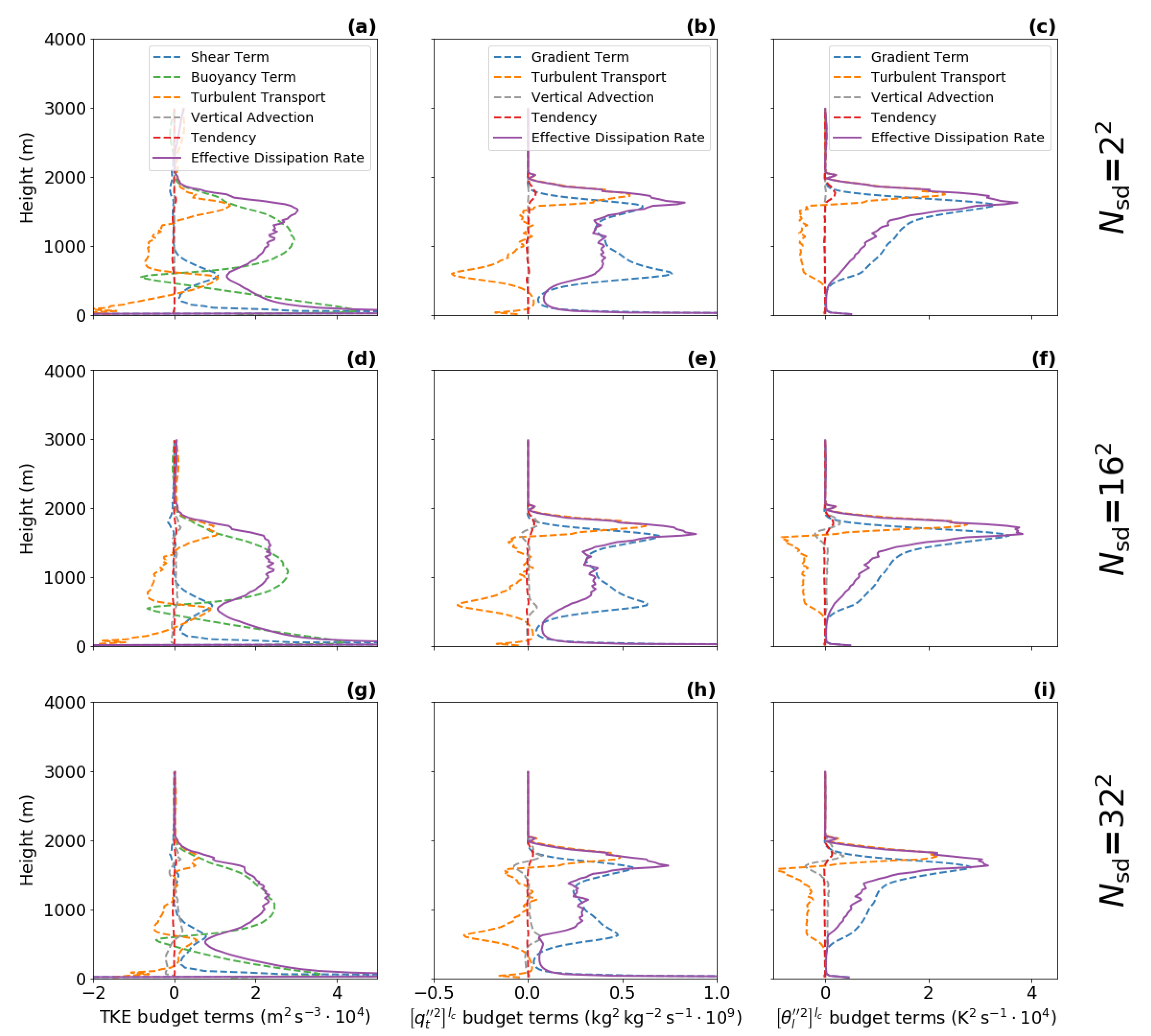
The new scale-aware turbulence length scales are computed from the effective dissipation rates, which are obtained from the variance budgets (see [3] and Section 2.3 for more details). To visualize the accuracy of the effective dissipation rates diagnostics, the individual terms of the three budgets are presented in Figure 1 for the BOMEX case.
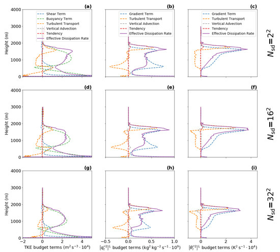
It can be seen that the grid spacing, vertical resolution, and the domain size of the LES are sufficient to obtain smooth profiles of the individual terms for all sub-domain sizes (only the results for the second largest, second smallest, and the smallest sub-domain sizes are shown). Such smooth profiles are necessary for further computation of the effective dissipation rates (violet lines). Similar results are found for all five idealized cases (not showed here). When comparing the diagnostics for different sub-domain sizes, the magnitude of the source terms (buoyancy term—green, gradient terms—blue), the turbulent transport terms (orange) is in general found to be smaller for the smaller sub-domain sizes.
The vertical advection terms (gray) should be equal to zero because horizontal homogeneity is assumed for all sub-domains. However, the vertical advection terms deviate from zero for the smallest sub-domains (). This implies that the condition of horizontal homogeneity is not fulfilled at this scale and thus the length scale diagnostics for the smallest sub-domain size is less accurate. Therefore, only results for larger sub-domains are used in the evaluation. The accuracy of the method for the smallest sub-domain size can be increased by including horizontal terms (i.e., the buoyancy, shear/gradient, and turbulence transport terms) in the respective budgets.
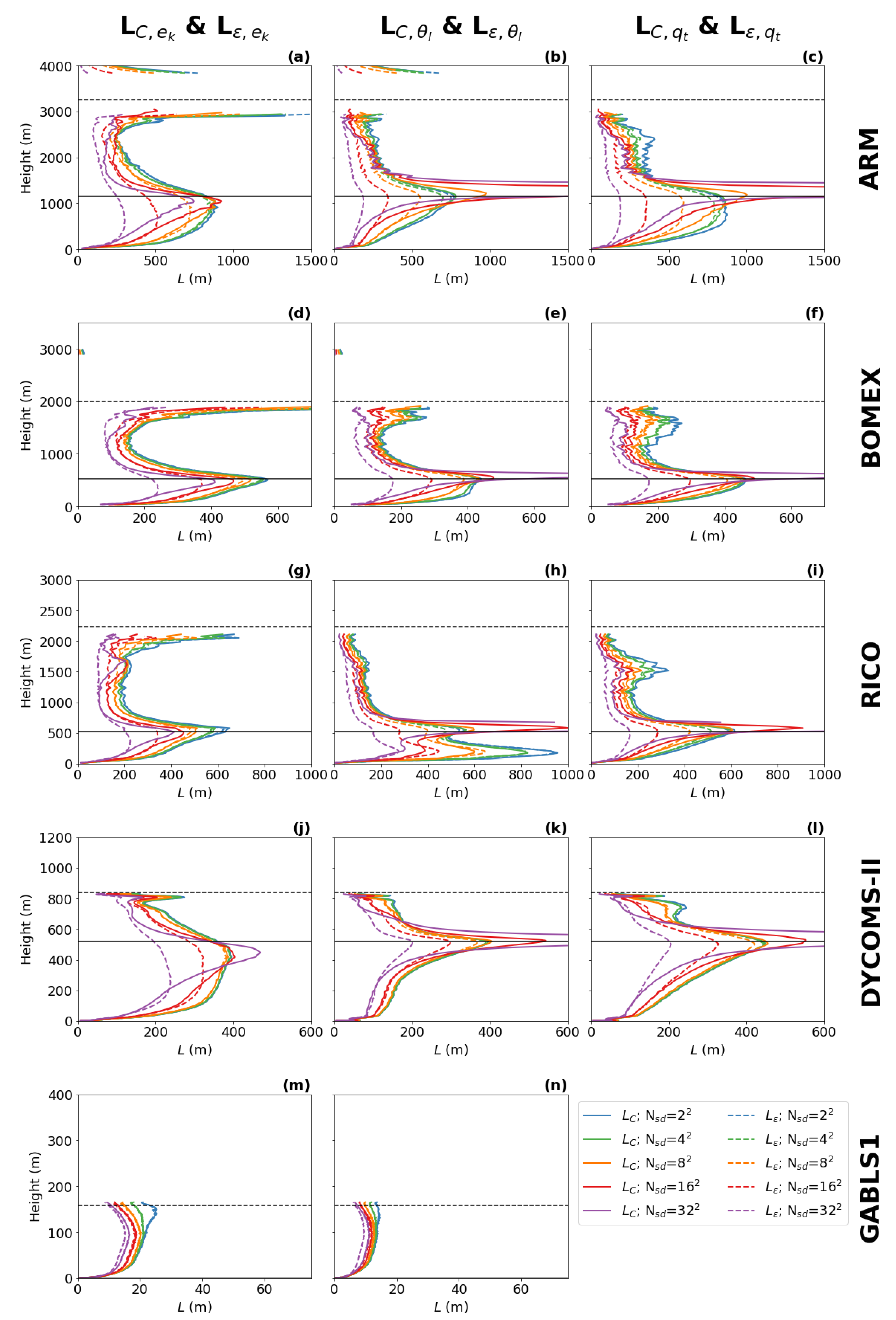
The turbulence length scale diagnostics resulting from the budgets can be seen in Figure 2 for all cases. As expected, all length scales have a similarly shaped profile. Near the surface, the length scale is proportional to the distance from the surface according to the von Karman theory. At higher levels, the length scale continues to grow, but the growth rate decreases until the length scale reaches a maximum in the ABL. The location and the intensity of this peak depend on the ABL regime, the resolution, and the type of diagnostic (see below). Above the peak, the turbulence length scale decreases towards the top of the ABL, where it reaches either a positive value or it converges to zero. The and diagnostics tend to show a secondary length scale peak near the top of the ABL in the convective cases (ARM, BOMEX, RICO) [3]. Such an increase in the turbulence length scale would imply an increase in the representation of the top entrainment. However, for the , , , and diagnostics, the secondary peak is either significantly smaller (ARM, BOMEX, RICO) or non-existent ( and for RICO). This suggests that the amplitude of the secondary peak in the and diagnostics is over-estimated due to the lower accuracy of the method caused by the presence of gravity waves near the top of the ABL [3].
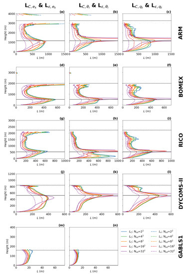
Figure 2.
The scale dependence of the turbulence length scale diagnostics based on the TKE budget (1st column; a,d,g,j,m), the variance budget (2nd column; b,e,h,k,n), and the variance budget (3rd column; c,f,i,l) for the five boundary layer cases (rows). The different sub-domain sizes are represented by different colors of lines, where the full lines are our new diagnostics () and dashed lines are the classical diagnostics (). indicates the number of sub-domains. and are not plotted for the dry GABLS1 case. The budgets are plotted for the ARM case after 10 h of integration, for the BOMEX and the RICO case after 7 h of integration and for the DYCOMS-II case and the GABLS1 case after 3 h of integration. The horizontal black dashed lines indicate the ABL height, and the horizontal black solid lines indicate the cloud base height.
In the cloudy cases, the location of the ABL peak correlates with the height of the cloud base. In the dry GABLS1 case, the peak is significantly weaker and is located roughly in the middle of the ABL. This means that the presence of clouds and related processes significantly affects the shape and the amplitude of the turbulence length scale profile.
At lower resolutions (larger sub-domains), the six different diagnostics are in general closer to each other for all cases. At higher resolutions (smaller sub-domain sizes), which enter the gray zone of turbulence (starting roughly with sub-domains), the differences between the classical (, and ) and new diagnostics (, , ) become more apparent. While the classically diagnosed turbulence length scales monotonously decrease with the sub-domain size due to their clear dependence on the TKE and the scalar variances, the changes in the new diagnostics are height-dependent because of their additional dependence on the effective dissipation rates [3]. Basically, the newly diagnosed length scales decrease more slowly or even increase in the region of the ABL peak and decrease faster in the remaining regions with increasing resolution. Such changes make the shape of the vertical profile of the turbulence length scales resolution-dependent, where the ABL peak is more pronounced at higher resolutions.
Similarly, there are also bigger differences visible between the diagnostic based on TKE (, ) and diagnostics based on scalar variances (, , , ) at higher resolutions. The ABL peak is sharper in the scalar variances diagnostics than in the TKE diagnostic. The scalar variances diagnostics are relatively close to each other with the exception of the RICO case, where the and have an additional strong peak in the sub-cloud layer. Differences between the TKE diagnostics and the scalar variance diagnostics in the ABL peak could be attributed to the accuracy of the diagnostic method, because the effective dissipation rates for scalar variances have relatively small values in the sub-cloud layer for higher resolutions (particularly for potential temperature variance). However, despite the potential accuracy issues, which is most evident in the highest resolution, the increase in the ABL peak for the scalar variances in the sub-cloud layer appears consistently in all cloudy cases. The differences between and , could indicate that the dissipation rates for scalars are not entirely proportional to the dissipation rates of TKE in the gray zone of turbulence as is usually assumed at lower resolutions (see, e.g., [7,14,31]), and that their dependence could be height- or regime-dependent.
3.2. Temporal Evolution of the Turbulence Length Scale Diagnostics
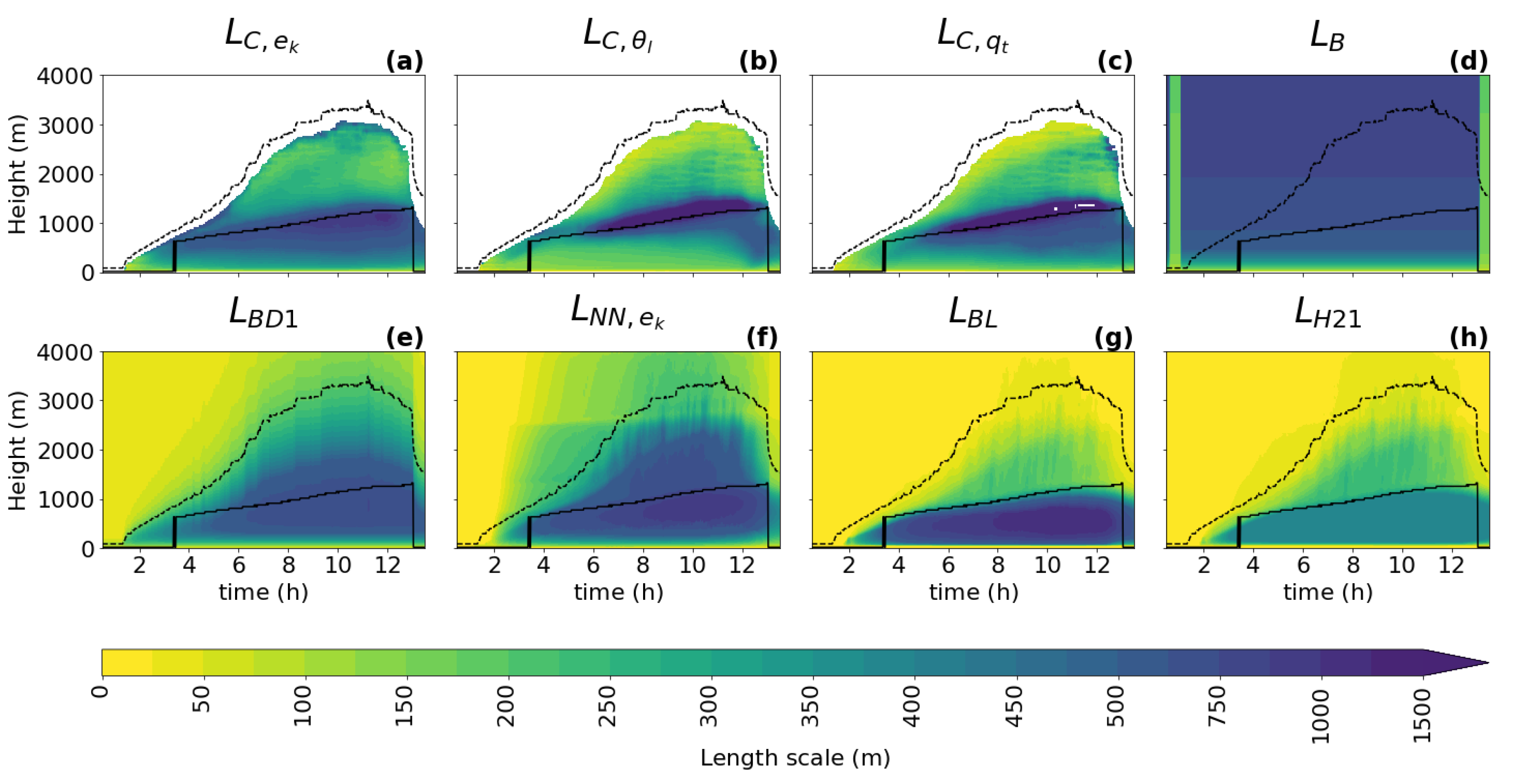
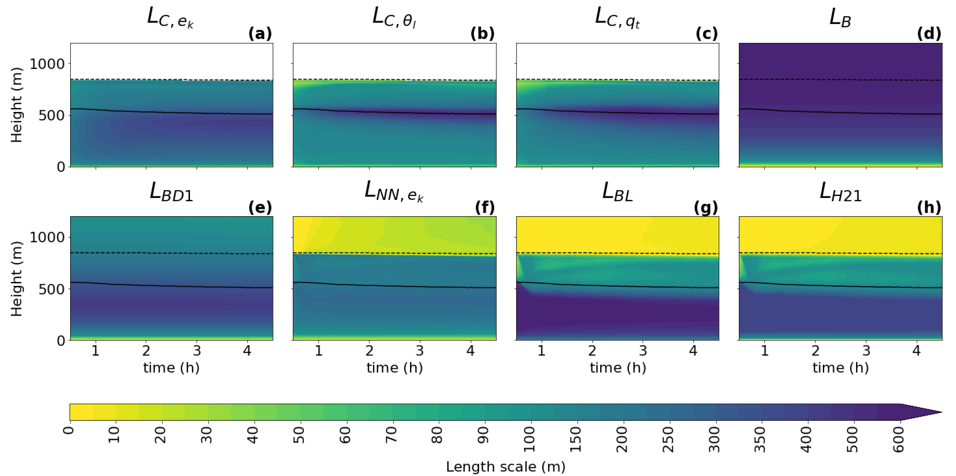
For a better understanding of the behavior of the turbulence length scale, we present the temporal evolution of its diagnostics in Figure 3a–c, Figure 4a–c, Figure 5a–c, Figure 6a–c and Figure 7a–c. Due to potential accuracy issues with the smallest sub-domain sizes (highest resolution), discussed in Section 3.1, the temporal evolution is analyzed for the second smallest sub-domain size.

Figure 3.
The temporal evolution of the turbulence length scale diagnostics: (a), (b), and (c); and the turbulence length scale formulations: (d), (e), (f), (g), and (h); for the ARM case. The length scales are computed for the second smallest sub-domain size (). The evolution of the cloud base height and the boundary layer height are represented by the black solid and dashed lines, respectively.
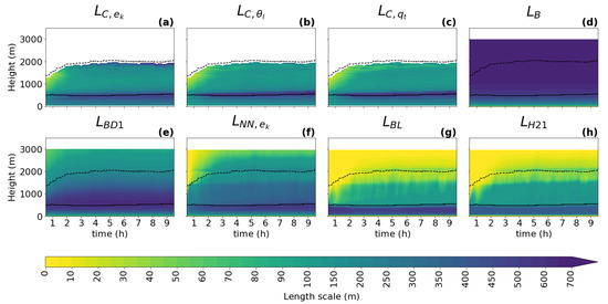
Figure 4.
Same content as Figure 3, but for the BOMEX case.

Figure 5.
Same content as Figure 3, but for the RICO case.
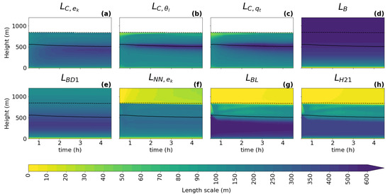
Figure 6.
Same content as Figure 3, but for the DYCOMS-II case.
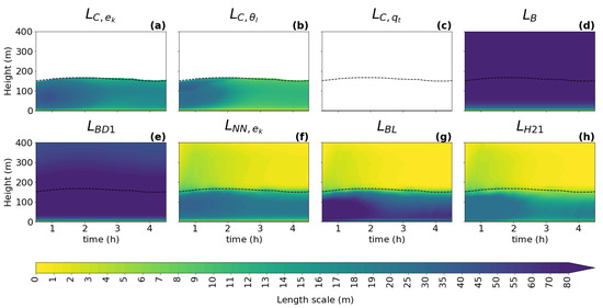
Figure 7.
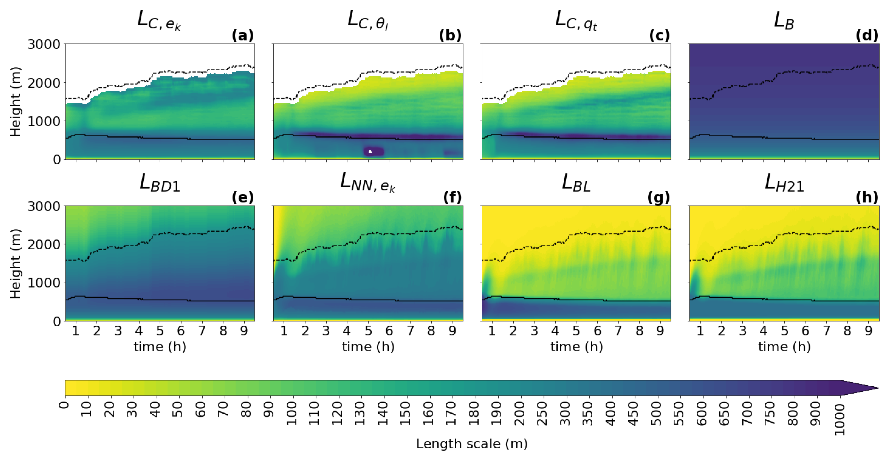
Same content as Figure 3, but for the GABLS1 case. is not plotted for the dry GABLS1 case.
For all cases, all diagnostics show a similar shape of the vertical profile for the turbulence length scale as described in Section 3.1: a linear increase with height near the surface; a peak in the ABL near the cloud base when clouds are present; and a decrease towards the ABL top, where zero or a positive asymptotic value is reached. As expected, it can be seen that the shapes of the profile follow the changes in the ABL height (dashed black line) and the cloud base height (full black line), which implies that these two heights should play an important role in the parameterization of the turbulence length scale. An exception to the dependence on the ABL height is visible in the initial phase of the GABLS1 case, where the amplitude of the ABL peak changes without any correlation to the ABL height (no clouds are present).
When comparing the three types of diagnostics (TKE, variance, and variance diagnostics), the results are consistent with findings in Section 3.1 for this (second smallest) sub-domain size, namely that the scalar variance diagnostics tend to have a more pronounced peak (sharper gradients of shading) in the ABL than the TKE diagnostic during the whole integration interval. Furthermore, a stronger secondary peak near the ABL top is present only in the TKE-based diagnostic.
3.3. Evaluation of the Algebraic Turbulence Length Scale Formulations
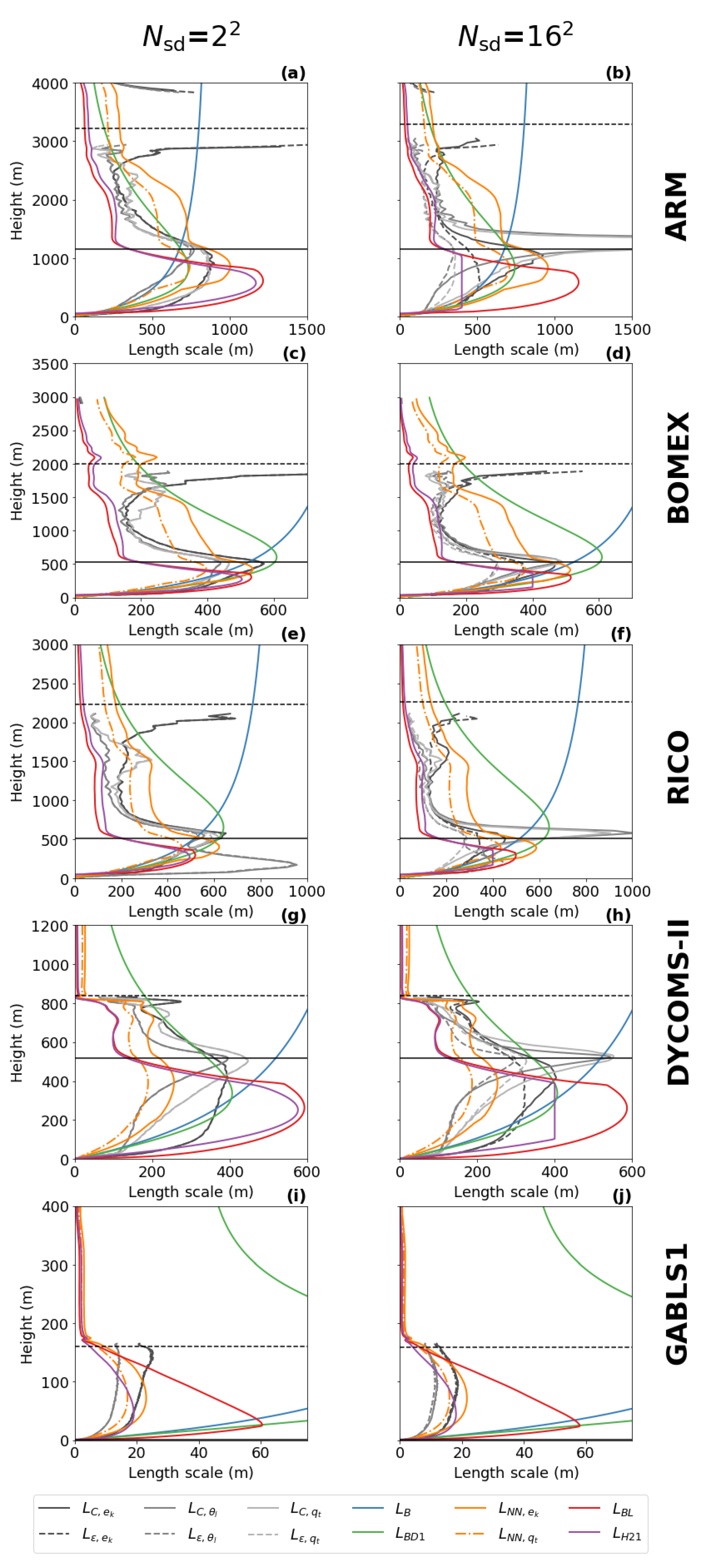
The selected algebraic formulations (see Section 2.2) computed from the coarse-grained LES data (see Section 2.3) are compared to the turbulence length scale diagnostics in Figure 8 for all cases.
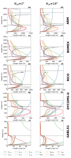
Figure 8.
Comparison of the turbulence length scale diagnostics (, , , , , and ) and the turbulence length scale formulations (, , , , , and ). Vertical profiles are plotted for the ARM case after 10 h of integration, for the BOMEX and the RICO case after 7 h of integration, and for the DYCOMS-II case and the GABLS1 case after 3 h of integration. and are not plotted for the dry GABLS1 case. The length scales are computed for the second-largest sub-domain size (1st column; a,c,e,g,i) and the second-smallest sub-domain size (2nd column; b,d,f,h,j). indicates the number of sub-domains.
All formulations exhibit an almost linear growth of the turbulence length scale near the surface as an extension of the von Karman theory, which is valid in the surface layer. A slight over-estimation compared to the diagnostics can be seen in the and formulations, which is caused by the influence of the upward length scale component, or , that can be larger than the distance from the surface. The linear behavior near the surface layer does not significantly change with the resolution.
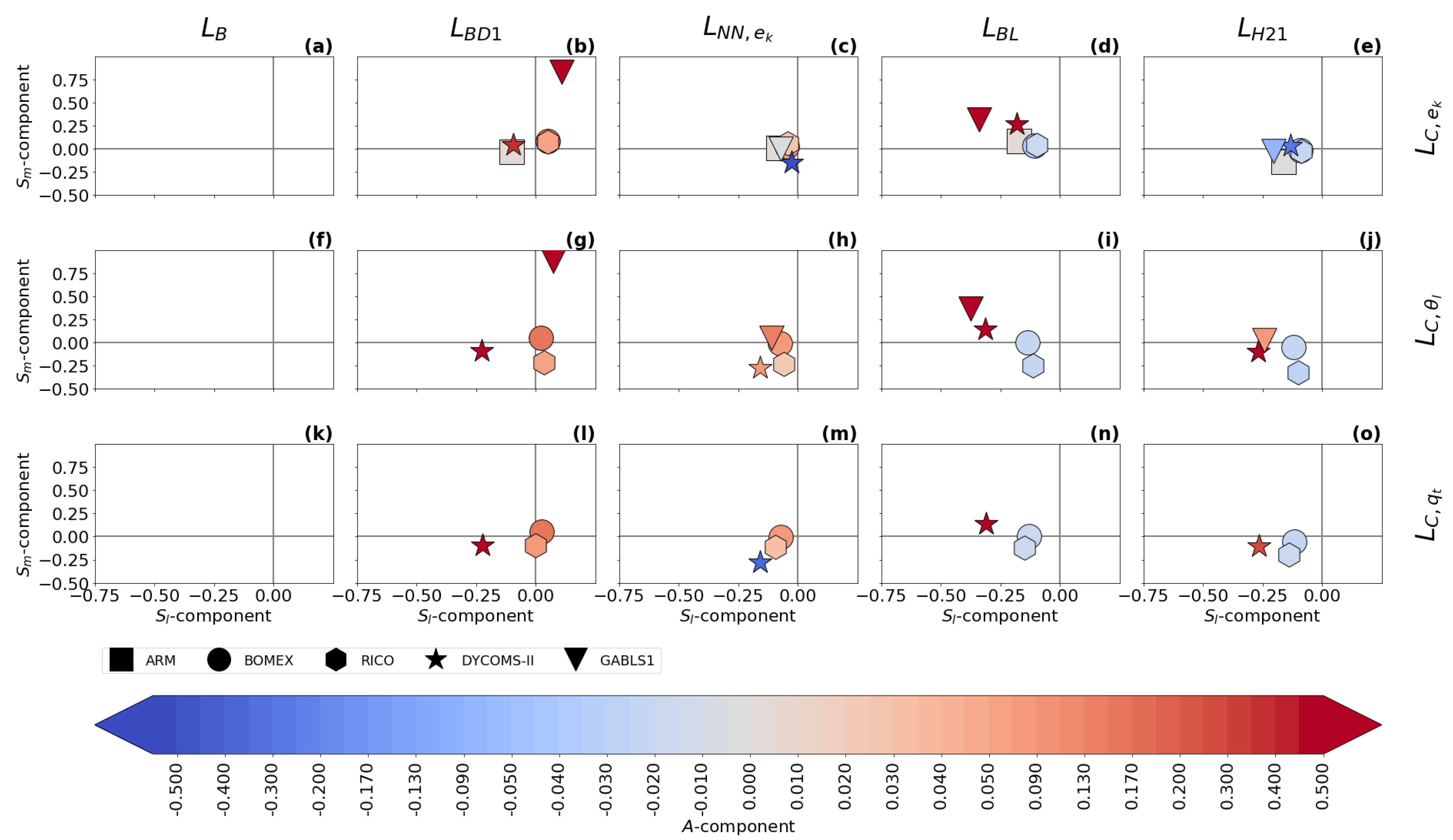
There are differences in the location and amplitude of the ABL peak between the length scale formulations. In order to achieve a more objective assessment of these characteristics, the time-averaged three-component plots (see Section 2.4) for two resolutions are presented in Figure 9 and Figure 10.

Figure 9.
The differences in the time averaged normalized magnitude, , and height/location, , of the ABL peak (see Equations (41) and (42)) between the turbulence length scale formulations: , , , , , and (columns); and the turbulence length scale diagnostics (rows; : (a–e), : (f–j), : (k–o)). The symbols represent the evaluation for each of the boundary layer cases, while the colors represent the time-averaged amplitude component, A (see Equation (39)). The scores are calculated for the second largest sub-domain size ().
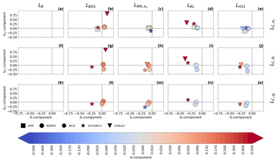
Figure 10.
Same content as Figure 9 but for the second smallest sub-domain size ().
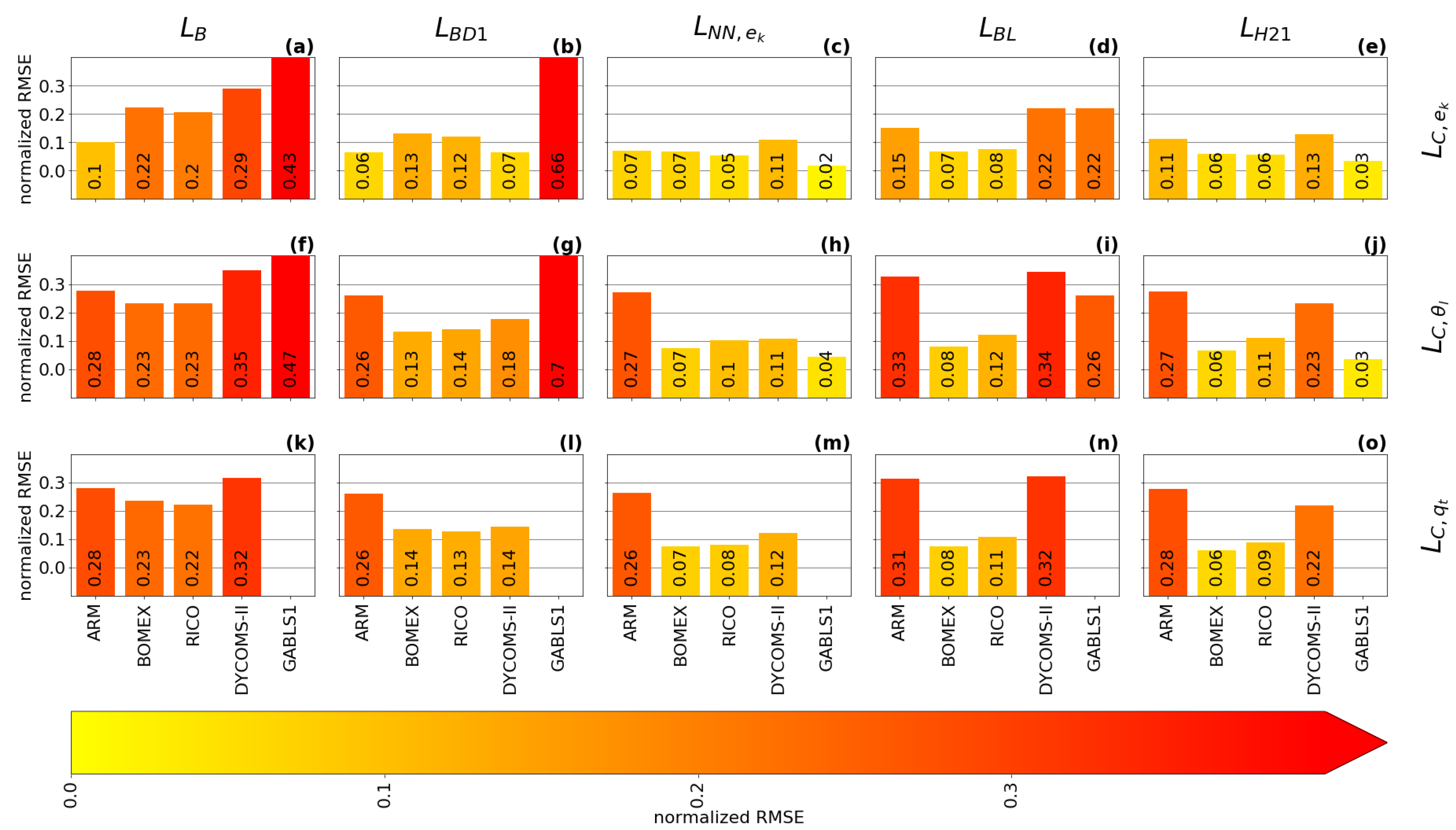
does not have an ABL peak, which significantly decreases its accuracy, as can be seen in the local normalized RMSE scores (see Equation (38)) that are presented in Figure 11 and Figure 12 for two selected resolutions. Additionally, is the same for all cases and all resolutions, because it depends only on the height.
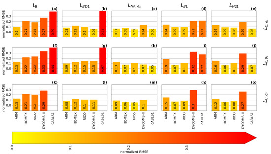
Figure 11.
The time-averaged normalized RMSE (see Equation (38)) of the turbulence length scale formulations: , , , , , and (columns); with respect to the three diagnostics (rows; : (a–e), : (f–j), : (k–o)). The normalized RMSE is calculated for the second-largest sub-domain size ().

Figure 12.
Same content as Figure 11, but for the second smallest sub-domain size ().
has a built-in ABL peak in its formulation, but its use is more suited for cloudy cases, where the estimation of the height and magnitude of the ABL peak is relatively accurate. strongly over-estimates the magnitude of the ABL peak in the GABLS1. While could be improved by calibration for the GABLS1 case, it would decrease its performance in the cloudy cases. Its overall performance across cases is thus limited. The shape of the profile is closer to the shape of the profile (the less pronounced ABL peak) than the profiles for scalar diagnostics. Therefore, its ABL peak estimation fits the TKE diagnostic better.
Both and significantly over-estimate the magnitude of the length scale in the GABLS1 case, which can be seen not only in the non-local overall mixing A-component (red color), but also in the local RMSE scores. The also over-mixes in the cloudy cases, except for the ARM case, but its local RMSE score is relatively good compared to other formulations. only scales with the ABL height; therefore, its overall performance decreases with increasing resolution.
, , and have A-component and RMSE scores similar to for the shallow convection cases (ARM, BOMEX and RICO). For these cases, their ABL peak magnitude closely matches the diagnosed magnitudes. However, their ABL peak is mostly placed below the diagnosed heights.
For the stratocumulus DYCOMS-II case, under-estimates the ABL peak magnitude, and and over-estimate the ABL peak magnitude and under-estimate the ABL peak height. In the GABLS1 case, over-estimates the amplitude and under-estimates the location of the ABL peak. shows a better ability in this respect. also shows a good ability due to its explicit dependence on the vertical wind shear (see Equations (35) and (36)). The differences in the ABL peak for DYCOMS-II and GABLS1 cases are also mirrored in the differences in the A-component and the RMSE scores.
Because , , and scale not only with the ABL height, but also with the TKE and stratification, their case-awareness is better than for and . Their resolution awareness is also improved due to this dependence. However, only shows significant adjustment to resolution due to its cut-off formulation (see Equation (32)). Therefore, out-performs at higher resolutions, particularly for the DYCOMS-II case, as can be seen in all scores. and are very close to each other at lower resolutions for the cloudy cases. shows better performance for higher resolutions. This is probably caused by the choice of that particular calibration rather than by the scale-awareness of , since changes relatively slowly with resolution.
When all aspects of the evaluation are taken in to account, shows the best performance among the selected length scale formulations. This is due to its composite formulation that introduces dependence to the ABL height, the TKE, and the stratification. Due to these properties, adjusts to the specific flow regimes in the selected cases. also slightly adapts to the changes in the resolution. However, under-estimates the height of the ABL peak compared to the diagnostics. The scale-awareness of is rather weak and depends on the specific calibration of the constants. and have similar scores to for the cloudy cases, but these formulations place the ABL peak even lower than and also over-estimate the ABL peak magnitude and overall mixing for DYCOMS-II. For the GABLS1 case, is comparable with and clearly out-performs due to its dependence on the vertical wind shear. While is well suited for cloudy cases, it strongly over-estimates the turbulence length scale for the GABLS1 case. Additionally, lacks scale awareness since it only scales with the ABL height. Adjustment to other resolutions and flow regimes can thus be achieved only via recalibration. is the simplest formulation, and thus it is not surprising that it has the worst scores. In particular, it does not have a peak in the ABL, and does not scale with any characteristic of the ABL.
When looking at the temporal evolution of the turbulence length scale formulations (Figure 3, Figure 4, Figure 5, Figure 6 and Figure 7), the above overall evaluation can be confirmed for all formulations. , , , and change according to the changes in the ABL height. does not have this dependence. In addition, the TKE-dependent formulations (, , ) are noisier than in the shallow convection cases, which could deteriorate their performance when used as an an active component of a numerical model.
4. Summary, Discussion, and Future Work
We have evaluated selected algebraic turbulence length scale formulations with budget-based turbulence length scale diagnostics that account for the cross-scale transfer of variances [3]. The diagnostics were computed using a coarse-graining method on high resolution LES data for selected idealized ABL cases: ARM (a continental cumulus case), BOMEX (a trade-wind cumulus case), RICO (a precipitating shallow cumulus case), DYCOMS-II (a stratocumulus case with drizzle), and GABLS1 (a weakly stable boundary layer case).
All vertical profiles of the length-scale diagnostics have a typical shape. Near the surface, the length scale is proportional to the distance from surface according to the von Karman theory. At higher levels, the length-scale growth rate decreases until it reaches a maximum in the ABL, whose location and intensity depend on the ABL regime, the resolution, and the type of diagnostic. Above the peak, the turbulence length scale decreases until it reaches an asymptotic value (positive or zero) at the top of the ABL.
In the cloudy cases, the location of the ABL peak correlates with the height of the cloud base. In the dry GABLS1 case, the peak is significantly weaker and is located roughly in the middle of the ABL. The new scale-aware diagnostics change with resolution (sub-domain size), but contrary to the changes in the classical turbulence length scale diagnostics, the resolution changes in the new diagnostics are height-dependent.
Compared to our previous study [3], we used not only the diagnostic based on the TKE budget, but also the diagnostics based on the budgets of the liquid-water potential temperature variance and the total specific-water-content variance. This extension helps to mitigate the accuracy problems of the TKE-based diagnostic in the presence of gravity waves in the convective cases near the top of the ABL, where the TKE diagnostic tends to show a secondary peak. Indeed, the scalar variance diagnostics indicate that the TKE diagnostic probably over-estimates the magnitude of this secondary peak in the ABL. In addition, we can observe that the ABL peak is sharper in the scalar variance diagnostics than in the TKE diagnostic. This could indicate that the dissipation rates for scalars are not entirely proportional to the dissipation rates of TKE in the gray zone of turbulence, as is usually assumed at lower resolutions, and that their dependence could be height- or regime-dependent.
We have used the local normalized RMSE (see Equation (38)) and the non-local three-component technique tailored specifically for the turbulence length scale profiles (see Section 2.4) for the evaluation of the turbulence length scale formulations.
Overall, shows the best performance among the selected length scale formulations. This is due to its multi-component composition and its dependence on the ABL height, the TKE, and the stratification. Thanks to these properties, adjusts to the specific flow regimes in the selected cases and also slightly adapts to the changes in the resolution. However, under-estimates the ABL peak location, and its scale-awareness could be stronger. and have similar scores to for the cloudy cases but are less accurate in the estimation of the ABL peak location and magnitude, particularly for the DYCOMS-II case. For the GABLS1 case, is comparable with and clearly out-performs due to its dependence on the vertical wind shear. is well suited for cloudy cases, but it strongly over-estimates the turbulence length scale for the GABLS1 case. Additionally, only scales with the ABL height, and thus it has almost no scale awareness. is the simplest formulation, and thus it is not surprising that it has the worst scores. In particular, it lacks the peak in the ABL and does not scale with any characteristic of the ABL.
When looking at the temporal evolution of the turbulence length scale formulations, , , , and adequately change according to the changes in the ABL height. In addition, the TKE-dependent formulations (, , ) are noisier than in the shallow convection cases, which could deteriorate their performance when used as an an active component of a numerical model.
It is clear from the evaluation that a proper scaling with the ABL height, TKE, stratification, and the vertical wind shear can improve the performance of the formulations. Such a scaling behavior makes the formulations more universal in terms of the ABL flow regime. To further improve this behavior, additional scaling variables could be introduced. In particular, all evaluated formulations have difficulties in the determination of the height of the ABL peak. As we have seen in the diagnostics, the ABL peak is usually placed just under the cloud base height. However, none of the formulations have an explicit dependence on the cloud base height, and thus the introduction of such a feature could be beneficial for future turbulence length scale formulations. We plan to investigate the scaling potential of the cloud base height in our future work.
The scale awareness in most of the evaluated formulations is relatively poor. The TKE’s dependence on the resolution and the stratification introduces a degree of scale awareness to , , , but it is not sufficient. Only shows a stronger scale awareness thanks to its cut-off formulation in the gray zone. However, in contrast to the turbulence length scale diagnostics, this dependence on resolution does not change with height. To improve the representation of turbulence in the gray zone of turbulence, we would recommend a turbulence length scale formulation that has a scale dependence that changes with height. We plan to propose such a formulation in our future work.
Better performance of the evaluated formulations can be achieved via recalibration of constants. This option can be used when changing the resolution of the model. Still, such a recalibration is rather time-consuming and does not support seamless changes in model resolution. Furthermore, a recalibration cannot be used to mitigate the lack of flow-regime dependence.
Based on our evaluation, we recommend using the , or formulation in TKE turbulence schemes. Nevertheless, we would like to point out that the turbulence length scale formulation is only a part of a turbulence scheme, and thus the overall performance of the scheme can decrease if the turbulence length scale formulation is changed. This is because the scheme was previously calibrated with a different length scale formulation. Hence, an introduction of a new turbulence length scale formulation requires recalibration of the whole scheme, and/or recalibration of other physical parameterizations of the model.
Author Contributions
Conceptualization, I.B.Ď.; methodology, I.B.Ď.; software, S.R., I.B.Ď. and A.T.J.; validation, S.R. and I.B.Ď.; formal analysis, S.R., I.B.Ď. and J.S.; investigation, S.R., I.B.Ď. and J.S.; resources, I.B.Ď. and J.S.; data curation, I.B.Ď.; writing—original draft preparation, S.R. and I.B.Ď.; writing—review and editing, S.R., I.B.Ď., J.S. and A.T.J.; visualization, S.R. and I.B.Ď.; supervision, I.B.Ď.; project administration, I.B.Ď.; funding acquisition, I.B.Ď. and J.S. All authors have read and agreed to the published version of the manuscript.
Funding
This research was funded by the Deutsche Forschungsgemenschaft (DFG) grant number 454477837 (GZ: BA 6804/2-1) and by the Hans Ertel Centre for Weather Research of DWD (3rd phase, The Atmospheric Boundary Layer in Numerical Weather Prediction) grant number 4818DWDP4. Furthermore, funded by the Deutsche Forschungsgemeinschaft (DFG, German Research Foundation)—TRR 301—Project-ID 428312742.
Institutional Review Board Statement
Not applicable.
Informed Consent Statement
Not applicable.
Data Availability Statement
The data for this study were generated with the LES model MicroHH and are openly available in Zenodo at https://zenodo.org/record/822842 [32] (accessed on 26 February 2022). The configuration files, outputs, and visualization scripts for the LES are openly available in Zenodo at: https://doi.org/10.5281/zenodo.6372434 [33] (accessed on 26 February 2022).
Acknowledgments
The authors would like to note that this research was made possible using the resources of the Deutsches Kimarechenzentrum (DKRZ) granted by its Scientific Steering Committee (WLA) under project ID bb1096.
Conflicts of Interest
The authors declare no conflict of interest.
Abbreviations
The following abbreviations are used in this manuscript:
| ABL | Atmospheric Boundary Layer |
| ARM | Atmospheric Radiation Measurement |
| BOMEX | Barbados Oceanographic and Meteorological Experiment |
| DYCOMS-II | the second Dynamics and Chemistry of Marine Stratocumulus |
| GABLS1 | GEWEX Atmospheric Boundary Layer Study |
| GEWEX | Global Energy and WAter Cycle Experiment |
| GCM | Global Circulation Model |
| LES | Large-Eddy Simulation |
| NWP | Numerical Weather Prediction |
| RICO | Rain in Shallow Cumulus Over the Ocean |
| RMSE | Root Mean Sqaure Error |
| TKE | Turbulence Kinetic Energy |
References
- Wyngaard, J.C. Turbulence in the Atmosphere; Cambridge University Press: Cambridge, UK, 2010. [Google Scholar] [CrossRef]
- Kitamura, Y. Estimating Dependence of the Turbulent Length Scales on Model Resolution Based on A Priori Analysis. J. Atmos. Sci. 2015, 72, 750–762. [Google Scholar] [CrossRef]
- Bašták Ďurán, I.; Schmidli, J.; Bhattacharya, R. A Budget-Based Turbulence Length Scale Diagnostic. Atmosphere 2020, 11, 425. [Google Scholar] [CrossRef] [Green Version]
- Wyngaard, J.C. Toward Numerical Modeling in the “Terra Incognita”. J. Atmos. Sci. 2004, 61, 1816–1826. [Google Scholar] [CrossRef]
- Honnert, R.; Masson, V.; Couvreux, F. A Diagnostic for Evaluating the Representation of Turbulence in Atmospheric Models at the Kilometric Scale. J. Atmos. Sci. 2011, 68, 3112–3131. [Google Scholar] [CrossRef]
- Honnert, R. Representation of the grey zone of turbulence in the atmospheric boundary layer. Adv. Sci. Res. 2016, 13, 63–67. [Google Scholar] [CrossRef]
- Bašták Ďurán, I.; Geleyn, J.F.; Váňa, F. A Compact Model for the Stability Dependency of TKE Production–Destruction–Conversion Terms Valid for the Whole Range of Richardson Numbers. J. Atmos. Sci. 2014, 71, 3004–3026. [Google Scholar] [CrossRef]
- Blackadar, A.K. The vertical distribution of wind and turbulent exchange in a neutral atmosphere. J. Geophys. Res. 1962, 67, 3095–3102. [Google Scholar] [CrossRef] [Green Version]
- Bašták Ďurán, I.; Geleyn, J.F.; Váňa, F.; Schmidli, J.; Brožková, R. A Turbulence Scheme with Two Prognostic Turbulence Energies. J. Atmos. Sci. 2018, 75, 3381–3402. [Google Scholar] [CrossRef]
- Bougeault, P.; Lacarrere, P. Parameterization of Orography-Induced Turbulence in a Mesobeta–Scale Model. Mon. Weather Rev. 1989, 117, 1872–1890. [Google Scholar] [CrossRef]
- Honnert, R.; Masson, V.; Lac, C.; Nagel, T. A Theoretical Analysis of Mixing Length for Atmospheric Models From Micro to Large Scales. Front. Earth Sci. 2021, 8, 537. [Google Scholar] [CrossRef]
- Nakanishi, M. Improvement of the Mellor–Yamada Turbulence Closure Model Based on Large-Eddy Simulation Data. Bound.-Layer Meteorol. 2001, 99, 349–378. [Google Scholar] [CrossRef]
- Nakanishi, M.; Niino, H. Development of an Improved Turbulence Closure Model for the Atmospheric Boundary Layer. J. Meteorol. Soc. Jpn. Ser. II 2009, 87, 895–912. [Google Scholar] [CrossRef] [Green Version]
- Cheng, Y.; Canuto, V.M.; Howard, A.M. An Improved Model for the Turbulent PBL. J. Atmos. Sci. 2002, 59, 1550–1565. [Google Scholar] [CrossRef] [Green Version]
- Lilly, D. The Representation of Small-Scale Turbulence in Numerical Simulation Experiments; Technical Report; National Center for Atmospheric Research: Boulder, CO, USA, 1966. [Google Scholar] [CrossRef]
- Stull, R.B. An Introduction to Boundary Layer Meteorology; Kluwer Academic Publishers: Amsterdam, The Netherlands, 1988. [Google Scholar]
- Redelsperger, J.L.; Mahé, F.; Carlotti, P. A Simple Furthermore, General Subgrid Model Suitable Both For Surface Layer Furthermore, Free-Stream Turbulence. Bound.-Layer Meteorol. 2001, 101, 375–408. [Google Scholar] [CrossRef]
- Cedilnik, J. Parallel Suites Documentation; Regional Cooperation for Limited Area modeling in Central Europe: Prague, Czech Republic, 2005. [Google Scholar]
- Mellor, G.L.; Yamada, T. A Hierarchy of Turbulence Closure Models for Planetary Boundary Layers. J. Atmos. Sci. 1974, 31, 1791–1806. [Google Scholar] [CrossRef] [Green Version]
- Bougeault, P.; André, J.C. On the Stability of the THIRD-Order Turbulence Closure for the Modeling of the Stratocumulus-Topped Boundary Layer. J. Atmos. Sci. 1986, 43, 1574–1581. [Google Scholar] [CrossRef] [Green Version]
- Rodier, Q.; Masson, V.; Couvreux, F.; Paci, A. Evaluation of a Buoyancy and Shear Based Mixing Length for a Turbulence Scheme. Front. Earth Sci. 2017, 5, 65. [Google Scholar] [CrossRef] [Green Version]
- Brown, A.R.; Cederwall, R.T.; Chlond, A.; Duynkerke, P.; Golaz, J.C.; Khairoutdinov, M.; Lewellen, D.C.; Lock, A.P.; MacVean, M.K.; Moeng, C.H.; et al. Large-eddy simulation of the diurnal cycle of shallow cumulus convection over land. Q. J. R. Meteorol. Soc. 2002, 128, 1075–1093. [Google Scholar] [CrossRef] [Green Version]
- Stevens, B.; Moeng, C.H.; Ackerman, A.S.; Bretherton, C.S.; Chlond, A.; de Roode, S.; Edwards, J.; Golaz, J.C.; Jiang, H.; Khairoutdinov, M.; et al. Evaluation of Large-Eddy Simulations via Observations of Nocturnal Marine Stratocumulus. Mon. Weather Rev. 2005, 133, 1443–1462. [Google Scholar] [CrossRef] [Green Version]
- Holtslag, B. Preface: GEWEX Atmospheric Boundary-layer Study (GABLS) on Stable Boundary Layers. Bound.-Layer Meteorol. 2006, 118, 243–246. [Google Scholar] [CrossRef]
- Beare, R.J.; Macvean, M.K.; Holtslag, A.A.M.; Cuxart, J.; Esau, I.; Golaz, J.C.; Jimenez, M.A.; Khairoutdinov, M.; Kosovic, B.; Lewellen, D.; et al. An Intercomparison of Large-Eddy Simulations of the Stable Boundary Layer. Bound.-Layer Meteorol. 2006, 118, 247–272. [Google Scholar] [CrossRef] [Green Version]
- Siebesma, A.P.; Bretherton, C.S.; Brown, A.; Chlond, A.; Cuxart, J.; Duynkerke, P.G.; Jiang, H.; Khairoutdinov, M.; Lewellen, D.; Moeng, C.H.; et al. A Large Eddy Simulation Intercomparison Study of Shallow Cumulus Convection. J. Atmos. Sci. 2003, 60, 1201–1219. [Google Scholar] [CrossRef]
- Rauber, R.M.; Stevens, B.; Ochs, H.T.; Knight, C.; Albrecht, B.A.; Blyth, A.M.; Fairall, C.W.; Jensen, J.B.; Lasher-Trapp, S.G.; Mayol-Bracero, O.L.; et al. Rain in Shallow Cumulus Over the Ocean: The RICO Campaign. Bull. Am. Meteorol. Soc. 2007, 88, 1912–1928. [Google Scholar] [CrossRef] [Green Version]
- van Heerwaarden, C.C.; van Stratum, B.J.H.; Heus, T.; Gibbs, J.A.; Fedorovich, E.; Mellado, J.P. MicroHH 1.0: A computational fluid dynamics code for direct numerical simulation and large-eddy simulation of atmospheric boundary layer flows. Geosci. Model Dev. 2017, 10, 3145–3165. [Google Scholar] [CrossRef] [Green Version]
- Baas, P.; de Roode, S.R.; Lenderink, G. The Scaling Behaviour of a Turbulent Kinetic Energy Closure Model for Stably Stratified Conditions. Bound.-Layer Meteorol. 2007, 127, 17–36. [Google Scholar] [CrossRef]
- Wernli, H.; Paulat, M.; Hagen, M.; Frei, C. SAL—A Novel Quality Measure for the Verification of Quantitative Precipitation Forecasts. Mon. Weather Rev. 2008, 136, 4470–4487. [Google Scholar] [CrossRef] [Green Version]
- Zilitinkevich, S.S.; Elperin, T.; Kleeorin, N.; Rogachevskii, I.; Esau, I. A Hierarchy of Energy- and Flux-Budget (EFB) Turbulence Closure Models for Stably-Stratified Geophysical Flows. Bound.-Layer Meteorol. 2012, 146, 341–373. [Google Scholar] [CrossRef] [Green Version]
- van Heerwaarden, C.C.; van Stratum, B.J.H.; thijsheus. microhh/microhh: 1.0.0. 2017. Available online: https://zenodo.org/record/822842 (accessed on 26 February 2022).
- Bašták Ďurán, I.; Reilly, S.; Anurose, T.J.; Schmidli, J. Data Accompanying the Paper Titled: An Evaluation of Algebraic Turbulence Length Scale Formulations. 2022. Available online: https://zenodo.org/record/6372434 (accessed on 26 February 2022).


Publisher’s Note: MDPI stays neutral with regard to jurisdictional claims in published maps and institutional affiliations. |
© 2022 by the authors. Licensee MDPI, Basel, Switzerland. This article is an open access article distributed under the terms and conditions of the Creative Commons Attribution (CC BY) license (https://creativecommons.org/licenses/by/4.0/).