Abstract
Granularity of the grid (both horizontally and vertically) is a key consideration when conducting localised Numerical Weather Prediction (NWP) modelling. Generally speaking, an NWP model with a finer grid can explicitly resolve more processes and require less parameterisation. However, a finer grid also requires more computation and it is not always clear that a finer grid will produce a more accurate forecast. In this study, we explore the sensitivity of rainfall prediction over Singapore to grid resolution. We use the Weather and Research Forecasting model (WRF) to forecast rainfall over Singapore and explore the performance of horizontal resolutions ranging from 1 km to 12 km. We test the performance on a set of dates from across the years 2020–2021 against both ground observations and radar-derived rain rates. When compared to ground observations, we show that, overall, the higher resolution produces the highest Critical Success Index (CSI) for rain rates in excess of 0.5 mm/h. When compared against radar-derived rain rates, the 1 km domain produces superior CSI values for all rain rates. The daily-average hourly Fractional Skill Score (FSS) was then calculated for some dates and showed agreement with the CSI results with the exception of a north-east monsoon day where, for heavier rain rates, the 3 km domain has superior FSS. We also investigate a particularly heavy rain event on 10 January 2021 and show that the 3 km grid has highest CSI for rain rates of 4 mm/h and 16 mm/h (based on both ground-based and radar-derived rain rates), however, the 1 km has superior FSS for this event.
1. Introduction
Methods for improving the prediction of rainfall is an ongoing area of research in the field of meteorology. Interest stems not only for academic reasons, but also due to the implication that accurate rainfall forecasts have the potential to save lives and avoid damage to infrastructure through better planning and awareness. For instance, [1] estimated that floods kill 12,700 people annually and some hard-hit countries such as China have faced damages of 1–3% of Gross National Product due to flooding [1]. In their latest report (AR6), the International Panel on Climate Change (IPCC) have confirmed that some areas of the globe have seen significant increases in precipitation since the beginning of the 20th century [2] and that the world may see a 15% increase in the intensity of both 1-in-10-year and 1-in-50-year extreme precipitation events under a 2 °C warmer climate [3]. Thus, the accurate prediction of such events requires the attention of meteorologists.
Methods for forecasting rainfall vary depending on the location and time horizon. For short time horizons (i.e., 0–6 h) and less chaotic locations, the methods of nowcasting have useful predictive power. Ref. [4] reviewed the use of Convolutional Neural Networks (CNNs) for nowcasting from radar images. Ref. [4] showed that for a heavy rain event in Braunsbach, Germany, the CNN is able to compare with more traditional techniques such as optical flow. Others have also tried blending radar and observations in a nowcasting method [5], while Singapore (the focus area of this study) [6] utilised GPS-estimates of precipitable water vapour to conduct very short (5 min ahead) prediction of rain events in 2014 and 2015.
However, for locations that experience rapidly evolving atmospheric processes, or for longer time horizons (i.e., beyond 4–6 h), physical models that can both spin-up and rain-out convective systems are necessary. Such models fall into the category of Numerical Weather Prediction (NWP) models. NWP models approximate the fluid and thermodynamic equations—often through discretisation of the governing equations and stepping forward in time through methods like Runge–Kutta. Other processes important for weather prediction, such as the transfer of radiation through the atmosphere and small-scale processes such as microphysics (phase changes within a cloud) require parameterisation in order for NWP models to be computationally efficient. How best to estimate the processes requiring parameterisation is an active area of research and models such as the Weather and Research Forecasting (WRF) model [7] have a vast array of options for each process that is parameterised.
Ref. [8] investigated over 100 possible choices of WRF model configuration, in addition to the performance of various spatial resolutions, for the forecast of precipitation over British Columbia, Canada. Over complex terrain, Ref. [8] found the Kain–Fritsch to be generally better than the Grell–Frietas cumulus scheme and that there was clear seasonal dependence in the best performing scheme combinations. In addition, the authors found better representation of the distribution of precipitation values from the higher resolution domains (3 km versus 27 km) but that the coarser resolutions had higher equitable threat scores (overall performance). On the contrary, Ref. [9] found greater skill in higher resolution, convection-permitting simulations over tropical east Africa. In Singapore, a collaboration between the United Kingdom’s Met Office and Meteorological Services Singapore, which gave rise to the SINGV model [10], also found better skill at higher resolution. Analysis of the performance of SINGV in Ref. [10] shows a clear improvement in rainfall forecast skill from the 1.5 km model when compared to the coarser 11 km grid.
The SINGV model represents a significant step forward for operational weather forecasting in Singapore, which is a challenging location to forecast. Located at roughly 1° N and 104° E, Singapore is an island state and maritime continent that experiences significant rainfall throughout the year. Following the shift in the meteorological equator, the prevailing winds deliver two monsoon seasons and two inter-monsoon/transition seasons. During the north-east monsoon (December–February), prevailing winds in addition to interactions with land–sea thermal contrasts can produce prolonged periods of rain. During the south-west monsoon (June–September), so-called Sumatran squalls are most common, which often bring heavy outbursts of rainfall in the early hours/pre-dawn. Inter-monsoon periods are characterised by generally light winds and diurnally forced afternoon storms. Ref. [11] also investigated the use of WRF for rainfall modelling in Singapore. The authors investigated several physical scheme combinations on 14 rain events from 2011. Ref. [11] found that even at 1 km resolution, the maximum intensity of rainfall from their output was much lower than the observations and that the cause could be due to low resolution geographical data leading to insufficient representation of land–sea processes.
In this paper, we explore the influence of spatial resolution on rainfall modelling over Singapore. As was mentioned previously, SINGV at 1.5 km showed improved forecast skill when compared to the control experiment at 11 km. Others have found similar results when it comes to increased skill in rainfall modelling with increased spatial resolution; the general idea being that higher spatial resolutions begin to resolve convection processes explicitly without the need for parameterisation. Refs. [9,12] both note the importance of running NWP models at the convection permitting scale. Meanwhile, Ref. [13] compared 1, 4, 8 and 16 km resolutions for flood forecasting in north-eastern Italy and found generally larger errors from the 16 km domain compared to the 1 km resolution. Similar results were also found by Ref. [14] in Peru showing that 0.75 km resolution WRF grid was able to better produce local processes and that the 18 km domain had the lowest skill.
We therefore wish to test the hypothesis that higher resolution WRF grids will also achieve greater skill when forecasting rainfall over Singapore. The rest of this paper is structured as follows: Section 2 describes the methods and observations, Section 3 presents the results for both the 15-day testing set and the heavy rain event, while Section 4 concludes the study and suggests future work arising from the results.
2. Experimental Methods
2.1. Observations
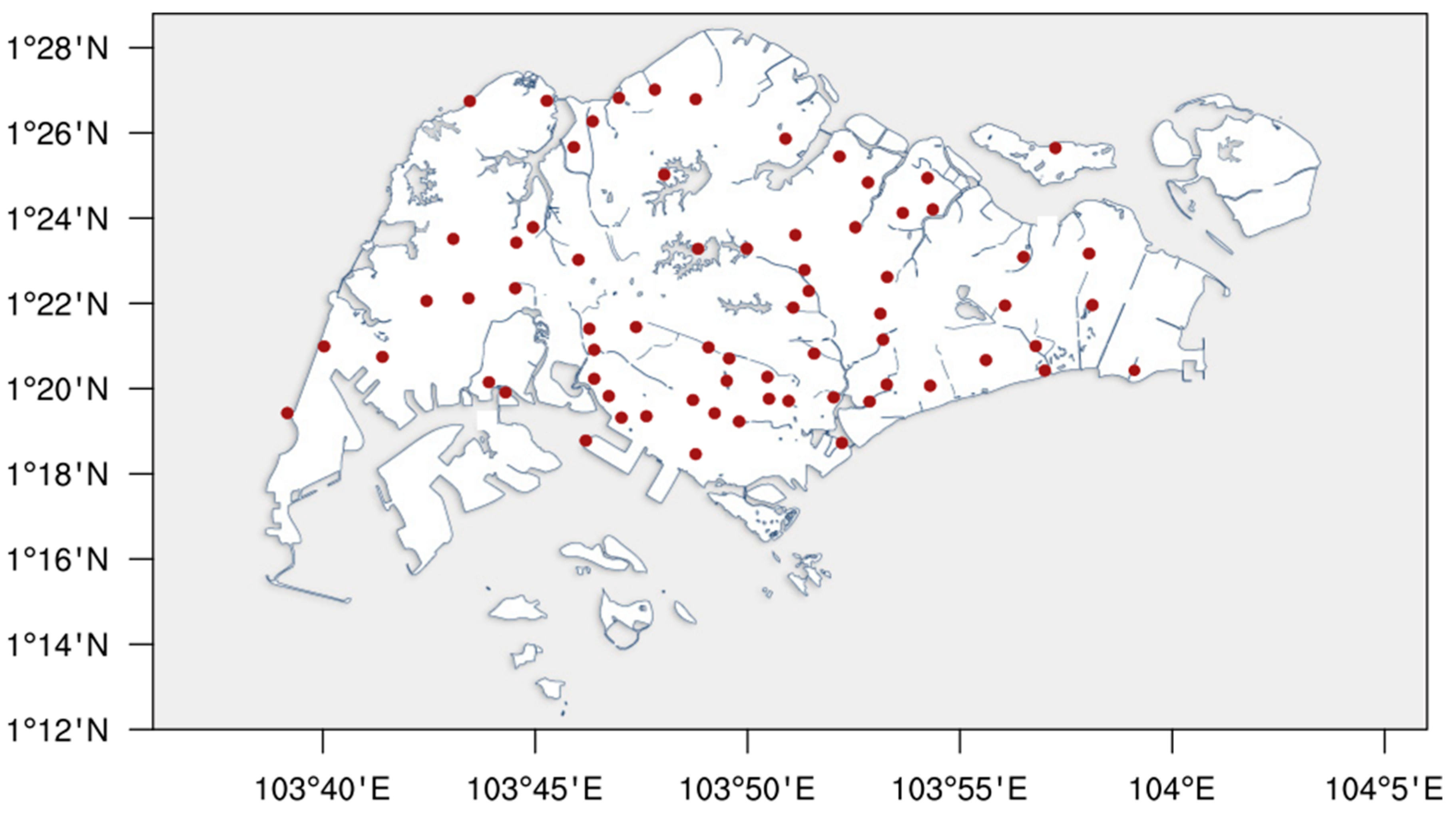
The study period examined covers dates from the years 2020–2021 for the general case and focuses on 10 January 2021 for the heavy rain event. Observations cover the entire island of Singapore courtesy of the National Environment Agency API (https://data.gov.sg/dataset/realtime-weather-readings, accessed on 6 April 2022). Figure 1 shows the location of the observation stations.
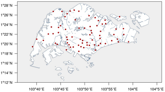
Figure 1.
Location of observation stations across Singapore. Background map adapted from National Environment Agency website.
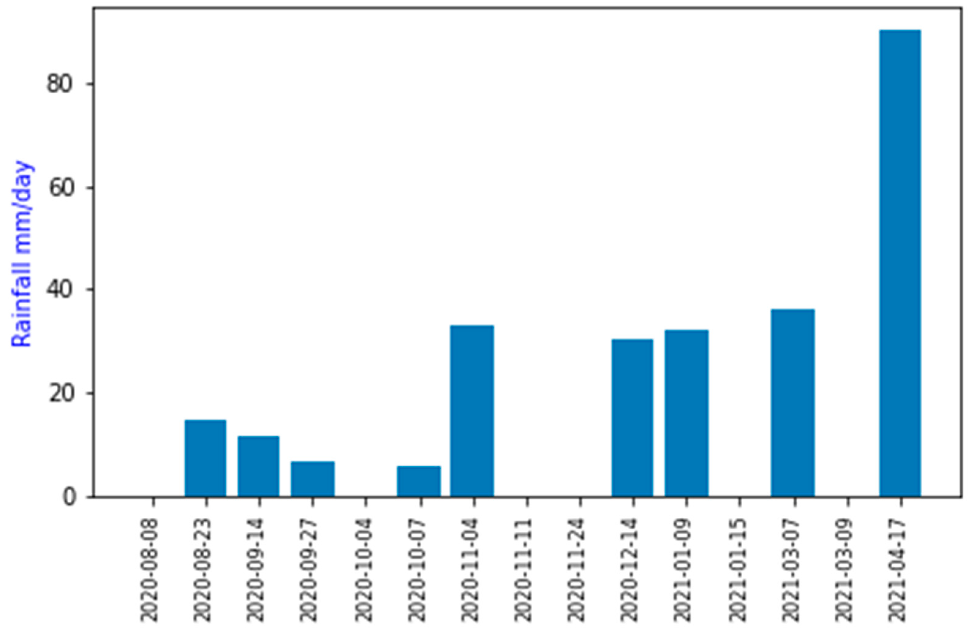
Rain at the hourly rate (mm/h) from August 2020 to April 2021 was analysed and 15 days from this period were selected for analysis. Selection of the days was conducted such that a mixture of no-rain, light-medium rain and medium-heavy rain days were included in the testing set. In addition, selection was done to maximise the representation across the seasons in Singapore: north-east monsoon (December–February), south-west monsoon (June–September) and inter-monsoon (October–November/March–May). The Singapore-wide average daily rainfall for the days selected are shown in Figure 2.

Figure 2.
Days used in the study to analyse rainfall forecast performance. Dates are listed in local time (SGT) for the midnight to midnight period and rainfall amounts are the average across Singapore.
2.2. Radar-Derived Rain Rates
In addition to the ground observations covering the Singapore island, radar-derived rain rates were included as a truth for comparison with the forecast experiments. The 240 km radar, which covers an extent beyond Singapore and is maintained by the National Environment Agency, was archived for the study period through downloading the images at a publicly available website (for instance, http://www.weather.gov.sg/files/rainarea/240km/dpsri_240km_2022040802300000dBR.dpsri.png, accessed on 6 April 2022) in real-time. The radar images were then transformed into rain rate estimates by converting pixel colour to rain rate intensity, utilising example charts that outline the colour table and rain rate levels. In addition, pixel location was estimated by creating a 1 km grid (the resolution of the radar) to the latitude and longitude extents of the background map. Verification of the method to extract rain rates utilising the ground observations for the dates in the study shows reasonable concordance (Table 1).

Table 1.
Comparison of radar-derived rain with ground observations for the dates in the study. See Section 2.4 for definition of the metrics.
2.3. Numerical Weather Prediction
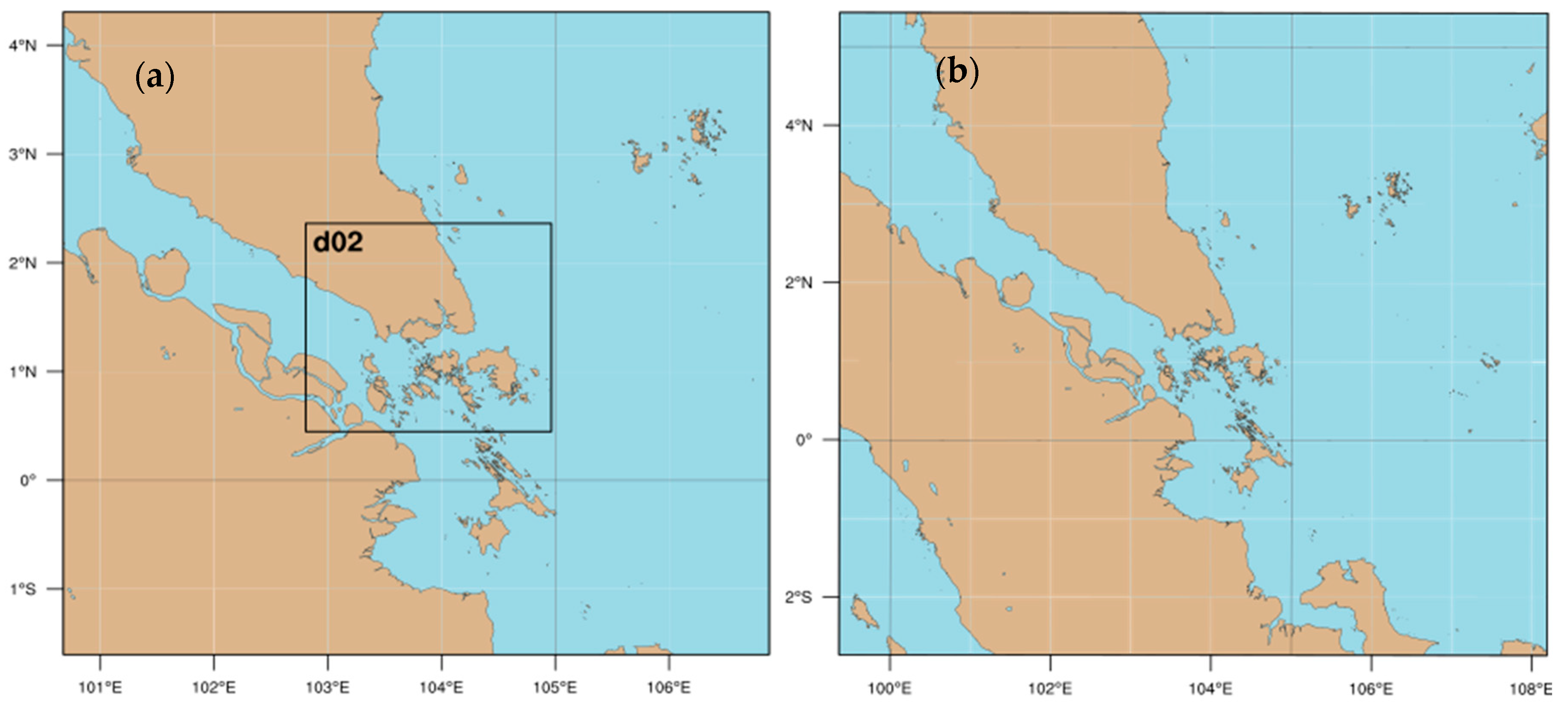
In this study, we utilised one of the most common and widely used NWP models—the Weather and Research Forecasting model (WRF). The WRF model is a fully compressible conservative-form nonhydrostatic model and is suitable for both operational and research purposes [7]. At the time of this writing, WRF is up to version 4, however, we utilised the WRF model version 3.9.1 for this paper. We utilised the WRF model in a limited-area setting and thus also required initial and boundary conditions to run the model. We utilised the 12UTC initial and boundary conditions from the High-Resolution (HRES) deterministic model operated by the European Centre for Medium Range Weather Forecasting (ECMWF) for all experiments. ECMWF model inputs were used at a 3-hour interval and with spatial resolution of 0.1°. Several domains were set-up to test the influence of the WRF spatial resolution on rainfall simulation over Singapore. Figure 3a outlines the 3 km (parent) and 1 km (daughter) domains and Figure 3b shows the 9 km and 12 km domains. For all domains, the simulations were run for 28 h. Hours 0–4 were not analysed as spin-up and rainfall accumulation from hours 4–5 until hours 27–28 were analysed, which also corresponds to the midnight to midnight period in local time.
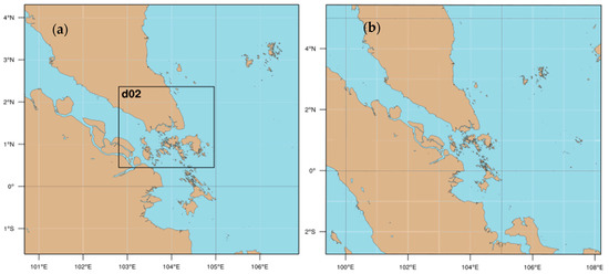
Figure 3.
WRF model domains. In (a), the 3 km parent domain (defined by the picture boundary) with the 1 km domain within (d02) and in (b), the domain extent for both the 9 km and 12 km experiments.
2.4. Measuring Forecast Performance
WRF total precipitation values were compared to the ground observations and radar-derived rain rates at hourly accumulation via four main measures: Hit-Rate (HR), False-Alarm Rate (FAR), Critical Success Index (CSI) and Fractions Skill Score (FSS). The first three measures utilise the contingency table, which is defined in Table 2 below:
Table 2.
Contingency table outlining the categories when the Forecast (F) and/or the Observed (O) rainfall are above and below a given threshold (T in mm/h).
From the contingency table, the HR, FAR and CSI are calculated, for a given threshold, as follows:
The HR describes the proportion of hits () in relation to the total hits and misses (), the FAR describes the proportion of false-alarms () to the total hits and false-alarms () and the CSI describes the proportion of hits () to the total hits, false-alarms and misses (). The above metrics were analysed at the hourly rain rate and for the 24 h period from each of the 15 dates outlined in Figure 2, as well as the 10 January 2021 heavy rain day. Forecast values of total precipitation were compared to the observed values for all stations across the Singapore island (Figure 1) and the WRF model grid points were selected based on the nearest grid point (distance to the observed point). Additionally, WRF model grids were re-gridded to match the grid of the Singapore 240 km radar and the above metrics were then also calculated across the grid. Various hourly rainfall thresholds were analysed to determine if model performance varied based on the rainfall intensity and these thresholds were: 0.0 mm/h, 0.5 mm/h, 1 mm/h, 2 mm/h, 4 mm/h, 8 mm/h, 16 mm/h, 32 mm/h and 64 mm/h.
Finally, the fourth measure of forecast performance is the FSS [15]. The FSS in this paper was calculated following the fast method outlined in Ref. [16]. The FSS analyses the fraction of an area covered by rain in the forecast and compares that fraction to the observed fraction of the same area. In this way, a forecast that has the rain location slightly wrong can still be considered skilful where it might otherwise have poor contingency table scores. It is also necessary for the observed and forecast values to have the same grid and for this study, we re-gridded the forecasts to match the observed grid. We then also limited the calculation of the size of the smallest domain (the 1 km domain shown in Figure 3). The FSS is calculated for various area sizes and rain rates and is represented mathematically by Equations (4) and (5).
where and represent the fraction of a given area/window containing rainfall in the forecast () or observation () and where the difference is squared and summed over neighbourhoods in the domain. The average of this sum is the FBS, which is utilised in the calculation of the FSS as follows:
The FSS is oriented such that a larger value indicates more skill and where 0 is no skill and 1 is a perfect forecast. In addition, the usefulness of the forecast can be estimated using the metric outlined in Ref. [17]. The can be calculated as follows:
where represents the fraction of the domain that contains rain.
2.5. Choosing WRF Configuration
WRF configuration options were selected based on previous work (not presented here). A process for optimising the physics options important to rainfall (cumulus parameterisation, microphysics, planetary boundary layer and surface schemes) similar to that outlined in Ref. [18] was conducted for the 3 km domain. These, plus other important options are outlined in Table 3. In this study, the coarser resolutions (9 km and 12 km) utilised the same set of physics as the 3 km, however, for the 1 km cumulus, parameterisation was turned off as it is assumed to be a fine enough resolution to begin explicitly resolving convective processes.
Table 3.
Selection of important physics options utilised in the current study.
3. Results
The following result sections outline the results of the various spatial resolutions on the testing set of 15 days, as well as the heavy rain day. Analysis is presented via the metrics outline in Section 2.4 as well as via spatial comparison with radar images. Comparison between observed point values and gridded forecast values was performed by utilising the nearest gridded value (spatial distance) for each observed point.
3.1. Performance on Testing Set Compared to Ground Observations
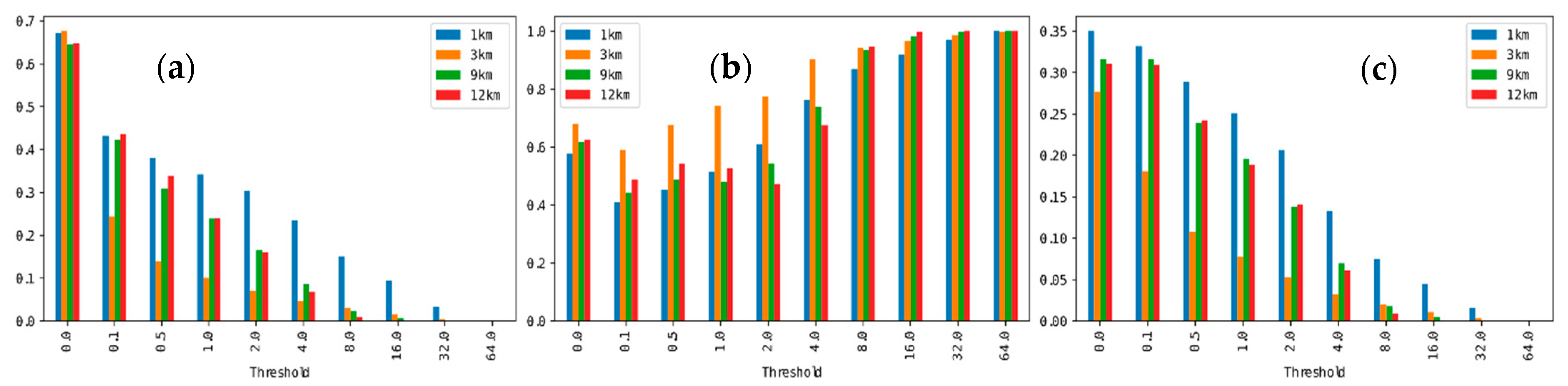
Overall performance on the 15-day testing set is outlined in Figure 4. What is clear from Figure 4 is that for rain rates at or above 1.0 mm/h, the 1 km domain is clearly superior—both in terms of hit-rate and CSI. The 12 km domain had superior CSI for 0.5 mm/h but evidently struggled to produce heavier rain rates with no hits or false-alarms from 4.0 mm/h and above.
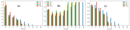
Figure 4.
Performance of various WRF spatial resolutions versus rainfall threshold. In (a), the HR, in (b), the FAR and in (c), the CSI for the 15-day testing set.
Looking more closely at some of the individual days, we can see this more clearly. Table 4, Table 5 and Table 6 show the HR, FAR and CSI for select rain rates and days. The three days represent a Sumatran squall (early hours of 4 November 2020), a north-east monsoon day (afternoon of 9 January 2021) and an afternoon squall (afternoon of 17 April 2021).
Table 4.
Metrics for 4 November 2020.
Table 5.
Metrics for 9 January 2021.
Table 6.
Metrics for 17 April 2021.
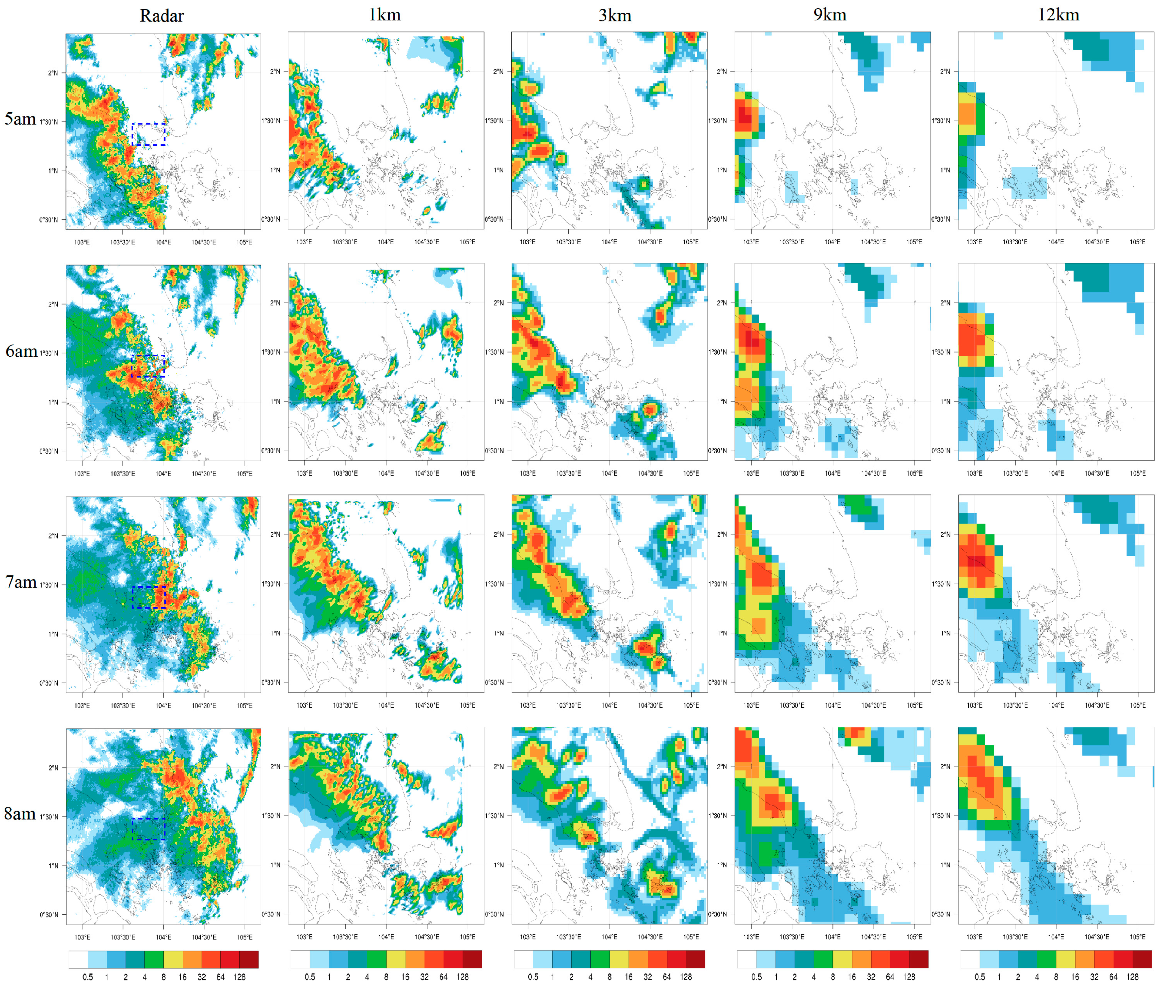
The 4 November 2020 event was characterised by a squall-line passing over Singapore from 5 am (Figure 5). For the small rain rates, the 1 km and 3 km domains have best performance while the heavier rain rates are dominated by the 1 km domain. When plotted against the radar, we can see in Figure 5 that all domains have slightly incorrect timing (late) but that the 1 km domain has the most accurate-looking features. As all model domains are driven by the same ECMWF conditions, it is hypothesised that the reason for the incorrect timing originates with issues in the global model conditions.
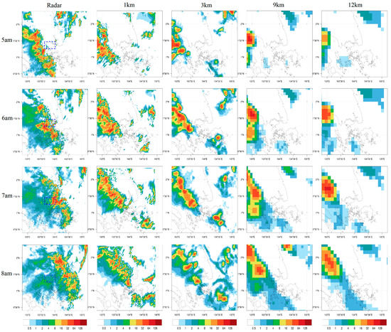
Figure 5.
Panel plot showing the rain intensity (mm/h) for the event on 4 November 2020 with a blue square outlining Singapore. Plotting limited to the 1 km domain extent. All times are local SGT (UTC + 8 h).
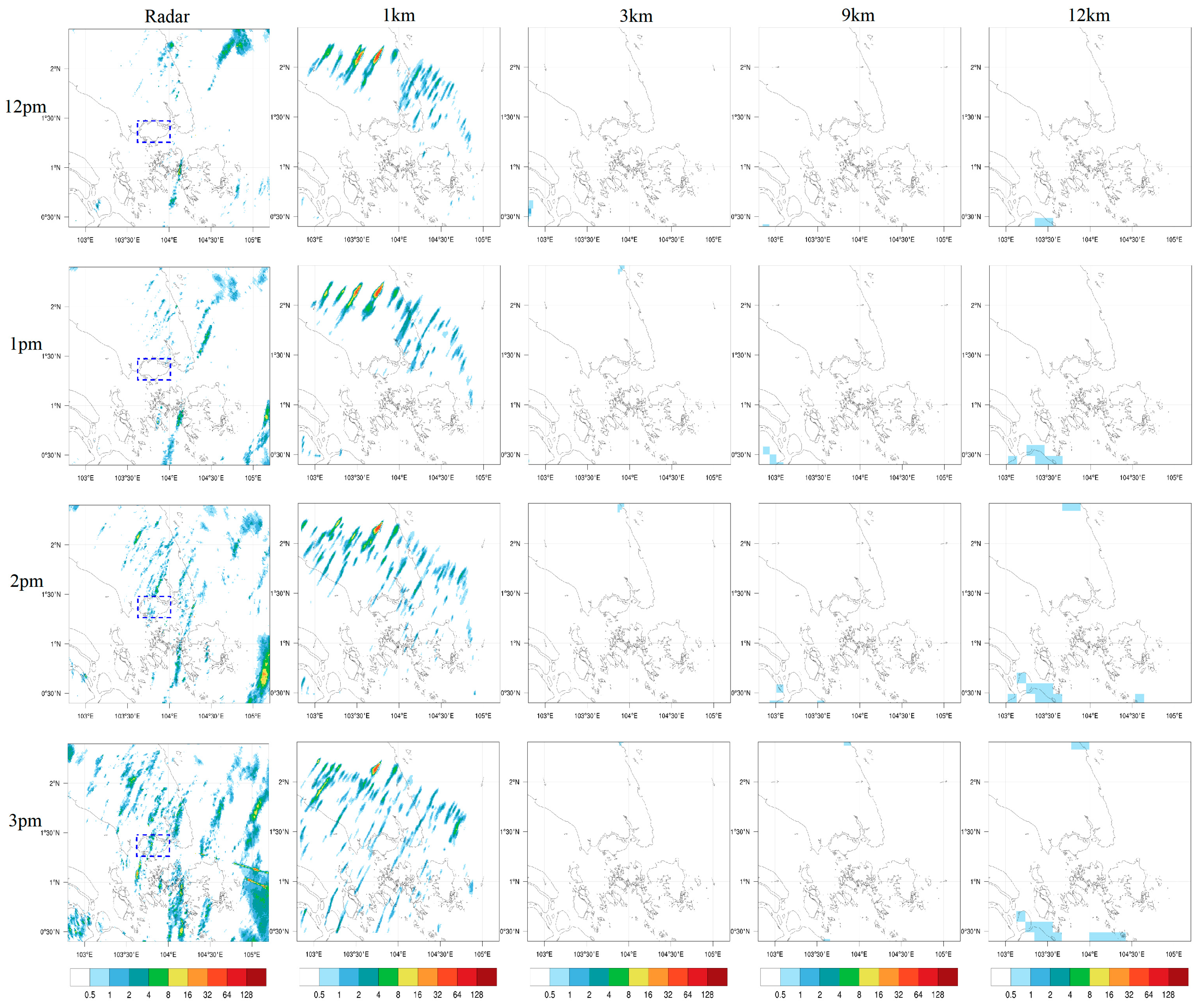
The 9 January 2021 event is a clear representation of the north-east monsoon showing the progression of rain bands from the north-east (Figure 6). What is very clear for this event is that only the 1 km domain is able to produce any rain over the Singapore region, albeit with some mismatch in the timing/location, with all other domains failing to spin-up any rain bands.

Figure 6.
Panel plot showing the rain intensity (mm/h) for the event on 9 January 2021 with a blue square outlining Singapore. Plotting limited to the 1 km domain extent. All times are local SGT (UTC + 8 h).
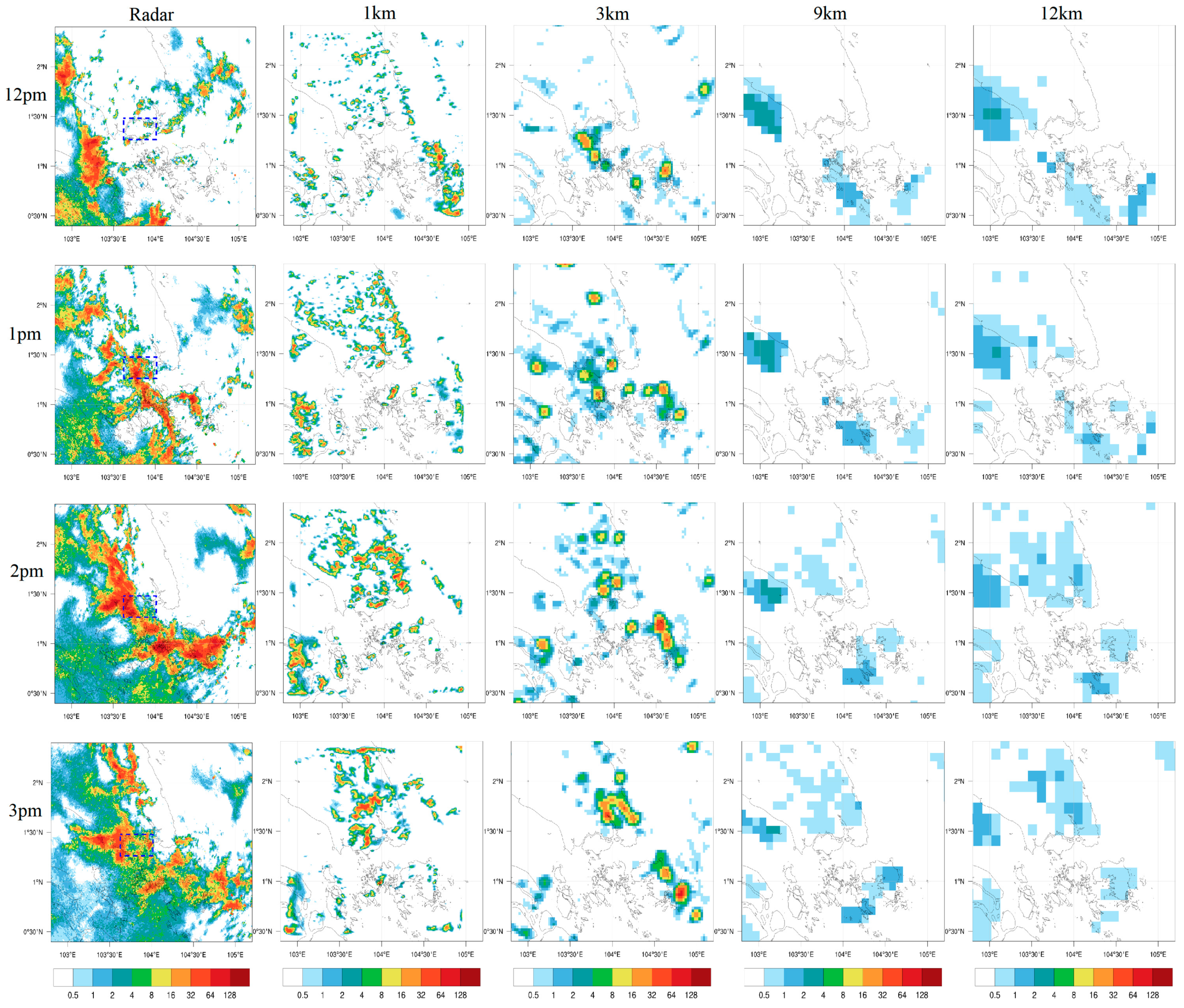
Finally, the 17 April 2021 event is also a squall line, however, occurring in the inter-monsoon season and later in the day (Figure 7). From midday local time, a large band of rain swept across Singapore resulting in, on average, 90 mm of rain in the space of 5–6 h. None of the WRF domains were able to capture the intensity or extent of the storm with only the 1 km and 3 km domains displaying some amount of heavy rain (Figure 7) and with the 1 km domain producing much higher HR and CSI when compared to the 3 km domain (Table 6).

Figure 7.
Panel plot showing the rain intensity (mm/h) for the event on 17 April 2021 with a blue square outlining Singapore. Plotting limited to the 1 km domain extent. All times are local SGT (UTC + 8 h).
3.2. Performance on Testing Set Compared to Radar-Derived Rain Rates
Comparison was also made against the radar-derived rain rates for both the contingency table metrics and the FSS. When measured against radar data, the contingency table metrics for the 15-day testing set tell a similar story to those derived from observations. From Figure 8, we see that the 1 km domain is the standout domain. However, the difference between the 1 km and other domains is much larger than the ground observation results (Figure 8). When using the radar as the ground truth, the 1 km domain has highest CSI for all rain rates and the 3 km domain suffers in performance with stark differences in the metrics between the 1 km and 3 km for all rain rates (Figure 8).

Figure 8.
As per Figure 4 but when using radar-derived rain rates as the ground truth. In (a), the HR, in (b), the FAR and in (c), the CSI for the 15-day testing set.
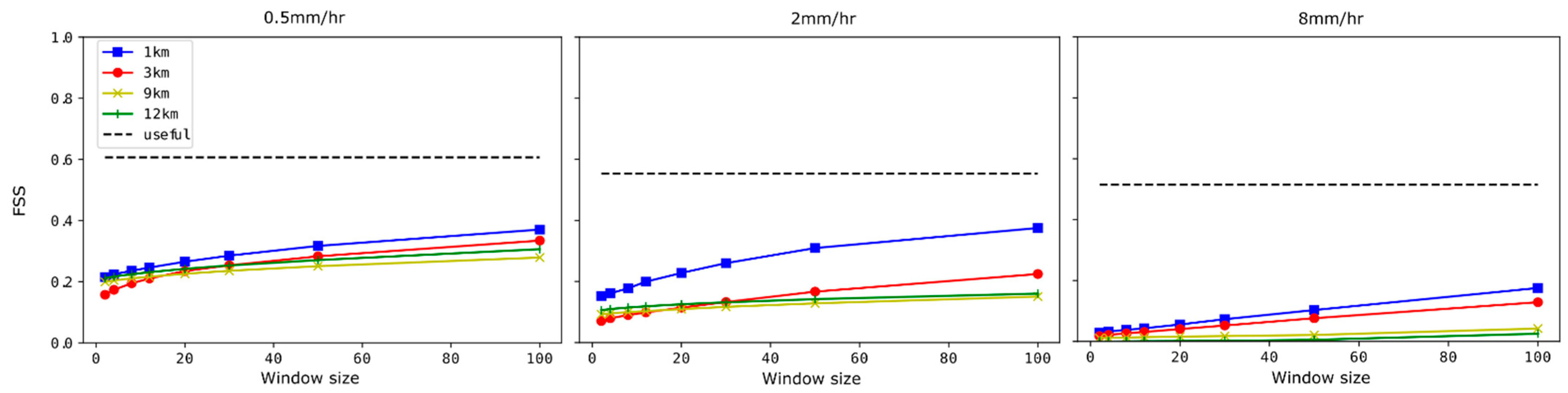
For the days highlighted in Section 3.1, the daily average of the hourly FSS was also calculated at various rain rates and neighbourhood sizes (windows). For the early morning heavy rain event on 4 November 2020, Figure 9 shows the FSS for 0.5, 2 and 8 mm/h and increasing window size. From Figure 9, it is evident that the 1 km domain had superior FSS for all rain rates. We also see that the 3 km domain had lower FSS at 2 mm/h, which was opposite to the CSI values in Table 4 where the 3 km domain had the highest CSI value. In addition, in Figure 9, we see the value of the FSS metric when compared to CSI. Relying on Table 4 only would suggest no skill at 9 km and 12 km grid size for higher rain rates, however, the FSS metrics are able to discern skill at higher rain rates and enable comparison with the other domains, as opposed to the CSI.
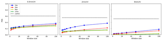
Figure 9.
Daily average FSS for various rain rates and window sizes for the 4 November 2020 event. is shown for each rainfall threshold with the dotted line.
Figure 10 shows the FSS metric for the 9 January 2021 north-east monsoon day. Contrary to the CSI results in Table 5, the 3 km domain was shown to have non-zero FSS values for the 9 January 2021 event, and for heavier rain rates, more skill than the 1 km domain, which was the only domain to show any skill in Table 5. However, for the light rain (0.5 mm/h) and larger window size, the 1 km domain did have higher FSS, which is more consistent with Figure 6 where the 1 km domain was able to forecast the lines of convection over Singapore. The small window skill scores were generally lower for this event indicating the difficulty in capturing the strong north-east flow (Figure 6).
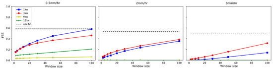
Figure 10.
As per Figure 9 but for the 9 January 2021 event.
For the 17 April 2021 event, we see mixed results using the FSS metric at 0.5 mm/h with the 12 km domain actually exhibiting the highest skill at the smallest window (Figure 11). However, heavier rain rates are more consistent with Table 6 and Figure 7, showing higher skill with finer grids and with the 1 km domain exhibiting the highest skill.
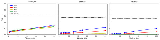
Figure 11.
As per Figure 9 but for the 17 April 2021 event.
3.3. Performance on 10 January 2021 Heavy Rain Event
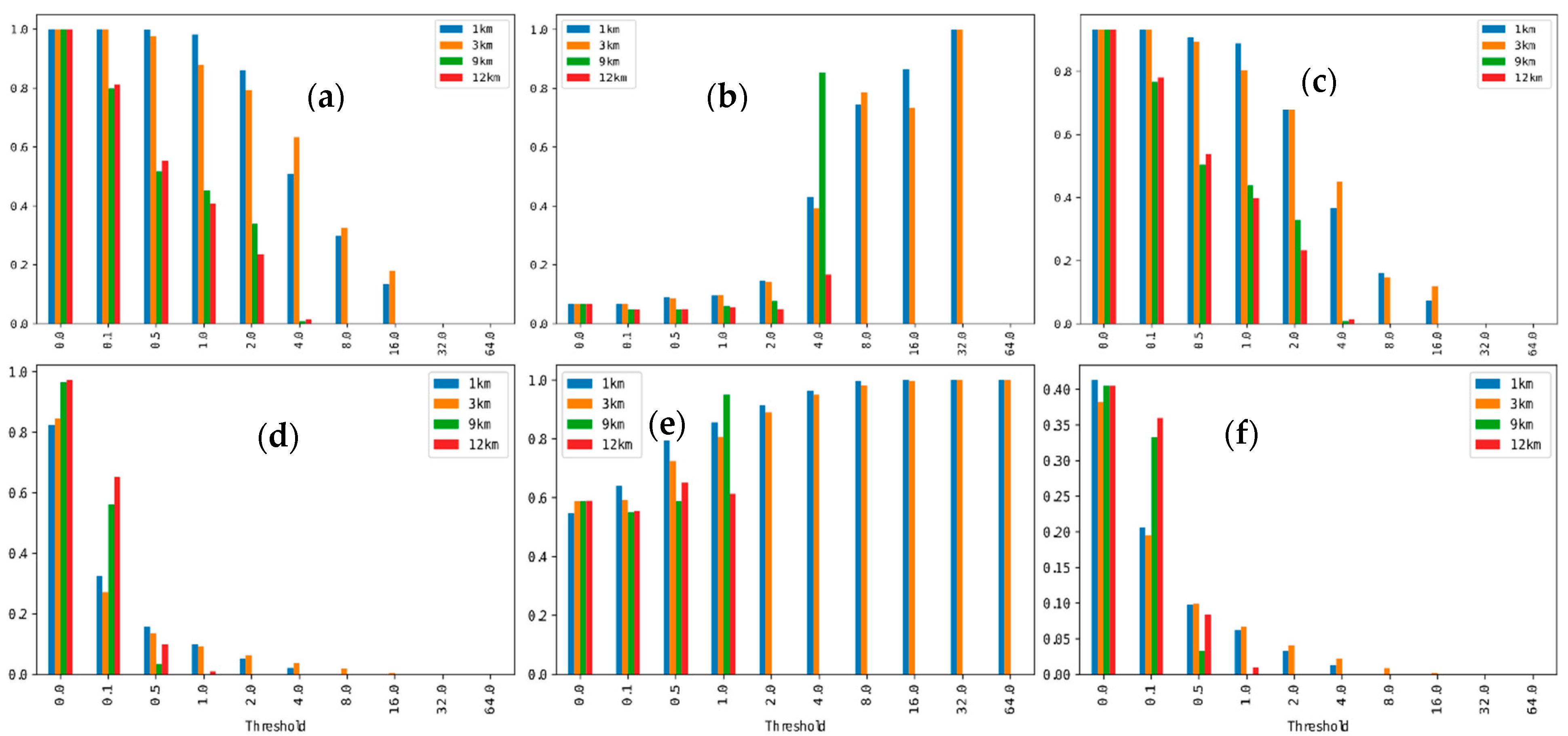
In this study, we also sought to analyse a particularly heavy rain day outside of the 15-day testing set. Figure 12 shows the performance of the various domains and rain rates for the 10 January 2021 heavy rain event when measured against ground observations in the top row and when measured against radar-derived rain rates in the bottom row. This event saw, on average, 105 mm of rain across the island and even up to 204 mm in one location. Contrary to the 15-day testing set and the other days that have been highlighted thus far, for the January 10 event, the 3 km domain performed the best for the heavier rain rates of 4 mm/h and 16 mm/h (Figure 8). When compared to the ground observation metrics, we see an overall decrease in the metrics (HR and CSI) for the radar-derived rain rates indicating a broader mismatch between the rain timing/location over the extended region.
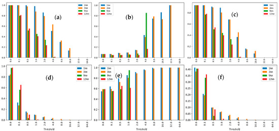
Figure 12.
Performance of various WRF spatial resolutions versus rainfall threshold for the 10 January 2021 heavy rain event. The top row of (a–c) are results measured against ground observations while (d–f) are results measured against the radar-derived rain rates. In (a,d) are the HR results, in (b,e) are the FAR results, and in (c,f) are the CSI.
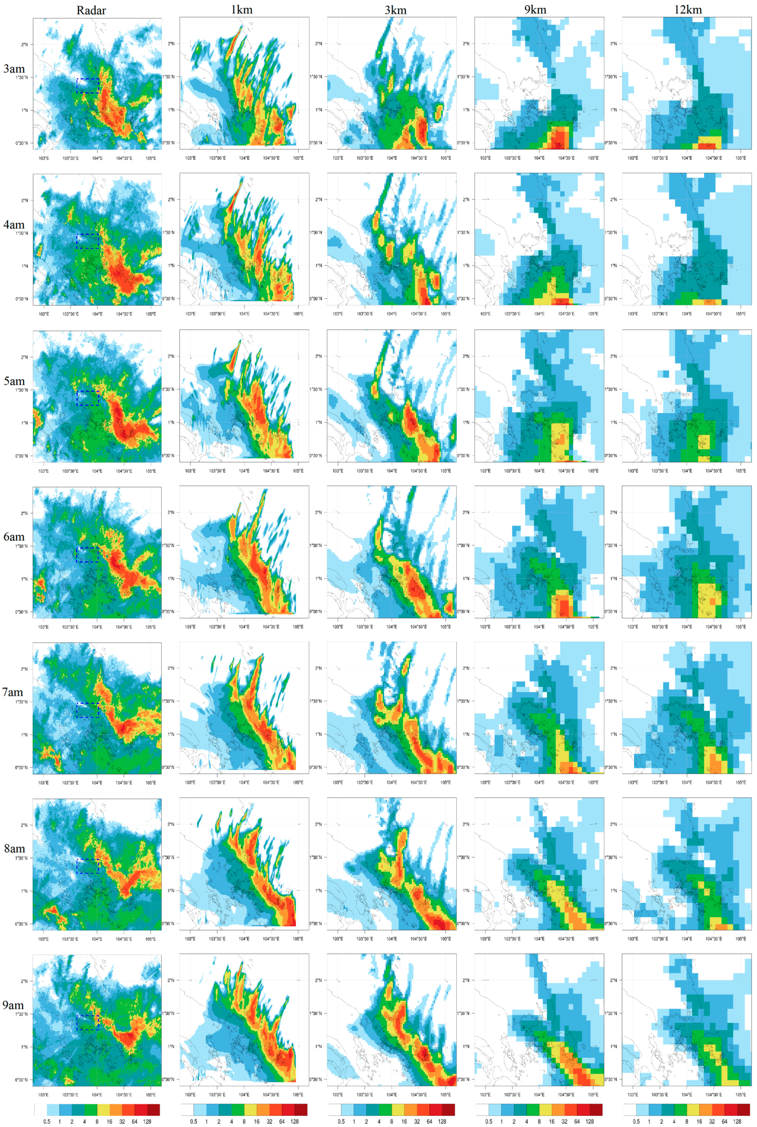
To analyse in more detail, Figure 13 shows comparisons with the radar images on 10 January 2021. From Figure 13, we see that the 1 km domain is able to produce heavier rain amounts but not necessarily in the right locations or at the right times. This tendency of the 1 km domain can clearly lead to larger amounts of false alarms. From Figure 13, we see that the largest differences in location and intensity between domains occur earlier in the simulation (i.e., 3 a.m., which is 7 h from initialisation), while later in the simulation, all domains tend to have a band of rain at or just east of Singapore with relatively good concordance with the radar.
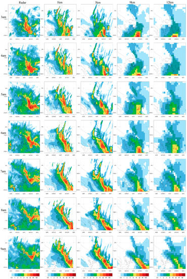
Figure 13.
Panel plot showing the rain intensity (mm/h) for the event on 10 January 2021 with a blue square outlining Singapore. Plotting limited to the 1 km domain extent. All times are local SGT (UTC + 8 h).
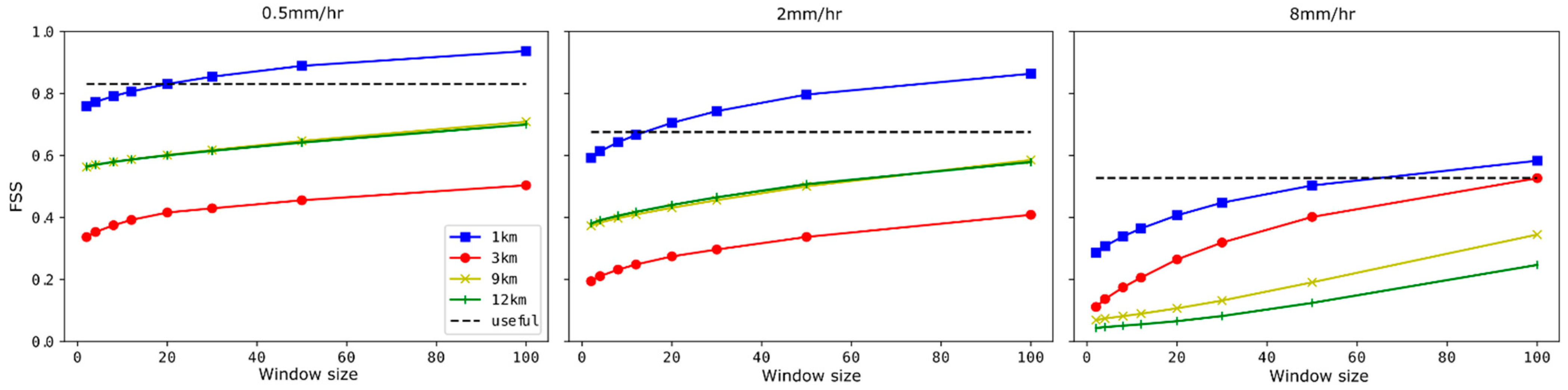
Finally, analysing the FSS metrics for the 10 January 2021 event shows that the 1 km domain was the standout performing domain (Figure 14). Interestingly, the 3 km domain showed relatively low FSS for the 0.5 mm/h and 2 mm/h rain rates. The FSS results were contrary to the contingency table metrics in Figure 12 where the CSI was relatively high for the 3 km domain at these rain rates.

Figure 14.
As per Figure 9 but for the 10 January 2021 event.
4. Summary and Conclusions
In this study, we have compared the rainfall performance of various WRF model domain resolutions (1 km, 3 km, 9 km and 12 km) over Singapore. We selected a representative set of 15 days with a mixture of seasons, types of rain events and rain amounts. On the testing set, we showed that the highest resolution (1 km) had the best performance (highest CSI) for rain rates above 0.5 mm/h and when compared to ground observations. This result was then confirmed when comparison was made against radar-derived rain rates. We showed the coarser domains had better overall performance at the lower rain rates when ground observations were used as the truth, but when analysing certain days in more detail, it was clear that the coarser domains were unable to correctly capture any of the heavier rain rates (particularly the 9 km and 12 km domains above 2 mm/h). Additionally, we calculated the Fractions Skill Score (FSS) for three highlighted days over the testing set and showed that, in general, the 1 km domain exhibited highest skill for the heavier rain events. We then analysed a particularly heavy rain day not from the original 15-day set. The 10 January 2021 heavy rain day saw in excess of 100 mm of rain on average across the island of Singapore. On this day, the 3 km domain had highest CSI for the heavier rain rates at 4 mm/h and 16 mm/h—contrary to the 15-day set. However, the FSS showed highest skill from the 1 km domain, which was concordant with a visual inspection of the event. In general, we found the 1 km domain to be able to capture the most realistic-looking features and heaviest rain amounts. This is reflected in the FSS values, but the timing and location can be incorrect leading to lower hits, higher false alarms and thus lower CSI. We also found that all domains tended to experience the same level of mismatch in the onset of rainfall indicating the cause is likely downstream of the global model input (ECMWF). In order to rectify this issue, special attention is needed in either the assimilation of local data or the inclusion of other global model inputs in an ensemble.
Author Contributions
Conceptualization, R.H. and G.S.; methodology, R.H.; formal analysis, R.H.; investigation, R.H.; resources, G.S.; data curation, R.H. and G.S.; writing—original draft preparation, R.H.; writing—review and editing, G.S.; visualization, R.H.; supervision, G.S.; project administration, G.S.; funding acquisition, G.S. All authors have read and agreed to the published version of the manuscript.
Funding
This study was funded by Envision Digital International Pte Ltd.
Data Availability Statement
Where reasonable, the authors will provide data utilised in this study.
Acknowledgments
The authors acknowledge Envision Digital International Pte Ltd. for funding the research, the European Centre for Medium-Range Weather Forecasts for the data used to drive the WRF model and the Huawei Cloud supercomputer where the simulations were run. We also acknowledge Nathan Eizenberg for the Python code to calculate the fast FSS. This code was downloaded from https://github.com/nathan-eize/fss, accessed on 6 April 2022. The authors would also like to thank the reviewers for taking the time to thoroughly read the paper and give useful suggestions to improve the manuscript.
Conflicts of Interest
The authors declare no conflict of interest.
References
- Svetlana, D.; Radovan, D.; Ján, D. The Economic Impact of Floods and their Importance in Different Regions of the World with Emphasis on Europe. Procedia Econ. Financ. 2015, 34, 649–655. [Google Scholar] [CrossRef] [Green Version]
- Gulev, S.K.; Thorne, P.W.; Ahn, J.; Dentener, F.J.; Domingues, C.M.; Gerland, S.; Gong, D.; Kaufman, D.S.; Nnamchi, H.C.; Quaas, J.; et al. 2021: Changing State of the Climate System. In Climate Change 2021: The Physical Science Basis. Contribution of Working Group I to Sixth Assessment Report of the Intergovernment Panel on Climate Change; Cambridge University Press: Cambridge, UK, in press; Available online: https://www.ipcc.ch/report/ar6/wg1/downloads/report/IPCC_AR6_WGI_Chapter_02.pdf (accessed on 6 April 2022).
- Seneviratne, S.I.; Zhang, X.; Adnan, M.; Badi, W.; Dereczynski, C.; Di Luca, A.; Ghosh, S.; Iskandar, I.; Kossin, J.; Lewis, S.; et al. 2021: Weather and Climate Extreme Events in a Changing Climate. In Climate Change 2021:The Physical Science Basis. Contribution of Working Group I to Sixth Assessment Report of the Intergovernment Panel on Climate Change; Cambridge University Press: Cambridge, UK, in press; Available online: https://www.ipcc.ch/report/ar6/wg1/downloads/report/IPCC_AR6_WGI_Chapter_11.pdf (accessed on 6 April 2022).
- Ayzel, G.; Heistermann, M.; Sorokin, A.; Nikitin, O.; Lukyanova, O. All convolutional neural networks for radar-based precipitation nowcasting. Procedia Comput. Sci. 2019, 150, 186–192. [Google Scholar] [CrossRef]
- Zhang, F.; Wang, X.; Guan, J.; Wu, M.; Guo, L. Rn-net: A deep learning approach to 0–2 h rainfall nowcasting based on radar and automatic weather station data. Sensors 2021, 21, 1981. [Google Scholar] [CrossRef] [PubMed]
- Manandhar, S.; Lee, Y.H.; Meng, Y.S.; Yuan, F.; Ong, J.T. GPS-Derived PWV for rainfall nowcasting in tropical region. IEEE Trans. Geosci. Remote Sens. 2018, 56, 4835–4844. [Google Scholar] [CrossRef]
- Skamarock, W.C.; Klemp, J.B. A time-split nonhydrostatic atmospheric model for weather research and forecasting applications. J. Comput. Phys. 2008, 227, 3465–3485. [Google Scholar] [CrossRef]
- Jeworrek, J.; West, G.; Stull, R. WRF Precipitation Performance and Predictability for Systematically Varied Parameterizations over Complex Terrain. Weather Forecast. 2021, 36, 893–913. [Google Scholar] [CrossRef]
- Woodhams, B.J.; Birch, C.E.; Marsham, J.H.; Bain, C.L.; Roberts, N.M.; Boyd, D.F. What is the added value of a convection-permitting model for forecasting extreme rainfall over tropical East Africa? Mon. Weather Rev. 2018, 146, 2757–2780. [Google Scholar] [CrossRef]
- Dipankar, A.; Webster, S.; Sun, X.; Sanchez, C.; North, R.; Furtado, K.; Wilkinson, J.; Lock, A.; Vosper, S.; Huang, X.-Y. SINGV: A convective-scale weather forecast model for Singapore. Q. J. R. Meteorol. Soc. 2020, 146, 4131–4146. [Google Scholar] [CrossRef]
- Jolivet, S.; Chane-Ming, F. WRF Modelling of Turbulence Triggering Convective Thunderstorms over WRF Modelling of Turbulence Triggering Convective Thunderstorms over Singapore. In Turbulence and Interactions; Deville, M., Estivalezes, J.L., Gleize, V., Lê, T.H., Terracol, M., Vincent, S., Eds.; Notes on Numerical Fluid Mechanics and Multidisciplinary Design; Springer: Berlin/Heidelberg, Germany, 2014; Volume 125, pp. 115–122. [Google Scholar] [CrossRef]
- Clark, P.; Roberts, N.; Lean, H.; Ballard, S.P.; Charlton-Perez, C. Convection-permitting models: A step-change in rainfall forecasting. Meteorol. Appl. 2016, 23, 165–181. [Google Scholar] [CrossRef] [Green Version]
- Sangati, M.; Borga, M. Influence of rainfall spatial resolution on flash flood modelling. Nat. Hazards Earth Syst. Sci. 2009, 9, 575–584. [Google Scholar] [CrossRef] [Green Version]
- Moya-Álvarez, A.S.; Martínez-Castro, D.; Kumar, S.; Estevan, R.; Silva, Y. Response of the WRF model to different resolutions in the rainfall forecast over the complex Peruvian orography. Theor. Appl. Climatol. 2019, 137, 2993–3007. [Google Scholar] [CrossRef]
- Roberts, N.M.; Lean, H.W. Scale-Selective Verification of Rainfall Accumulations from High-Resolution Forecasts of Convecive Events. Mon. Weather Rev. 2008, 136, 78–97. [Google Scholar] [CrossRef]
- Faggian, N.A.T.H.A.N.; Roux, B.; Steinle, P.; Ebert, B. Fast calculation of the fractions skill score. Mausam 2015, 66, 457–466. Available online: https://metnet.imd.gov.in/mausamdocs/166310_F.pdf (accessed on 6 April 2022). [CrossRef]
- Mittermaier, M.; Roberts, N. Intercomparison of Spatial Forecast Verification Methods: Identifying Skillful Spatial Scales Using the Fractions Skill Score. Weather Forecast. 2010, 25, 343–354. [Google Scholar] [CrossRef]
- Huva, R.; Song, G.; Zhong, X.; Zhao, Y. Comprehensive physics testing and adaptive WRF physics for day-ahead solar forecasting. Meteorol. Appl. 2021, 28, 1–13. [Google Scholar] [CrossRef]


Publisher’s Note: MDPI stays neutral with regard to jurisdictional claims in published maps and institutional affiliations. |
© 2022 by the authors. Licensee MDPI, Basel, Switzerland. This article is an open access article distributed under the terms and conditions of the Creative Commons Attribution (CC BY) license (https://creativecommons.org/licenses/by/4.0/).