The December 2021 Marshall Fire: Predictability and Gust Forecasts from Operational Models

Abstract

We analyzed meteorological conditions that occurred during the December 2021 Boulder, Colorado, downslope windstorm. This event is of particular interest due to the ignition and spread of the Marshall Fire, which quickly became the most destructive wildfire in Colorado history. Observations indicated a rapid onset of fast winds with gusts as high as 51 m/s that generally remained confined to the east-facing slopes and foothills of the Rockies, similar to previous Boulder windstorms. After about 12 h, the windstorm shifted into a second, less intense phase. Midtropospheric winds above northwestern Colorado weakened prior to the onset of strong surface winds and the event strength started waning as stronger winds moved back into the area. Forecasts from NOAA high-resolution operational models initialized more than a few hours prior to windstorm onset did not simulate the start time, development rate and/or maximum strength of the windstorm correctly, and day-ahead runs even failed to develop strong downslope windstorms at all. Idealized modeling confirmed that predictability was limited by errors on the synoptic scale affecting the midtropospheric wind conditions representing the Boulder windstorm’s inflow environment. Gust forecasts for this event were critically evaluated.

1. Introduction

The Marshall Fire reportedly started at approximately 11 am local time (1800 UTC) on 30 December 2021, near the intersection of state highways 93 and 170 in Boulder County, Colorado, about 7.8 km southeast of Boulder proper [1]. The incident appears to have been a “perfect storm” of fast winds and drought conditions as the combination of historically warm temperatures and low precipitation along the Front Range of the Rocky Mountains left the grasses in a state of extreme dryness [2]. The fire spread quickly eastward, driven by strong, westerly winds. By 12:15 local time (1915 UTC), the flame front had reached Cherokee Avenue in the town of Superior [1]. The fire subsequently burned through the towns of Superior and Louisville, reportedly leaving one dead, one missing, and injuring six others [3,4]. The fire also destroyed 1091 buildings [5], making it the most destructive in state history [6].

The fire occurred during a downslope windstorm, a weather event consisting of a “very strong, usually gusty, and occasionally violent wind that blows down the lee slope of a mountain range, often reaching its peak strength near the foot of the mountains and weakening rapidly farther away from the mountains” [7]. These windstorms occur worldwide and carry names such as “bora”, and “foehn” [8,9,10], and they play important roles in the weather phenomena known as “Diablo”, “Santa Ana”, and “Sundowner” winds in California [11,12,13]. When they occur along the Front Range, these windstorms are often called “chinooks”, popularly misunderstood to be a Native American word for “snow eater” [14]. Downslope windstorms occur frequently in the Boulder area, often producing strong, damaging winds [15,16,17]. According to NOAA (see abbreviations and acronyms list), 262 cases of >30 m/s windstorms have occurred in Boulder between 1969 and 2021 [18].

Downslope windstorms have been implicated in starting and/or spreading many wildfires in the western United States, including the Northern California Camp fire [19,20], the Cedar, Witch, and Thomas fires of Southern California [21,22,23], fires in the Santa Barbara area [24], the 2020 Labor Day fires in the Pacific Northwest [25], and fires in the Boulder area [26,27], to name but a few. As a consequence, accurate forecasts are critical for many reasons, including situational awareness, informing public safety power shutoffs [28], and driving fire spread modeling efforts [29,30,31,32]. However, the predictability of downslope windstorms can be limited. Subtle variations in environmental conditions can lead to significantly different outcomes with respect to magnitude, structure, and/or even the development of strong winds at all [33,34]. In numerical simulations, sensitivities to model resolution, initial conditions, and numerical details have been identified [35,36,37,38,39]. Model physical parameterizations play an important role in forecast skill for many important variables, especially wind speed and direction [24,39,40,41].

Of interest here is the lead time regarding the Marshall fire event available to forecasters, emergency planners, fire-management decision makers, first responders, and public utilities owing to high-resolution numerical weather prediction guidance. NOAA operates two models with horizontal grid spacings of 3 km: the HRRR and the NAM-HIRES CONUS (hereafter “NAM”) nest. These models differ with respect to their dynamical cores, model physics, boundary conditions, initialization strategies, and data assimilation details, so they provide two quasi-independent views of the windstorm event. On the basis of HRRR forecast cycles initiated between 00 and 09 UTC on 30 December, the National Weather Service (NWS) office in Boulder issued a High Wind Warning for the foothills of Boulder and Jefferson counties at 1036 UTC on that date (Paul Schlatter, personal communication, 2022).

However, this warning came less than 5 h prior to the start of the wind event, and only about 9 h prior to its peak. We will show that the HRRR and NAM forecast skill degraded rather swiftly with increasing lead time in this case. Our analysis will point to subtle position inaccuracies involving a midtropsopheric shear zone resulting in significant errors in representing conditions over western Colorado, leading to delayed or even absent development of strong surface winds in the foothills between Boulder and Denver. We will also examine gust products from these models. While verifications of surface and boundary layer winds and temperatures have been made, at least for the HRRR [42,43,44,45,46], the gust products these models generate have received much less attention.

The structure of this paper is as follows. Section 2 outlines materials and methods. Section 3 discusses the available surface observations, the synoptic overview, and conditions existing upwind of Boulder before and during the windstorm episode. Section 4 reviews the forecasts from the operational HRRR and NAM models, and documents the decline in skill with increasing lead time, while Section 5 evaluates a hypothesis for that skill degradation. Section 6 examines gust forecasts from the operational models. The final section presents a summary and discussion of results.

2. Materials and Methods

Our analyses made use of gridded operational forecast products produced by NOAA that may be obtained from Amazon Web Services and Google Cloud via the NOAA Big Data Program. Observational data were obtained from MADIS, supplemented by 10 m wind information from the National Renewable Energy Laboratory’s National Wind Technology Center (NWTC). Only publicly available observations were used. We employed software made available and supported by the Developmental Testbed Center, including the Model Evaluation Tools (MET) and the Unified Post Processor (UPP). Graphics were created using the Matplotlib and Cartopy Python packages. See Data Availability section for more information.

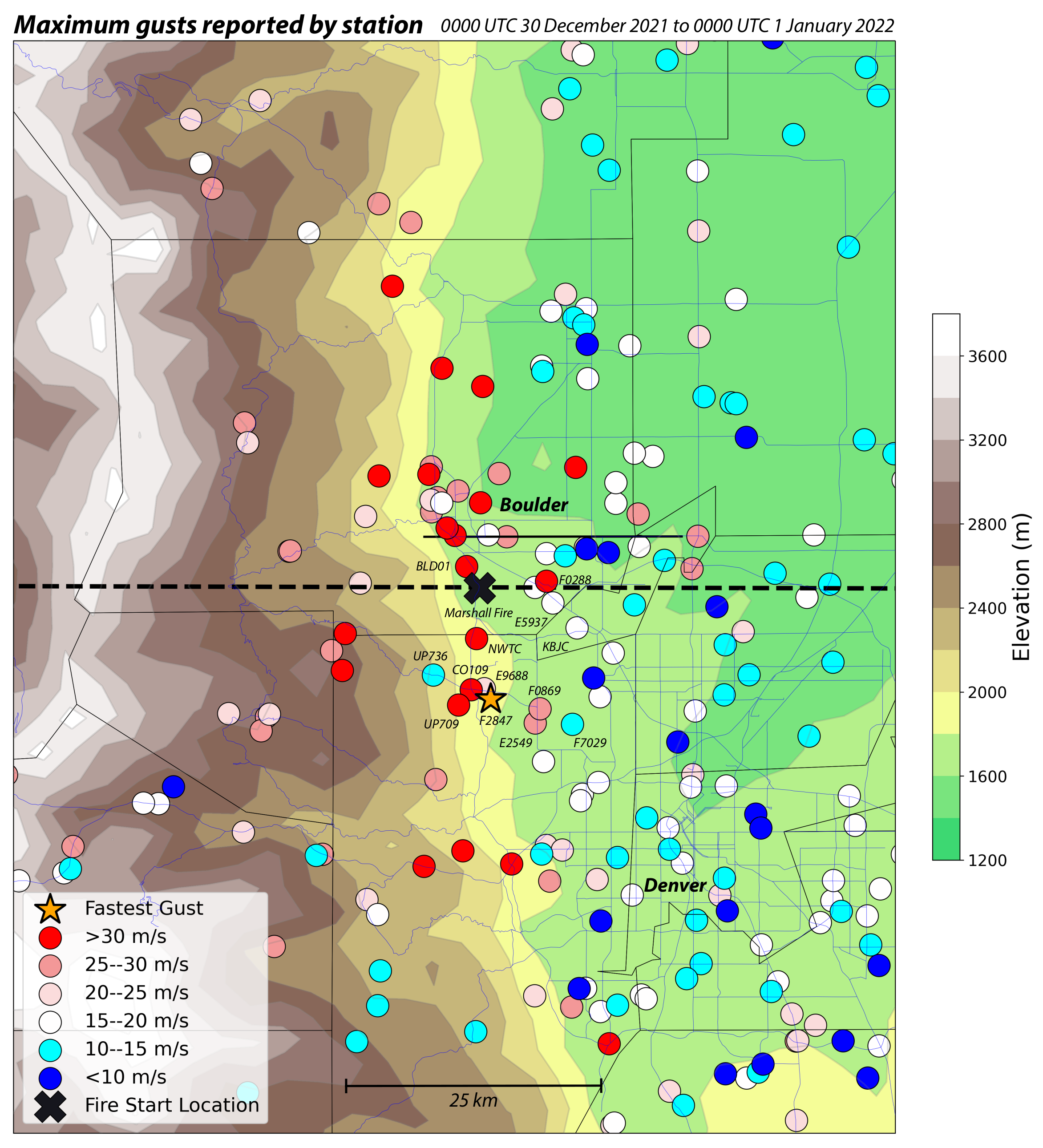
3. Surface Gust Observations and Synoptic Situation

3.1. Observations

Surface observations for typical measurements (sustained wind speed and direction, gust, dry bulb and dew point temperatures, and relative humidity) were obtained from MADIS and examined for reasonableness. Available sites represented a mix of networks including ASOS and AWOS (mainly airport), RAWS (typically on terrain slopes), mesonet stations (such as those operated by the Colorado Department of Transportation, or CDOT), and privately-owned sites (members of APRSWXNET). Comparisons are somewhat impeded by variations in anemometer mounting height, exposure, and equipment type, site exposure and recording precision, and also reporting, sampling, and averaging intervals.

Figure 1 presents the maximum reported gusts in the database within a 2-day time window commencing 0000 UTC 30 December 2021 that were retained for this analysis. It is seen that the highest speeds (colored red) were concentrated into a fairly narrow band close to the Front Range. The largest gusts were recorded just south of the apparent Marshall fire ignition site (indicated by the “X”) at a trio of stations separated by no more than 3.2 km. APRSWXNET station F2847 (marked by the star) reported the highest gust, 51.4 m/s [115 mph], at both 1906 and 1911 UTC on 30 December. This station, which is about 11 km south of the Marshall ignition site, also had the third highest gust (49.2 m/s) a few minutes earlier (1856 UTC) and accounted for 13 of the top 18 gust reports in the state. The second-ranked site, CDOT station CO109, which is located 2.1 km west of F2847, provided the third-fastest gust report (49.0 m/s or 110 mph) at 1823 UTC 30 December and six of the 20 fastest readings. Close by is the third-ranked station, UP709 from the Union Pacific Railroad network, which recorded a 46 m/s gust at 2026 UTC.

Time series of surface observations for CO109, UP709, and F2847 (Figure 2) suggest the windstorm event commenced there around 1500 UTC 30 December, peaked between 1700 and 2000 UTC, and shifted into a weaker second phase after 0200 UTC 31 December. The event start at CO109 was marked by a sharp increase in temperature, winds, and gusts, accompanied by a steep drop in relative humidity (Figure 2a,b). The decline of wind and gust speeds during the second phase was less abrupt at UP709 (Figure 2c) than at CO109 or F2847 (Figure 2d), which are 1–3 km farther from the mountains, indicating that a shift in the spatial extent of the downslope winds occurred during the second phase. Temperature and humidity observations at CO109 (Figure 2a) reveal that this second phase ended on or before 1300 UTC 31 December, at which time a synoptic front passed.

Although wind and gust speeds at these three neighboring stations were fairly comparable, reported directions for the sustained winds were not. CO109 had westerly winds, as would be anticipated during a Front Range windstorm, but F2847 consistently reported very strong easterlies during the first phase. There is no evidence that this was a rotor, a potentially hazardous phenomenon that often occurs during downslope windstorms [10,47,48,49] and apparently did so elsewhere during this event [2], possibly having been captured at neighboring stations KBJC, E5937, and F0869 (see Figure 1). Although not shown, a comparison involving contemporaneous December 2021 observations with at least moderate sustained winds (>5 m/s) suggested that disagreements in wind direction between F2847 and CO109 were not uncommon, and thus the former’s wind direction, if not speed, information may be considered suspicious. That being said, event winds at UP709 were consistently from the southeast during the event, likely influenced by the local terrain, and the fact that three stations in close proximity reported the state’s strongest gusts during this event lends credence to these gust speeds.

3.2. Synoptic Situation

Figure 3 presents the 400 hPa wind and geopotential height fields at four selected times in the 24 h period between 1200 UTC on 30 and 31 December 2021. These fields represent analyses (i.e., zero-hour forecasts) from the GFS model, which are presumed to be correct, and the level selected will be seen as important in the following discussion. At 1200 UTC on 30 December (Figure 3a), a narrow, positively tilted trough was situated in the western United States extending from southwest to northeast. At this time, strong westerly winds were present across northern Colorado (CO). This is more easily seen in the inset, on which the star marks the Boulder area. However, there was substantial horizontal wind shear at the northern edge of the jet and subsequent shifting of this pattern brought significantly slower winds over northwestern Colorado by 1800 UTC (Figure 3b). As shown in Figure 2, the windstorm was ramping up at this time. Stronger 400 hPa winds were returning to the region by 0000 UTC 31 December (Figure 3c), which was past the event peak, and the event had effectively concluded by 1200 UTC 31 December (Figure 3d).

3.3. Conditions at and Upstream of Boulder

The HRRR is a convection-allowing model operating at 3 km grid spacing over the CONUS. As of December 2021, the model was based on WRF-ARW and used a terrain-following coordinate. New HRRR forecast cycles were being launched hourly and extended to 48 h for the 0000, 0600, 1200, and 1800 UTC runs; other cycles ran to 18 h [50]. HRRR forecast products were available both on isobaric and native (terrain-following) model levels. As the isobaric fields were subjected to substantial horizontal smoothing [51], only the native level outputs were used for our study.

The evolution of environmental conditions before and during the windstorm is illustrated by Figure 4a,b, which were constructed using hourly HRRR analyses. Panel (a) is for a location in western Colorado (identified on the Figure 3 insets and subsequent figures) about 90 km west of Boulder/Marshall, and selected to represent the inflow environment for Boulder, which is shown in Figure 4b. Prior to the approximate event start time of 1500 UTC 30 December (8 am local time), strong westerly winds (shaded field) were present upstream of Boulder through much of the troposphere, including the 400 hPa level previously examined (about 6900 m MSL). However, as hinted by Figure 3b, the appearance of strong downslope winds on the Front Range coincided with a substantial reduction in the westerly flow upwind of Boulder and the winds remained slower until the end of the first, stronger phase of the event around 0200 31 December (7 pm local time).

The potential temperature contours (isentropes) in Figure 4a provide information about atmospheric stability, which becomes larger as the vertical spacing decreases. During the course of the first phase, stability increased in the 4–6 km MSL layer relative to the environment’s pre-windstorm condition, and was especially high around the time of the event peak (vertical black dashed line). Simultaneously, lower tropospheric stability decreased in conjunction with daytime heating. The aforementioned long decline in winds occurred as wind speeds in the middle and upper troposphere increased and the boundary layer became more stable after sunset, which occurred around 0000 UTC.

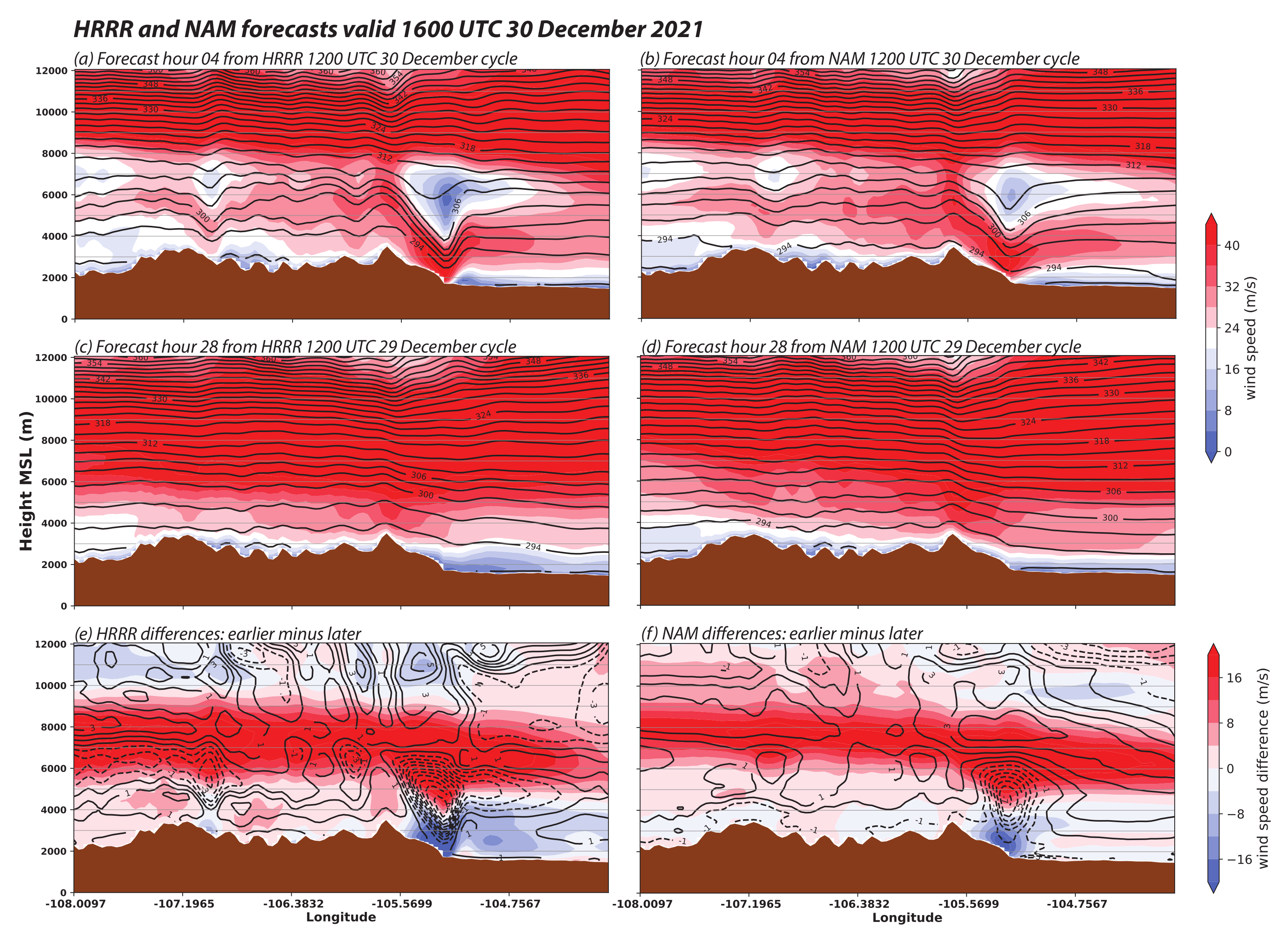
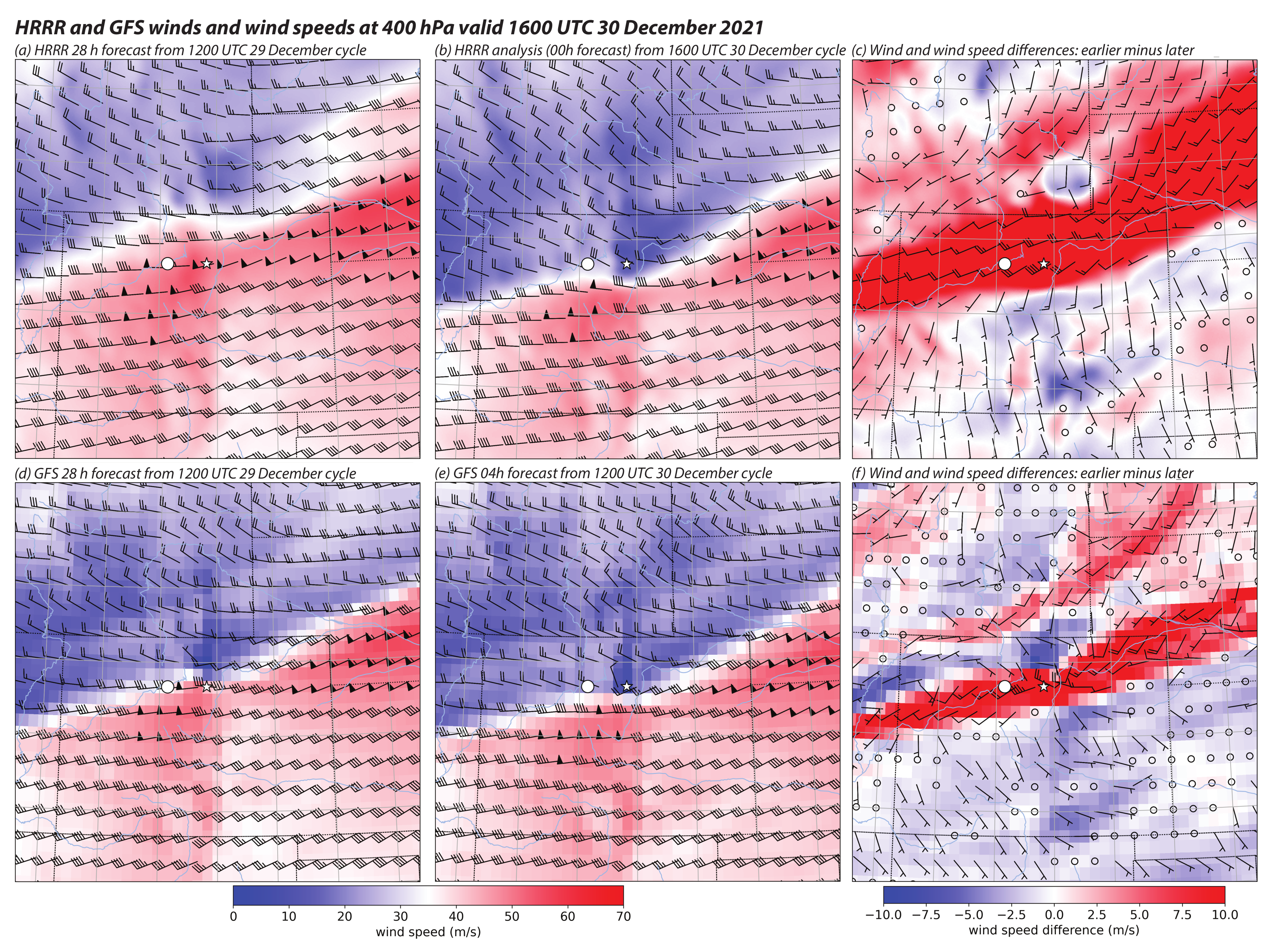
4. Operational Forecasts

The HRRR cycle commencing 1200 UTC on 30 December captured the evolution of the wind event well with respect to timing and intensity. Figure 5 shows vertical cross-sections oriented west–east across the Marshall fire ignition point (see Figure 1 for cross-section orientation) for four times during this model run. At 1400 UTC 30 December (forecast hour 2), we see a very weak downslope event with the fastest winds in the lower troposphere located above the ≈3.7 km MSL peak in this cross-section and the isentropes gently curved downward. By 2000 UTC the same day (Figure 5b), near the event peak according to Figure 2 and after the fire started, fast winds were being predicted on the east-facing slope and extending eastward across the fire location (labeled on panel b) before lofting. In the middle troposphere above the rapidly descending airflow, winds were weak and potential temperature well-mixed as in classic severe downslope windstorms around the world, including Boulder [52,53,54]. Consistent with the observations (Figure 1), the model was not forecasting strong surface winds extending much beyond the immediate Boulder area. By the end of the first phase (0200 UTC 31 December, Figure 5c), near-surface wind speeds were predicted to have become significantly weaker as well as even more confined to the lee slope, and by 1000 UTC (F22, Figure 5d) the situation was forecast to return to fairly weak winds that did not reach the surface.

In Figure 6, observed gusts (in red) at CO109 are compared to HRRR forecasts from various lead times of “gust potential”, created using boundary layer depth and wind predictions as described in [51]. The forecasts shown came from top-of-hour outputs interpolated to the station location. According to [51], the gust potential is expected to “often exceed the observations of transient wind gusts at a particular time”. For this event, the forecasts from the 1200 UTC 30 December HRRR run (in black) captured the evolution of the event’s first phase quite well, although it underpredicted the fastest reported gusts across the event peak.

While the 1200 UTC 30 December cycle provided skillful guidance regarding the evolution of the event, at longer lead times the HRRR was less successful in predicting the timing and/or strength of the gusts, not only at CO109 (Figure 6) but also at other stations in the Boulder area (not shown). The cycles that started at 0006 and 0000 UTC 30 December (in grey and brown, respectively) were noticeably late in developing strong gusts at CO109, although they indicated the actual event’s peak time satisfactorily. In the HRRR run from 1800 UTC the previous day (in green), 21 h prior to the event onset, the simulated event ramp-up was even slower and a later peak time was predicted. The 1200 UTC 29 December cycle (in blue) developed only a rather weak downslope windstorm during the event period, perhaps one that would have been viewed as unremarkable by forecasters and and other users of these numerical weather prediction products.

Figure 7a,b show vertical cross-sections from the HRRR valid at 1600 UTC 30 December, about an hour after event onset, from the 1200 UTC 30 December (4 h forecast) and 1200 UTC 29 December (28 h forecast) HRRR cycles. The cross-sections have been shifted westward relative to those of Figure 5 to reveal more of the higher elevation, upstream environment. At the longer lead time, the HRRR failed to develop strong, downslope winds in the Boulder area and the difference field (Figure 7c) emphasizes substantial discrepancies in forecast wind speed that existed particularly in the 5–9 km MSL layer west of Boulder, which includes the 400 hPa level examined earlier. This is not an HRRR problem, however, as forecasts from the 3-km NAM model (Figure 7, right column) were very similar to those from the HRRR.

Something was limiting the forecast skill from both high-resolution models. We note that neither model evolved the horizontal shear zone examined in Figure 3 perfectly. We will demonstrate that the resulting subtle position inaccuracy caused significant errors in representing conditions over western Colorado, upstream of Boulder, at longer lead times that directly controlled the models’ ability to develop a realistic and timely windstorm along the Front Range between Boulder and Denver. As this occurred similarly in the HRRR and the NAM, we will focus on the former.

Figure 8 presents HRRR wind and wind speed fields at the 400 hPa level valid at 1600 UTC 30 December 2021, representing the 1200 UTC 29 December cycle’s 28 h forecast (panel a) and the corresponding 00 h analysis (panel b), which is presumed more correct. Note that a relatively small difference in the synoptic pattern between the forecast and analysis has resulted in a substantial change in wind speeds across much of the CONUS, including northern Colorado. This is readily apparent on the wind difference plot (panel c), which subtracts the analysis time wind barbs and speeds from those of the 28 h forecast. Figure 9 (top row) affords a closer view of these fields. The stars represent Boulder and the white dots mark the location used for the upstream environment in Figure 4, left column.

The evolution of the wind and potential temperature fields for the 1200 UTC 29 December simulation are also shown in Figure 4. Owing to the pattern position error at this lead time, the middle tropospheric winds in the inflow environment did not diminish (Figure 4c), not only at the 400 hPa level but through a deep layer, and the windstorm at Boulder was both delayed in starting and considerably weaker in strength (Figure 4d). This is evident in the difference fields (Figure 4e,f), again representing the subtraction of the analysis from the 28 h forecast. Temperature differences (black contours) during the event indicate that the atmospheric conditions west of Boulder were predicted for the 28 h lead time to be less stable in the 3.5–7.5 km MSL layer through much of the event period. Discrepancies are negative overlying positive, indicating the expectation of a steeper lapse rate from the longer lead time prediction.

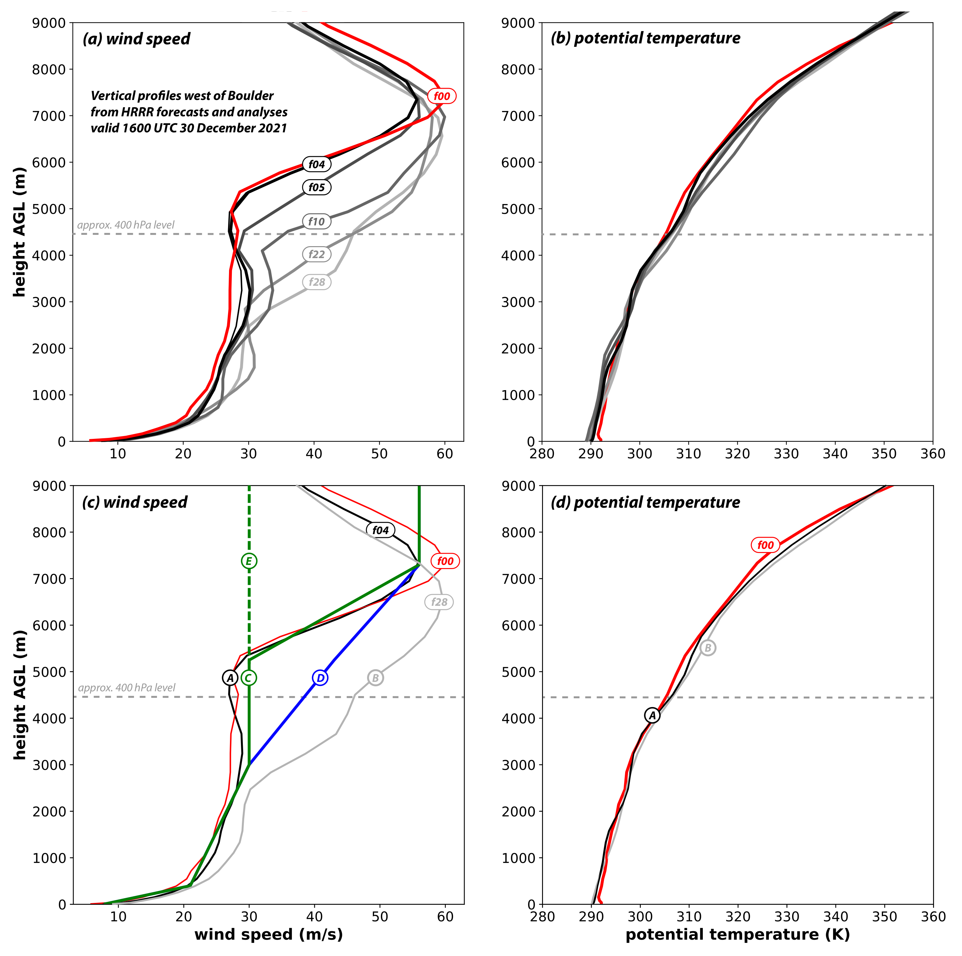
5. The Role of the Inflow Environment

The forecast gusts for station CO109 previously suggested that predictions of the timing and strength of the downslope winds became more accurate as the event start time approached. It has been well-established that windstorm behavior can be very sensitive to the structure of the inflow environment [34,36,38]. Figure 10 documents the temporal evolution of the inflow environment as constructed from HRRR analyses (top panel) as well as that predicted from earlier cycles. As seen previously, HRRR analyses reveal that wind speeds west of Boulder diminished through a deep layer around the time of the event start and remained relatively low until the end of the first, strong phase of the event. The 1200 UTC 30 December captured this evolution rather well (Figure 10b).

We have shown, however, that problems with evolving the synoptic pattern at longer lead times led to errors in timing and magnitude of the strong winds along the Front Range between Boulder and Denver. The HRRR’s 0600 and 0000 UTC cycle on 30 December started the windstorm late at CO109 (Figure 6) and Figure 10c,d reveal that the deep, strong westerly winds in the upstream environment were predicted to persist for a longer period of time in those model runs. The 1800 UTC 29 December run was even more delayed and we see its upstream winds did not slow until around the time of the actual event’s peak (Figure 10e). As previously seen, the 1200 UTC 29 December cycle failed to develop strong downslope winds at all. The evolution of western Colorado wind speeds in that cycle was even more unrealistic.

Figure 11 superimposes vertical profiles of wind speed and potential temperature for our selected upstream location from various HRRR model runs, all valid at 1600 UTC 30 December. (While total horizontal wind speed is being shown, the north–south component was small at this location, for all heights and times depicted.) Note that as the lead time shortened, forecast wind speeds diminished considerably, particularly in the 2.5–7 km AGL layer, as anticipated from Figure 10. By the 4 h lead (f04), the profile was quite similar to that of the analysis (f00). In contrast, the evolution of the potential temperature profile for the upstream environment was rather more subtle.

We hypothesize that errors in the representation of the upwind environment caused the models to fail to develop the windstorm properly with respect to timing and magnitude and that this was a direct consequence of the models’ inability to accurately translate the synoptic-scale pattern. Furthermore, we suspect that this behavior was controlled primarily by the wind profiles and specifically by the strength of the westerlies in the middle troposphere as those changes were the most profound. To test these hypotheses, we employed the wind and temperature profiles from Figure 11 as inputs to two-dimensional simulations made using the CM1 model [55]. Similar to [56], the model was configured with a bell-shaped “Witch of Agnesi” mountain with a height of 1.6 km, a rough proxy for height difference between the peak in the cross-sections shown in Figure 5 and Figure 7 and the Boulder area, and with a half-width of 25 km, which roughly conforms to the east-facing slope of the Front Range as rendered in the HRRR model. There are numerous differences between the idealized setup and the operational model, not the least of which being the topographic depiction, but this proxy helps us evaluate our hypotheses.

We start with the profiles from the 1200 UTC 30 December run’s f04, and the 1200 UTC 29 December run’s f28, which for convenience will be called profiles “A” and “B” as indicated on Figure 11’s bottom row. The fields presented in Figure 12 represent the CM1 runs’ 4 h forecasts, by which time an approximately steady state had been reached. As anticipated, inflow environment A (panel a) supported a downslope windstorm with some resemblance to what occurred in the HRRR model following event onset (Figure 7a). In both, the strongest surface winds occurred at the foothills, which was followed downwind by a hydraulic jump-like feature that left wind speeds farther from the peak being rather slow. In contrast, profile B failed to generate strong surface winds (panel b). Similar to what transpired in the 1200 UTC 29 December HRRR run that provided these profiles (Figure 7b), the fastest winds appeared at the peak and only weak descent of the isentropes over the east-facing slope occurred.

Panels (c) and (d) in Figure 12 evaluate whether the windstorm was more controlled by the wind or temperature structure. When the winds from A were used with profile B’s temperatures (panel c), a windstorm was still produced, one that was quite similar to that seen in Figure 12a. However, using profile A’s temperatures with B’s winds still failed to produce a strong windstorm (panel d). This result suggests that shifts in the wind profiles over time were more important than the vertical stability evolution.

Next, we examine profiles “C” and “D” depicted on Figure 11c, which only differ by the magnitude of the wind speed and vertical shear in the 3–7 km AGL layer. Profile C clearly supported a windstorm while profile D did not (Figure 12e,f). These runs employed temperature profile A. Although not shown, profile “E”, which removes the jet from the wind profile (Figure 11c), also supported a windstorm with strong surface lee-side winds.

Taken together, these simulations highlight the importance of the flow strength in the middle troposphere, which evolved in response to the horizontal movement of the midtropospheric shear zone (cf. Figure 10). At shorter lead times, the shear zone was initially positioned and subsequently shifted correctly, resulting in simulated windstorms of realistic strength and timing in the Boulder area. As the lead time lengthened, however, shear zone position and translation errors resulted in simulated wind events that were less intense and/or delayed in onset. As an example, Figure 6 showed that high winds in the 06 UTC 30 December run commenced several hours late. At 16 UTC 30 December, that run (f10 in Figure 11a) still had relatively strong winds at the 400 hPa level (resembling profile D), but by 18 UTC those winds had diminished (not shown), becoming more like profile C and resulting in a strong (albeit delayed) windstorm. Similarly, the upstream wind profile from the 18 UTC 29 December cycle (f22 in Figure 11a) did not weaken until around 21 UTC 30 December, or forecast hour 26, and strong simulated surface winds in Boulder finally appeared around that time (Figure 6).

It is conceivable that part of the forecast inaccuracies at longer lead times in the HRRR and NAM were due to their finite domain extents, necessitating specification of lateral boundary conditions that can be a significant source of error [57,58,59,60]. We note that the global GFS model, which provides information directly or indirectly to both models [61], also evolved the synoptic pattern imperfectly but somewhat more accurately than the high-resolution models (Figure 9, bottom row). Compared to its HRRR counterpart (Figure 9a), the midtropospheric wind speeds predicted for the Boulder inflow environment at the 28 h lead time (Figure 9f) were lower as the position of the wind shear zone was more accurate compared to the analysis. However, the GFS 1200 UTC 29 December cycle still did not develop a strong windstorm in the Boulder area (not shown), and not just because of its larger horizontal grid spacing (13 km; [62]). A wind profile extracted from the upstream environment did not support strong downslope winds in the CM1 model (not shown). Furthermore, since the magnitude and location of downslope winds are greatly dependent on resolution [39], and publicly available GFS products were even coarser still (0.25° or about 28 km), even the GFS run from 1200 UTC 30 December did not provide an accurate depiction of winds and gusts along the Boulder–Denver segment of the Front Range anyway (not shown).

To summarize, this experiment demonstrates that the primary driver of windstorm development was the wind profile in the inflow environment west of Boulder and that the predictability of this event was tied to relatively subtle errors in evolving the synoptic-scale structure in the regional and global weather prediction models. Owing to those errors, users of these forecasts had less than 24 h warning regarding the severity of the windstorm. Future research may be able to reveal the fundamental causes of the forecast error and address whether they were avoidable in this case.

6. Operational Gust Forecasts

It is also of interest to know how useful gust forecast guidance from the HRRR and NAM were, as these forecasts are likely factored into decision-making. Even at fine (3-km) grid spacing, gusts are not resolved, and thus predictions must be based on parameterizations or algorithms. However, it is not clear that much attention has been invested in gust forecast verification in these models, especially compared to other variables such as temperature or sustained wind speed.

Gust forecasts for the HRRR and NAM are created by the aforementioned UPP [63] in subroutine CALGUST.f using predicted PBL properties such as boundary layer depth and wind speeds. However, not only are their algorithms not identical but also the models use different PBL parameterizations, which can and does lead to different forecasts for the variables employed in the algorithms. Since gust predictions from simulations that did not capture the windstorm very well are of little value, we will focus on those from the first 24 h from the 1200 UTC 30 December HRRR and NAM forecast cycles. Furthermore, as accurate knowledge of the maximum gust may suffice for situational awareness, we will focus on the largest predicted and observed gusts during the event, independent of when those maxima occurred. This eliminates timing as a factor in forecast error.

Regarding observations, we confine the analysis to stations within 100 km of Boulder and exclude those with obviously bad data, that reported during fewer than 10 different hours, and/or had gust factors > 3, leaving 223 stations for comparison. The gust factor criterion used here is the event-mean gust report for each station divided by its event-mean sustained wind; overly large values are considered suspicious and may indicate extreme sheltering. The remaining sites represent a heterogeneous mixture of networks having different standards, reporting rules, and anemometer hardware and mounting heights, incorporating 89 APRSWXNET (including F2847), 53 Colorado DOT (including CO109), 25 RAWS, and 9 ASOS/AWOS stations, and also 41 that were members of other networks (including UP709).

Forecast and observed maximum gusts are presented in Figure 13. In general agreement with the observations, both models predicted that the fastest gusts would be spatially confined to the Front Range north of the Denver area and not spread far to the east. The HRRR, however, clearly indicated faster winds over a somewhat wider area of the foothills and the east-facing slopes. Furthermore, while there are certainly instances of overpredicted gusts in the models’ windy zones, we need to keep in mind that some of these low gust observations may come from poorly sited stations.

Figure 14 compares the models’ maximum gust forecasts with each other and with the observations. For this particular event and station subset, gusts from the HRRR and NAM were highly correlated (Figure 14a) but, as anticipated from Figure 13, the NAM predicted fewer higher gusts and a smaller range overall. Overall, forecasts from both models had a positive bias (defined as forecast minus observation) but the NAM’s bias was smaller (1.8 vs. 3.9 m/s). That said, the NAM fared more poorly with the most extreme observations, underpredicting at 43 of the 53 stations (81%) reporting maximum gusts of 25 m/s or greater (see horizontal dashed line in Figure 14b). In contrast, the HRRR forecasts (Figure 14c) were too slow at 23 extreme wind sites (43%). Yet, even the HRRR missed the fastest reports, including those at F2847, CO109, and UP709.

In prior work [39,41,45,46], we have shown that numerical weather prediction models tend to overpredict the temporally averaged sustained winds at less windy stations and underpredict them where the observed winds are faster, meaning both that the range of forecasts is too small compared to observations and that the wind threat is being underestimated. This is true for the NAM’s maximum gusts as well, as seen in Figure 14d, which again emphasizes that the NAM underpredicted most of the locations reporting the faster gusts. The situation with the HRRR (Figure 14e) is more complex but suggests that revisions to the forecast algorithms may improve these predictions. We can conclude from this assessment that even when the operational models captured the evolution of the windstorm rather well that their gust products can use some further consideration. However, regarding situational awareness, we conclude the HRRR provided a somewhat more accurate assessment of the wind threat.

7. Discussion and Conclusions

On 30 December 2021, the Marshall fire ignited in the foothills of the Rocky Mountains, between Boulder and Denver, Colorado, during a downslope windstorm [1]. Severe drought, combined with the strong winds allowed the fire to spread quickly, jumping roadways and burning through neighborhoods as it became the most destructive fire in state history [2,6]. Strong windstorms are common in the Boulder area [18] and the predictability of downslope wind events has been an issue [36,37]. In this event, users of these forecasts had limited warning regarding the timing and strength of the windstorm as forecasts from NOAA’s operational high-resolution models (HRRR and NAM-HIRES CONUS nest) 24 h prior to the event onset failed to simulate strong downslope wind conditions.

Observations from surface stations show that wind speeds along this section of the Front Range rapidly increased after about 1500 UTC 30 December, accompanied by sharp rises in temperature and decreases in relative humidity as is customary in such cases. The windstorm appeared to have had two distinct phases, the first one being the more intense and ending around 0200 UTC 31 December. During this first phase, gusts exceeded 49 m/s (100 mph) at a trio of stations located about 11 km south of the reported Marshall ignition site. In both phases, the strongest winds and gusts were confined to within 25 km of the Front Range.

Gridded analyses (00 h forecasts) from the operational GFS and HRRR models indicated that middle tropospheric winds over Northern Colorado weakened at the start of the downslope windstorm, the strength of which waned as faster winds began to return. This variation in wind speeds was a response to the spatial shifting of a trough and jet synoptic pattern that was not well-handled in the longer range forecasts. While the HRRR and NAM cycles initiated several hours prior to the event developed the windstorm realistically, progressively older runs produced windstorms that were weaker in magnitude and/or delayed in onset. Supported by idealized simulations of flow over topography, our analysis demonstrated that predictability in this case was limited by the models’ inability to evolve the synoptic pattern accurately, which most dramatically affected the winds in the middle troposphere.

Emergency planners, fire-management decision makers, and public utilities—whose infrastructure may represent a risk or be at risk during violent windstorms—also likely use gust forecast guidance provided by these high-resolution operational models, but these products do not appear to have been thoroughly verified. We assessed the skill of maximum gust forecasts from the 1200 UTC 30 December NAM and HRRR cycles for > 200 stations located within 100 km of Boulder. While stipulating that the quality of gust observations varies enormously within our very heterogeneous surface station network, we found that both models overestimated the mean maximum gust while still underestimating the fastest winds recorded in this area. In particular, the range of forecasts from the NAM was narrow and it underpredicted at >80% of the 53 stations reporting the strongest gusts (exceeding 25 m/s). The HRRR, in contrast, underestimated maximum gusts at only 43% of the windiest sites, providing generally better gustiness guidance for this event.

In this paper, we examined only deterministic forecasts from the standard operational models. Future work should investigate whether operational ensembles provided useful information regarding the synoptic pattern uncertainty, which was instrumental in making the high skill window for this event rather short. An examination of gust forecasts over a wider range of downslope and general weather events is also indicated.

References

1. Brown, J.; Paul, J. The Minute-by-Minute Story of the Marshall Fire’s Wind-Fueled Tear through Boulder County. Available online: https://coloradosun.com/2022/01/06/marshall-fire-boulder-county-timeline/ (accessed on 10 February 2022).
2. National Weather Service Denver/Boulder CO. High Winds and Marshall Fire on December 30th. 2021. Available online: https://www.weather.gov/bou/HighWinds12_30_2021 (accessed on 1 March 2022).
3. Case, A. Man Who Died in Marshall Fire Identified. Available online: https://www.9news.com/article/news/local/wildfire/marshall-fire/remains-found-marshall-fire/73-1350bf65-e965-40f3-a11f-4727d57b6fe5 (accessed on 3 March 2022).
4. Paul, J.; Vo, T.; Prentzel, O.; Najmabadi, S. As many as 600 Homes Lost, 6 People Injured as Marshall Fire Quickly Spreads across Boulder County. Available online: https://coloradosun.com/2021/12/30/boulder-grass-fire-evacuations/ (accessed on 3 March 2022).
5. Boulder County Office of Disaster Management. Marshall Fire Damage Assessment. Available online: https://assets.bouldercounty.org/wp-content/uploads/2022/01/marshall-fire-damage-assessment-list.pdf (accessed on 10 February 2022).
6. Boulder County Fire Is Most Destructive in State History after Burning 991 Structures. Available online: https://www.9news.com/article/news/local/wildfire/boulder-county-fire-most-destructive-in-state-history/73-b1ffd46e-abff-46aa-acfe-37cbec423928 (accessed on 3 March 2022).
7. Glossary of Meteorology: Downslope windstorm. Available online: https://glossary.ametsoc.org/wiki/Downslope_windstorm (accessed on 2 March 2022).
8. Durran, D.R. Downslope winds. In Encyclopedia of Atmospheric Sciences; North, G.R., Pyle, J.A., Zhang, F., Eds.; Elsevier Science: Amsterdam, The Netherlands, 2003; pp. 644–650. [Google Scholar]
9. Whiteman, C.D. Mountain Meteorology, Fundamentals and Applications; Oxford University Press: Oxford, UK; New York, NY, USA, 2000. [Google Scholar]
10. Smith, R.B. 100 years of progress on mountain meteorology research. Meteorol. Monogr. 2019, 59, 20.1–20.73. [Google Scholar] [CrossRef]
11. McClung, B.; Mass, C.F. The strong, dry winds of Central and Northern California: Climatology and synoptic evolution. Weather Forecast. 2020, 35, 2163–2178. [Google Scholar] [CrossRef]
12. Rolinski, T.; Capps, S.B.; Zhuang, W. Santa Ana winds: A descriptive climatology. Weather Forecast. 2019, 34, 257–275. [Google Scholar] [CrossRef]
13. Blier, W. The Sundowner winds of Santa Barbara, California. Weather Forecast. 1998, 13, 702–716. [Google Scholar] [CrossRef]
14. Morris, P.S. Encyclopedia of the Great Plains: Chinook Stories. Available online: http://plainshumanities.unl.edu/encyclopedia/doc/egp.fol.006 (accessed on 15 February 2022).
15. Brinkman, W.A.R. Strong downslope winds at Boulder, Colorado. Mon. Weather Rev. 1974, 102, 592–602. [Google Scholar] [CrossRef] [Green Version]
16. Klemp, J.B.; Lilly, D.K. The dynamics of wave-induced downslope winds. J. Atmos. Sci. 1975, 32, 320–339. [Google Scholar] [CrossRef] [Green Version]
17. Mercer, A.E.; Richman, M.B.; Bluestein, H.B.; Brown, J.M. Statistical modeling of downslope windstorms in Boulder, Colorado. Weather Forecast. 2008, 23, 1176–1194. [Google Scholar] [CrossRef] [Green Version]
18. NOAA Physical Sciences Laboratory. Boulder Wind Info. Available online: https://psl.noaa.gov/boulder/wind.html (accessed on 10 February 2022).
19. Brewer, M.B.; Clements, C.B. The 2018 Camp Fire: Meteorological analysis using in situ observations and numerical simulations. Atmosphere 2020, 11, 47. [Google Scholar] [CrossRef] [Green Version]
20. Mass, C.F.; Ovens, D. The synoptic and mesoscale evolution accompanying the 2018 Camp Fire of Northern California. Bull. Am. Meteorol. Soc. 2021, 10, 168–192. [Google Scholar] [CrossRef]
21. Fovell, R.G.; Cao, Y. The Santa Ana winds of Southern California: Winds, gusts, and the 2007 Witch fire. Wind Struct. 2017, 24, 529–564. [Google Scholar] [CrossRef]
22. Nauslar, N.J.; Abatzoglou, J.T.; Marsh, P.T. The 2017 North Bay and Southern California fires: A case study. Fire 2018, 1, 18. [Google Scholar] [CrossRef] [Green Version]
23. Fovell, R.G.; Gallagher, A. Winds and gusts during the Thomas fire. Fire 2018, 1, 3. [Google Scholar] [CrossRef] [Green Version]
24. Duine, G.-J.; Jones, C.; Carvalho, L.M.V.; Fovell, R.G. Simulating Sundowner winds in coastal Santa Barbara: Model validation and sensitivity. Atmosphere 2019, 10, 155. [Google Scholar] [CrossRef] [Green Version]
25. Mass, C.F.; Ovens, D.; Conrick, R.; Saltenberger, J. The September 2020 wildfires over the Pacific Northwest. Weather Forecast. 2022, 36, 1843–1865. [Google Scholar] [CrossRef]
26. Coen, J.L.; Schroeder, W. The High Park fire: Coupled weather-wildland fire model simulation of a windstorm-driven wildfire in Colorado’s Front Range. J. Geophys. Res. Atmos. 2014, 120, 131–146. [Google Scholar] [CrossRef]
27. Boulder County Wildfire History. Available online: https://www.bouldercounty.org/disasters/wildfires/maps-and-videos/ (accessed on 10 February 2022).
28. Abatzoglou, J.T.; Smith, C.M.; Swain, D.L.; Ptak, T.; Kolden, C.A. Population exposure to pre-emptive de-energization aimed at averting wildfires in Northern California. Environ. Res. Lett. 2020, 15, 094046. [Google Scholar] [CrossRef]
29. Zigner, K.; Carvalho, L.M.V.; Peterson, S.; Fujioka, F.; Duine, G.-J.; Jones, C.; Roberts, D.; Moritz, M. Evaluating the ability of FARSITE to simulate wildfires influenced by extreme, downslope winds in Santa Barbara, California. Fire 2020, 3, 29. [Google Scholar] [CrossRef]
30. Monedero, S.; Ramirez, J.; Cardil, A. Predicting fire spread and behaviour on the fireline. Wildfire analyst pocket: A mobile app for wildland fire prediction. Ecol. Model. 2019, 392, 103–107. [Google Scholar] [CrossRef]
31. Finney, M.A. FARSITE: Fire Area Simulator—Model Development and Evaluation; US Department of Agriculture, Forest Service, Rocky Mountain Research Station: Ogden, UT, USA, 1998; pp. 1–36. [Google Scholar] [CrossRef]
32. Andrews, P.L. Current status and future needs of the BehavePlus Fire Modeling System. Int. J. Wildl. Fire 2014, 23, 21–33. [Google Scholar] [CrossRef] [Green Version]
33. Durran, D.R. Another look at downslope windstorms. Part I: The development of analogs to supercritical flow in an infinitely deep, continuously stratified fluid. J. Atmos. Sci. 1986, 43, 2527. [Google Scholar] [CrossRef]
34. Sheridan, P.F.; Vosper, S.B. A flow regime diagram for forecasting lee waves, rotors and downslope winds. Meteorol. Appl. 2006, 13, 179–195. [Google Scholar] [CrossRef] [Green Version]
35. Smith, R.B. Interacting mountain waves and boundary layers. J. Atmos. Sci. 2007, 64, 594–607. [Google Scholar] [CrossRef]
36. Reinecke, P.A.; Durran, D.R. Initial-condition sensitivities and the predictability of downslope winds. J. Atmos. Sci. 2009, 66, 3401–3418. [Google Scholar] [CrossRef]
37. Reinecke, P.A.; Durran, D.R. The overamplification of gravity waves in numerical solutions to flow over topography. Mon. Weather Rev. 2009, 137, 1533–1549. [Google Scholar] [CrossRef] [Green Version]
38. Hertenstein, R.F.; Kuettner, J.P. Rotor types associated with steep lee topography. Tellus 2005, 57, 117–135. [Google Scholar] [CrossRef]
39. Cao, Y.; Fovell, R.G. Downslope windstorms of San Diego County. Part I: A case study. Mon. Weather Rev. 2016, 144, 529–552. [Google Scholar] [CrossRef]
40. Cannon, F.; Carvalho, L.M.V.; Jones, C.; Hall, T.; Gomberg, D.; Dumas, J.; Jackson, M. WRF simulation of downslope wind events in coastal Santa Barbara County. Atmos. Res. 2017, 191, 57–73. [Google Scholar] [CrossRef] [Green Version]
41. Cao, Y.; Fovell, R.G. Downslope windstorms of San Diego County. Part II: Physics ensemble analyses and gust forecasting. Weather Forecast. 2018, 33, 539–559. [Google Scholar] [CrossRef]
42. Olson, J.B.; Kenyon, J.S.; Djalalova, I.; Bianco, L.; Turner, D.D.; Pichugina, Y.; Choukulkar, A.; Toy, M.D.; Brown, J.M.; Angevine, W.M.; et al. Improving Wind Energy Forecasting through Numerical Weather Prediction Model Development. Bull. Am. Meteorol. Soc. 2019, 100, 2201–2220. [Google Scholar] [CrossRef]
43. Pichugina, Y.L.; Banta, R.M.; Bonin, T.; Brewer, W.A.; Choukulkar, A.; McCarty, B.J.; Baidar, S.; Draxl, C.; Fernando, H.J.S.; Kenyon, J.; et al. Spatial variability of winds and HRRR–NCEP model error statistics at three Doppler-lidar sites in the wind-energy generation region of the Columbia River Basin. J. Appl. Meteorol. Climatol. 2019, 58, 1633–1656. [Google Scholar] [CrossRef]
44. Lee, T.R.; Buban, M.; Turner, D.D.; Meyers, T.P.; Baker, C.B. Evaluation of the High-Resolution Rapid Refresh (HRRR) model using near-surface meteorological and flux observations from northern Alabama. Weather Forecast. 2019, 34, 635–663. [Google Scholar] [CrossRef]
45. Fovell, R.G.; Gallagher, A. Boundary layer and surface verification of the High-Resolution Rapid Refresh, version 3. Weather Forecast 2020, 35, 2255–2278. [Google Scholar] [CrossRef]
46. Fovell, R.G.; Gallagher, A. An evaluation of surface wind and gust forecasts from the High-Resolution Rapid Refresh Model. Weather Forecast 2022, in press. [Google Scholar] [CrossRef]
47. Clark, T.L.; Hall, W.D.; Kerr, R.M.; Middleton, D.; Radke, L.; Ralph, F.M.; Neiman, P.J.; Levinson, D. Origins of aircraft-damaging clear-air turbulence during the 9 December 1992 Colorado downslope windstorm: Numerical simulations and comparison with observations. J. Atmos. Sci. 2000, 57, 1105–1131. [Google Scholar] [CrossRef]
48. Doyle, J.D.; Durran, D.R. The dynamics of mountain-wave-induced rotors. J. Atmos. Sci. 2002, 59, 186–201. [Google Scholar] [CrossRef]
49. Doyle, J.D.; Jiang, Q.; Reinecke, P.A. Numerical modeling and predictability of mountain wave-induced turbulence and rotors. In Aviation Turbulence; Sharman, R., Lane, T., Eds.; Springer: Cham, Switzerland, 2016; pp. 357–384. [Google Scholar]
50. Dowell, D.C.; Alexander, C.R.; James, E.P.; Weygandt, S.S.; Benjamin, S.G.; Manikin, G.S.; Blake, B.T.; Brown, J.M.; Olson, J.B.; Hu, M.; et al. The High-Resolution Rapid Refresh (HRRR): An hourly updating convection-allowing forecast model. Part 1: Motivation and system description. Weather Forecast 2022. in review. [Google Scholar]
51. Benjamin, S.G.; James, E.P.; Brown, J.M.; Szoke, E.J.; Kenyon, J.S.; Ahmadov, R.; Turner, D.D. Diagnostic Fields Developed for Hourly Updated NOAA Weather Models; Earth System Research Laboratory, Global Systems Laboratory, National Oceanic and Atmospheric Administration NOAA: Boulder, CO, USA, 2021. Available online: https://repository.library.noaa.gov/view/noaa/32904 (accessed on 1 January 2022)Technical Report OAR GSL-66.
52. Lilly, D.K. A severe downslope windstorm and aircraft turbulence event induced by a mountain wave. J. Atmos. Sci. 1978, 35, 59–77. [Google Scholar] [CrossRef] [Green Version]
53. Smith, R.B. On severe downslope winds. J. Atmos. Sci. 1985, 42, 2597–2603. [Google Scholar] [CrossRef] [Green Version]
54. Durran, D.R.; Klemp, J.B. Another look at downslope winds. Part II: Nonlinear amplification beneath wave-overturning layers. J. Atmos. Sci. 1987, 44, 3402–3412. [Google Scholar] [CrossRef] [Green Version]
55. Bryan, G.H.; Fritsch, J.M. A benchmark simulation for moist nonhydrostatic numerical models. Mon. Weather Rev. 2002, 130, 2917–2928. [Google Scholar] [CrossRef]
56. Durran, D.R.; Klemp, J.B. A compressible model for the simulation of moist mountain waves. Mon. Weather Rev. 1983, 111, 2341–2361. [Google Scholar] [CrossRef]
57. Warner, T.T.; Peterson, R.A.; Treadon, R.E. A tutorial on lateral boundary conditions as a basic and potentially serious limitation to regional numerical weather prediction. Bull. Am. Meteorol. Soc. 1997, 78, 2599–2617. [Google Scholar] [CrossRef] [Green Version]
58. Warner, T.T.; Key, L.E.; Lario, A.M. Sensitivity of mesoscale model forecast skill to some initial data characteristics: Data density, data position analysis procedure, and measurement error. Mon. Weather Rev. 1989, 117, 1281–1310. [Google Scholar] [CrossRef] [Green Version]
59. Errico, R.M.; Vukicevic, T.; Raeder, K. Comparison of initial and boundary condition sensitivity for a limited-area model. Tellus 1993, 45A, 539–557. [Google Scholar] [CrossRef]
60. Torn, R.D.; Hakim, G.J.; Snyder, C. Boundary conditions for limited-area ensemble Kalman filters. Mon. Weather Rev. 2006, 134, 2490–2502. [Google Scholar] [CrossRef]
61. James, E.P.; Benjamin, S.G. Observation system experiments with the hourly updating Rapid Refresh model Using GSI hybrid ensemble-variational data assimilation. Mon. Weather Rev. 2017, 145, 2897–2916. [Google Scholar] [CrossRef]
62. The Global Forecast System. Available online: https://www.emc.ncep.noaa.gov/emc/pages/numerical_forecast_systems/gfs/documentation.php (accessed on 3 March 2022).
63. The Unified Post Processor (UPP). Available online: https://dtcenter.org/community-code/unified-post-processor-upp (accessed on 1 March 2022).
Figure 1. Maximum gusts reported between 0000 UTC 30 December 2021 and 0000 UTC 1 January 2022, from observations obtained from MADIS, on HRRR model topography. Stations missing from MADIS (except for station ‘NWTC’) or not reporting gusts are not shown. Observations deemed suspect excluded. Horizontal black dashed line depicts orientation (but not extent) of vertical cross-sections shown in this paper. Marshall fire ignition location adopted from [1].
Atmosphere 13 00765 g001
Figure 2. Meteograms from stations (a,b) CO109, (c) UP709, and (d) F2847. These stations are labeled on Figure 1. In (a), temperature is blue and relative humidity is in green. In (bd), sustained wind speed is black, gust is red, and direction of the sustained wind is grey.
Atmosphere 13 00765 g002
Figure 3. 400 hPa winds (m/s) and geopotential heights (60 gpm contours) for four times during the windstorm made using GFS analyses (00 h forecasts), including (a) 1200 UTC 30 December, (b) 1800 UTC 30 December, (c) 0000 UTC 31 December, and (d) 1200 UTC 31 December, all in 2021. Black rectangles mark location of insets, which focus on state of Colorado and surrounding area. In insets, the star represents Boulder and the circle identifies location selected to represent the upstream environment.
Atmosphere 13 00765 g003
Figure 4. Hovmöller diagrams of time (UTC) vs. height (MSL) presenting wind speed (shaded, m/s), selected wind barbs (m/s), and potential temperature (1 K contours) for the inflow environment (left column) and Boulder (right column), representing (a,b) HRRR analyses or (c,d) HRRR forecasts from the 1200 UTC 20 December model run. Panels (e,f) represent wind speed (shaded, m/s) and potential temperature (1 K contours) difference fields, made by subtracting the analyses from the forecasts. Upstream location (elevation ≈ 2500 m MSL) shown on Figure 3 insets and other figures.
Atmosphere 13 00765 g004
Figure 5. Vertical cross-sections of wind speed (shaded, m/s) and potential temperature (3 K contours), oriented west–east across the Marshall fire ignition site as indicated on Figure 1, from the HRRR model run started 1200 UTC 30 December 2021. Forecasts shown are for (a) hour 2 (1400 UTC 30 December), (b) hour 8 (2000 UTC 30 December), (c) hour 14 (0200 UTC 31 December), and (d) hour 22 (1000 UTC 31 December). Approximate locations for Marshall fire and upstream locations indicated (vertical white dashed lines).
Atmosphere 13 00765 g005
Figure 6. Observed gusts (red, m/s) at station CO109 (see Figure 1 for location). Also shown are HRRR forecasts of gust potential from cycles as identified in legend. Forecasts drawn from top-of-hour model outputs.
Atmosphere 13 00765 g006
Figure 7. Similar to Figure 5 but showing HRRR (left column) and NAM (right column) forecasts valid 1600 UTC 30 December from the (a,b) 1200 UTC 30 December, and (c,d) 1200 UTC 29 December cycles, along with (e,f) difference fields (with 1 K potential temperature difference contours). NAM model fields were interpolated onto the HRRR model grid for display.
Atmosphere 13 00765 g007
Figure 8. 400 hPa winds and wind speeds (shaded, m/s) from HRRR model forecasts valid 1600 UTC 30 December 2021, representing the (a) 1200 UTC 29 December cycle’s 28 h forecast, and (b) the 1600 UTC 30 December cycle’s analysis. Panel (c) shows difference fields of winds and wind speeds subtracting the analysis from the forecast.
Atmosphere 13 00765 g008
Figure 9. HRRR (top row) and GFS (bottom row) winds and wind speeds (shaded, m/s) valid 1600 UTC 30 December 2021. Shown are (a,d) 28 h forecasts from 1200 UTC 29 December cycle, (b) analysis (00 h forecast) from HRRR’s 1600 UTC 30 December cycle, (c) difference fields subtracting analysis from 28 h forecast, (e) 04 h GFS forecast from 1200 UTC 30 December cycle, and (f) difference fields subtracting later from earlier forecasts. HRRR winds are plotted every 18 grid points. GFS fields are derived from the regularly disseminated 0.25° product and barbs are shown every other grid point. Because GFS cycles are spawned only every 6 h, panel (e) shows the shortest forecast lead time available at the valid time. Star and white circle identify Boulder and the upstream location, respectively. Compared to Figure 8, a colormap providing more detail of the wind speed differences is being used here.
Atmosphere 13 00765 g009
Figure 10. Similar to Figure 4 but showing the evolution of (a) analyses, and (bf) forecasts from various HRRR cycles for the upstream location. Panels (a) and (f) repeat information from Figure 4 to provide additional context.
Atmosphere 13 00765 g010
Figure 11. Vertical profiles of (a,c) wind speed (m/s) and (b,d) potential temperature (K) representing Boulder’s inflow environment valid at 1600 UTC 30 December 2021, extracted from HRRR analysis (f00) and earlier cycles (fNN), where NN is the forecast lead time in hours. In (c,d), the f04 and f28 profiles are also labeled A and B, and wind profiles C, D, and E shown in (c) are used in experiments described in the text. Experiments using wind profiles C, D, and E employed temperature profile A. The approximate height of the 400 hPa level at the upstream location is indicated (dashed grey horizontal line).
Atmosphere 13 00765 g011
Figure 12. Vertical cross sections of wind speed (shaded, m/s) and potential temperature (3 K contours) from two-dimensional CM1 simulations using a bell-shaped mountain and (a) profile A wind and temperature, (b) profile B wind and temperature, (c) wind profile A with temperature profile B, (d) wind profile B with temperature profile A, (e) wind profile C, and (f) wind profile D. For (e,f), temperature profile A was used.
Atmosphere 13 00765 g012
Figure 13. Event maximum gust forecasts (shaded, m/s) from the 1200 UTC 30 December 2021 (a) HRRR and (b) NAM cycles, compared to observed gust maxima for stations within 100 km of Boulder (indicated by the black circle). Comparison limited to a 24 h period spanning the windstorm. See text for filtering employed for observations.
Atmosphere 13 00765 g013
Figure 14. Scatterplots comparing maximum (max) forecast and observed gusts (m/s) from the 24 h period starting 1200 UTC 30 December for the stations shown in Figure 13. Shown are (a) HRRR vs. NAM max, (b) NAM vs. observed max, (c) HRRR vs. observed max, (d) observed max vs. NAM forecast bias, and (e) observed max vs. HRRR forecast bias. Bias is defined as forecast max gust minus observed max gust. Each dot is a station. Simple linear regressions (red lines) and R 2 values also shown. Gust value of 25 m/s marked on some panels.
Atmosphere 13 00765 g014
Publisher’s Note: MDPI stays neutral with regard to jurisdictional claims in published maps and institutional affiliations.