Effects of Urbanization on Extreme Climate Indices in the Valley of Mexico Basin

Abstract

This study analyzes 50 annual climate change indices related to temperature and precipitation in the Valley of Mexico basin for the period 1951–2010. First, a quality and homogenization analysis of 90 weather stations (categorized as urban, suburban, and rural) in the basin was performed using the Climatol algorithm. The non-parametric Mann–Kendall test and the Sen’s slope method were applied to determine the existence of a trend and to estimate the magnitude of the change in extreme climate indices, respectively. To eliminate the serial correlation problem, the lag-1 method and the Patakamuri tests were used. Statistically significant positive trends were found for SU, TMm, TNm, TNn, TX90p, and WSDI, as well as negative ones for FD, TX10p, TN10p, CSDI, and HDDheat18. The results seem to support an influence of anthropogenic global warming on the study region, rather than local effects of urbanization. However, it is likely that some significant differences in the urban change rate of some indices could be due to local effects, such as the difference in land cover that occurs between urban and rural stations. Not enough statistically significant results were found for the climate change indices related to precipitation in most of the stations. Compared to other studies in the Mexico City area, the main contribution of this study is the analysis of 50 climate indices in a 60-year period working with a quality-controlled and homogenized database.

1. Introduction

Anthropogenic activity has been changing the climate, and the effects have been clearly seen in recent decades. According to observations from NOAA’s Merged Land Ocean Global Surface Temperature Analysis Dataset (NOAAGlobalTemp) 5.0, the period 2014–18 comprised the five warmest years on record, and the ten warmest years on record since 1880 have all occurred in the last two decades [1]. As pointed out by [2], one of the major concerns with a potential change in climate is that an increase in extreme events will occur. According to the latest reports from the Intergovernmental Panel on Climate Change (IPCC) there is little doubt that the frequency, intensity and duration of extreme weather events will increase and continue to occur in the future [3,4,5].

One way to study recent changes in climate and its extremes is through the climate change indices (CCI) recommended by the no-longer-in-use CCl/WCRP/JCOMM Expert Team on Climate Change Detection and Indices (ETCCDI). Even though the ETCCDI name continues to be used to refer to those indices, the new group in charge of the now Sector-Specific Climate Indices (SCI) is the Commission for Weather, Climate, Water, and Related Environmental Services and Applications (SERCOM)—Expert Team on Climate Information for Decision-Making [6].

On a global scale, several studies have applied the ETCCDI indices to monitor changes in climatic extremes [7,8]. These indices have also been used for the regional analysis of extreme weather events (both historical and future), for example, in China [9], India [10], Europe [11], and Africa [12]. In Mexico, there are some studies that analyze changes in the regional climate using extreme climate indices [13,14,15,16,17,18]. Extreme climate events are linked to low occurrences, but they can have severe impacts on agriculture, the ecosystem, the social economy [19], and even human health [20]. The ETCCDI indices are also used to develop adaptation strategies to climate change [21].

Another factor of anthropogenic activity related to changes in climate is the change in land use [22,23,24]. Urbanization induces changes in local and regional weather and climate [25,26]. Urbanization also affects precipitation patterns [27].

At the regional level, a notable study on the ETCCDI indices is presented by [28]. They evaluate changes in climatic indices for the 100 largest USA urban areas and compare them with non-urban areas during the period 1950–2009. They find statistically significant changes in temperature-related indices in almost half of the urban areas, indicative of general warming. Based on a paired analysis of urban and non-urban areas, they find that most temperature-related trends are attributable to regional climate change rather than to local effects of urbanization, although the picture is not so clear for precipitation. An extension of this work analyzes the changes in observed climate extremes in global urban areas [29].

A similar study to [25] but for Mexico was reported by [30]. They analyzed the trends of 14 CCI in 16 urban areas in Mexico from 1980 to 2010. Their results show that climate conditions over most cities of Mexico are changing, as indicated by a warming trend during the study period. However, they find contrasting results for Mexico City (CDMX), which they potentially attribute to atmospheric pollution and emissions from the Popocatepetl volcano.

Besides this, there are differences in the temperatures of adjoining urban and rural areas [31], this phenomenon is known as urban heat island (UHI) [32]. One of the first studies in this topic is the research by [33]. The UHI causes more concentration, transport and formation of pollution, and exacerbates mortality or air quality problems in cities [34]. Besides effects on water and ecological systems [35]. Heat stress reduces the human capacity for physical and mental activity [36] and mortality [20,37]. A previous study [38] provides seven interesting effects on local climate associated with the UHI.

In Mexico, studies have been carried out in large cities such as Guadalajara and Mexico City, where the UHI phenomenon has also been recorded [39,40]. In the large cities of Monterrey, Puebla, Tijuana, León, Guadalajara, and Mexico City, there was a trend of a temperature increase of 0.57 °C/decade on average from 1920 to 1998, with a population greater than 10⁶. In cities with inhabitants of the order of 10⁴–10⁶, in the period from 1950 to 1998 the trend was 0.37 °C/decade [41]. The authors in [34] find that the UHI effect increases in winter, with a value of 5 °C [34], and that the UHI is more intense in the afternoon and night in the Valley of Mexico basin (VMB) [42].

The present study pursues a similar line of investigation as that in [30]. However, the difference is that here an analysis of 50 annual CCI related to temperature and precipitation in the Valley of Mexico basin for the period 1951–2010 is carried out, classifying the climatic stations as urban, suburban, and rural. Before calculating the CCI, a quality analysis and homogenization of the data were carried out to increase reliability. Subsequently, different statistical tests were performed to ensure the statistical significance of the CCI trends, attempting to minimize the effect of serial correlation.

2. Materials and Methods

The present study carries out a quality analysis and homogenization of climatic data of temperature and precipitation collected for the VMB. Subsequently, various climate indices are calculated, and some statistical tests are used to detect trends and eliminate the effect of serial correlation. Next, the final value of the trends is calculated using the Sen slope method. The analysis of results is carried out by categorizing the stations as urban, suburban, and rural. The method followed in this work is outlined in Figure 1, and the details will be described below.

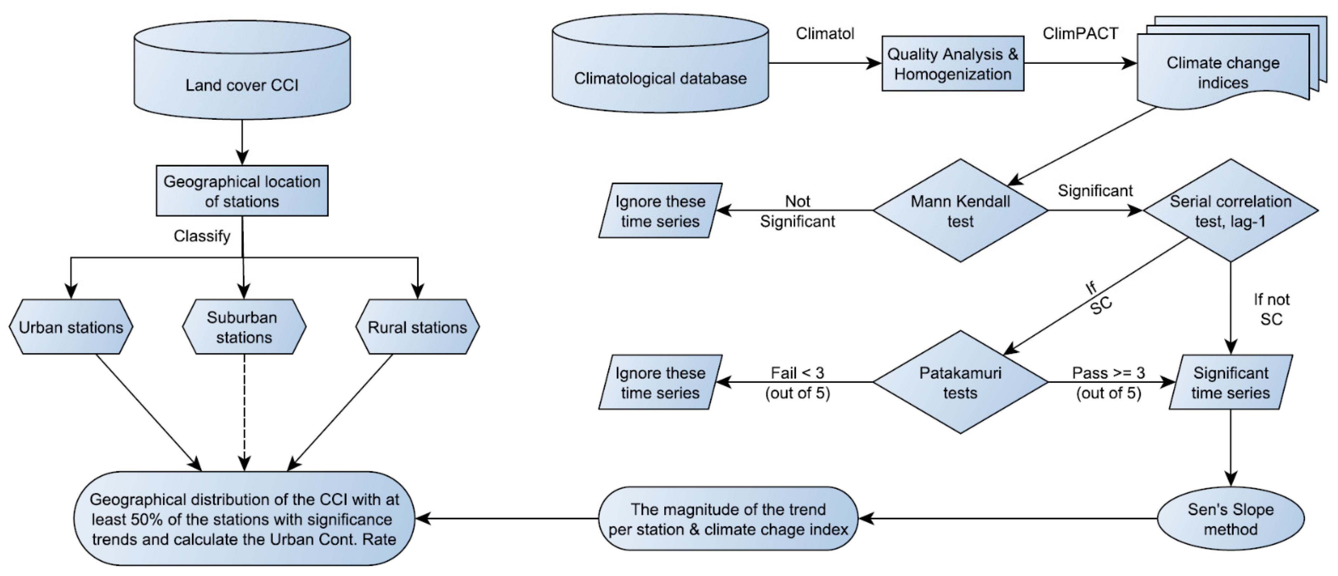
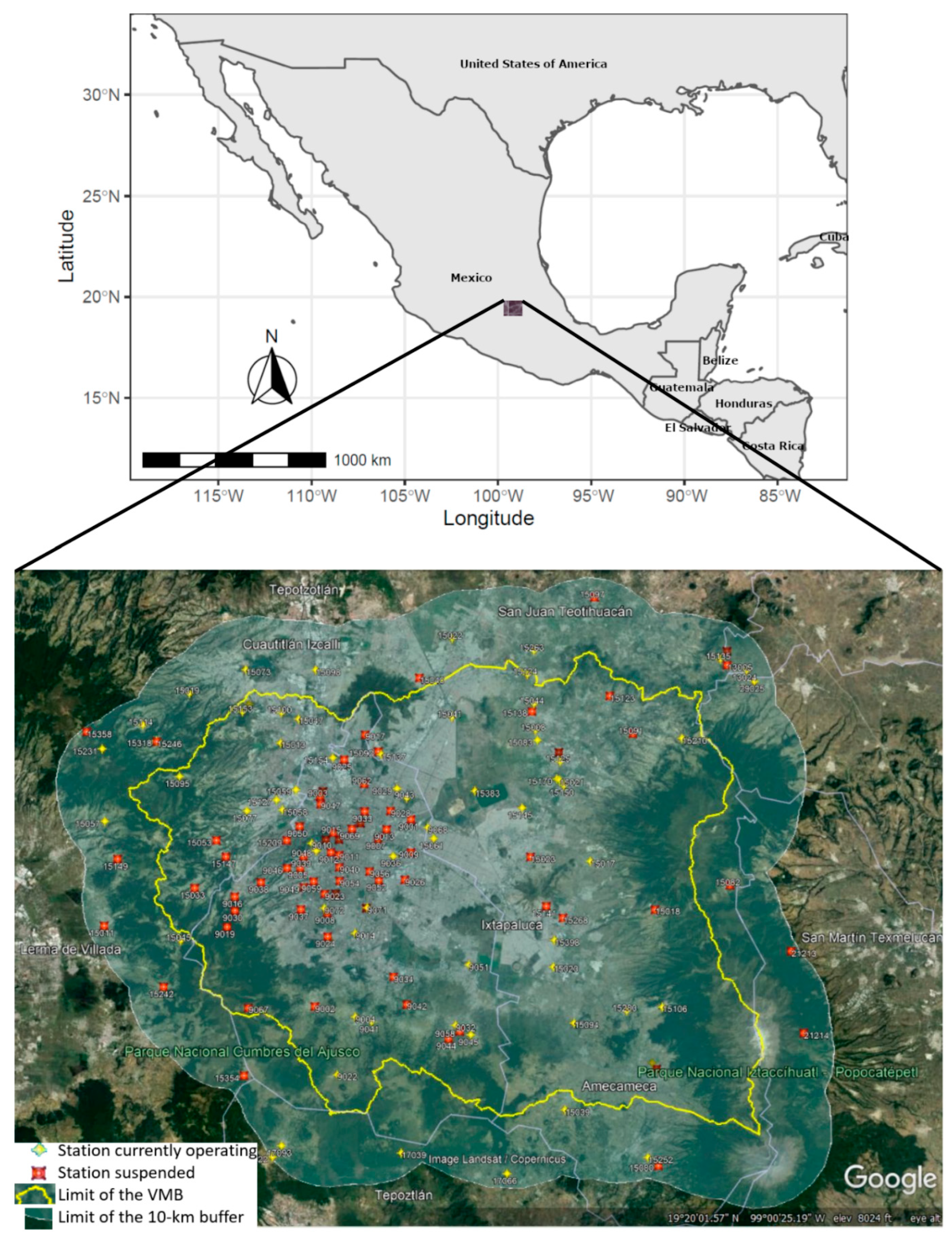
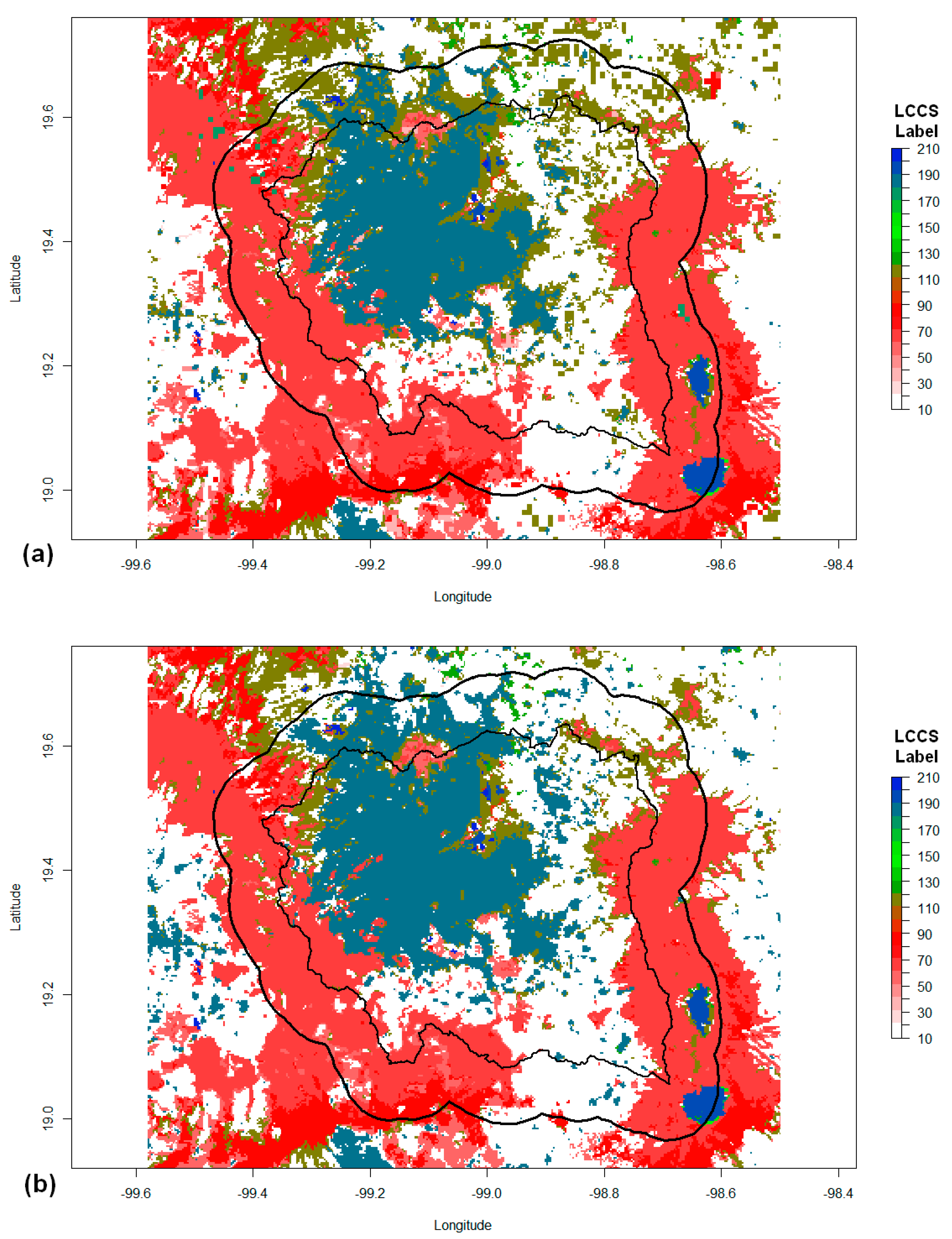
2.1. Study Domain, Data, and Station Classification

The VMB has a total area of 9738 km² and covers CDMX and different regions of the states of Mexico, Hidalgo, and Tlaxcala [43]. CDMX is one of the most densely populated regions in the world, with approximately 22 million people in an approximate area of 7850 km², and 97% of the population is concentrated in the basin [44,45]. CDMX has an average altitude of 2240 m above sea level (m a.s.l.) and is surrounded by mountains with peaks above 5000 m a.s.l. [45]. However, overpopulation is not the only problem currently affecting the area; it also faces one of the greatest pressures regarding water resources in the world [44]. Economically, approximately one-third of the entire Gross Domestic Product at the national level is generated in this region [44].

For the present study, information was collected from the daily climatic database of the National Meteorological Service of Mexico (SMN) for the variables of maximum temperature (TX), minimum temperature (TN), and precipitation (PR) in the period 1951–2010 [46]. Information was collected from 150 stations in the VMB area, including a 10 km buffer around the area for interpolation issues (Figure 2). For the process of data quality analysis and homogenization, only those stations that had at least 30% of the total data in the period 1951–2010 were chosen, in order to minimize the impact of information gaps. In this way, only 90 stations were obtained (

Table 1. Land-cover category in the years 1992 (LC_1992) and 2010 (LC_2010), geographical coordinates (Latitude and Longitude, in degrees), station identification number (Station ID), and station name of the 90 final climatological stations that were used for homogenization. The value 190 corresponds to urban land cover. The stations were classified as urban (u), suburban (s), and rural (r), next to the Station ID. See the other classification numbers in Table 2.

LC_1992	LC_2010	Latitude	Longitude	Station ID	Station Name
30	30	−99.2	19.217	9002 (r)	Ajusco
190	190	−99.19	19.469	9003 (u)	Aquiles Serdán 46
190	190	−99.117	19.417	9007 (u)	Cincel 42
190	190	−99.075	19.399	9009 (u)	Colonia Agrícola Oriental
120	70	−99.202	19.413	9010 (r)	Colonia América
190	190	−99.177	19.401	9012 (u)	Colonia Escandon
190	190	−99.106	19.428	9013 (u)	Colonia Moctezuma
190	190	−99.148	19.303	9014 (u)	Colonia Santa Ursula Coapa
190	190	−99.174	19.425	9015 (u)	Rodano 14 (CFE)
70	190	−99.3	19.35	9016 (s)	Cuajimalpa
70	70	−99.31	19.314	9019 (r)	Desierto de Los Leones
190	190	−99.182	19.297	9020 (u)	Desviación Alta al Pedregal
190	190	−99.186	19.475	9021 (u)	Egipto 7
11	11	−99.173	19.134	9022 (r)	El Guarda
190	190	−99.183	19.3	9024 (u)	Hacienda Peña Pobre
190	190	−99.158	19.513	9025 (u)	Hacienda La Patera
190	190	−99.083	19.367	9026 (u)	Morelos 77
190	190	−99.091	19.477	9029 (u)	Gran Canal Km. 06 + 250
70	70	−99.3	19.333	9030 (r)	La Venta Cuajimalpa
190	190	−99.022	19.191	9032 (u)	Milpa Alta
11	11	−99.1	19.25	9034 (r)	Moyoguarda
190	190	−99.217	19.333	9037 (u)	Presa Ansaldo
190	190	−99.267	19.367	9038 (u)	Presa Mixcoac
190	190	−99.213	19.397	9039 (u)	Presa Tacubaya
11	11	−99.129	19.197	9041 (r)	San Francisco Tlalnepantla
11	11	−99.083	19.217	9042 (r)	San Gregorio Atlapulco
70	70	−99.079	19.465	9043 (r)	San Juan de Aragón
120	190	−99.003	19.179	9045 (s)	Santa Ana Tlacotenco
190	190	−99.233	19.383	9046 (u)	Colonia Santa Fe
190	190	−99.189	19.46	9047 (u)	Colonia Tacuba
190	190	−99.196	19.404	9048 (u)	Tacubaya Central (Obs)
190	190	−99.213	19.36	9049 (u)	Tarango
190	190	−99.217	19.433	9050 (u)	Lomas de Chapultepec
190	190	−99.004	19.263	9051 (u)	Tláhuac
190	190	−99.053	19.429	9068 (u)	Puente La Llave
190	190	−99.172	19.351	9070 (u)	Campo Experimental Coyoacán
190	190	−99.132	19.334	9071 (u)	Colonia Educación
11	11	−98.642	19.61	13,024 (r)	Potrerito
11	11	−98.772	19.141	15,007 (r)	Amecameca de Juárez (Dge)
10	190	−98.913	19.544	15,008 (s)	Atenco
10	10	−99.468	19.318	15,011 (r)	Atarasquillo
190	190	−99.239	19.534	15,013 (u)	Calacoaya
190	190	−98.846	19.385	15,017 (u)	Coatepec de Los Olivos
11	190	−98.765	19.325	15,018 (s)	Colonia Manuel A. Camacho
120	120	−99.355	19.596	15,019 (r)	Colonia Vicente Guerrero
190	190	−98.896	19.258	15,020 (u)	Chalco -San Lucas-
11	11	−98.883	19.483	15,021 (r)	Chapingo (Obs)
11	11	−99.017	19.657	15,022 (r)	Chiconautla
120	120	−99.3	19.5	15,027 (r)	El Salitre
11	190	−99.351	19.361	15,033 (s)	Huixquilucan
11	11	−98.885	19.087	15,039 (r)	Juchitepec
190	190	−99.06	19.61	15,040 (u)	Gran Canal Km 02+120 Bombas
190	190	−99.019	19.562	15,041 (u)	Gran Canal Km 27+250
11	11	−98.914	19.576	15,044 (r)	La Grande
70	190	−99.369	19.299	15,045 (s)	La Marquesa
190	190	−99.216	19.563	15,047 (u)	Las Arboledas
11	11	−99.464	19.443	15,057 (r)	Mimiapan
190	190	−99.238	19.454	15,058 (u)	Molinito
190	190	−99.221	19.478	15,059 (u)	Molino Blanco
120	120	−99.282	19.623	15,073 (r)	Presa Guadalupe
120	120	−99.278	19.581	15,075 (r)	Presa Las Ruinas
190	190	−99.284	19.453	15,077 (u)	Presa Totolica
70	190	−98.67	19.353	15,082 (s)	Río Frío
190	190	−98.911	19.532	15,083 (u)	San Andrés
190	190	−99.114	19.522	15,092 (u)	San Juan Ixhuatepec
120	11	−98.871	19.19	15,094 (r)	San Luis Ameca
11	11	−99.368	19.495	15,095 (r)	San Luis Ayucan
190	190	−99.193	19.622	15,098 (u)	San Martín Obispo
120	11	−98.813	19.519	15,101 (r)	San Miguel Tlaixpan
190	190	−98.758	19.208	15,106 (u)	San Rafael
11	11	−99.414	19.558	15,114 (r)	Santiago Tlazala
11	11	−98.922	19.611	15,124 (r)	Tepexpan
190	190	−98.882	19.506	15,125 (u)	Texcoco (Dge)
190	190	−99.246	19.466	15127 (u)	Totolica San Bartolo
11	11	−98.675	19.624	15,135 (r)	Xochihuacan
11	190	−98.903	19.332	15,141 (s)	E.T.A. 032 Tlalpitzahuatl
190	190	−98.932	19.451	15,145 (u)	Plan Lago de Texcoco
190	190	−98.883	19.517	15,163 (u)	Texcoco (SMN)
11	11	−98.903	19.443	15,167 (r)	El Tejocote
11	190	−98.886	19.485	15,170 (s)	Chapingo (Dge)
190	190	−99.233	19.417	15,209 (u)	Presa San Joaquin
11	11	−98.727	19.53	15,210 (r)	San Juan Totolapan
70	70	−99.464	19.529	15,231 (r)	Presa Iturbide
120	190	−98.803	19.204	15,280 (s)	Tlalmanalco
70	60	−99.258	19.037	17,022 (r)	Tres Cumbres
90	90	−99.094	19.039	17,039 (r)	San Juan Tlacotenco
11	11	−98.65	19.6	29,006 (r)	Cuaula
11	11	−98.683	19.567	29,013 (r)	La Venta
11	11	−98.662	19.568	29,023 (r)	San Cristobal
11	11	−98.632	19.597	29,025 (r)	San Marcos Huaquilpan

) that meet this condition for the three variables: maximum and minimum temperature and precipitation.

For the classification of stations between urban, suburban, and rural, we used information from the Land Cover Climate Change (LC–CCI) of the European Space Agency [47]. The first phase of the LC–CCI generated a suite of products comprising 3 consistent global Land Cover (LC) products corresponding to the 1998–2002, 2003–2007 and 2008–2012 periods, representing seasonal dynamics of the land surface and Medium Resolution Imaging Spectrometer (MERIS) Surface Reflectance (SR) time series which served as input for generating the global land-cover maps [47].

Using tools from the LC–CCI website [47] (Figure 3, labels in

Table 2. Labels of the Land Cover Classification System (LCCS) [40] for the legend of Figure 3.

Label	Land Cover Classification System
10	Cropland, rainfed
20	Cropland, irrigated or post-flooding
30	Mosaic cropland (>50%)/natural vegetation (tree, shrub, herbaceous cover) (<50%)
40	Mosaic natural vegetation (tree, shrub, herbaceous cover) (>50%)/cropland (<50%)
50	Tree cover, broadleaved, evergreen, closed to open (>15%)
60	Tree cover, broadleaved, deciduous, closed to open (>15%)
70	Tree cover, needleleaved, evergreen, closed to open (>15%)
80	Tree cover, needleleaved, deciduous, closed to open (>15%)
90	Tree cover, mixed leaf type (broadleaved and needleleaved)
100	Mosaic tree and shrub (>50%)/herbaceous cover (<50%)
110	Mosaic herbaceous cover (>50%)/tree and shrub (<50%)
120	Shrubland
130	Grassland
140	Lichens and mosses
150	Sparse vegetation (tree, shrub, herbaceous cover) (<15%)
160	Tree cover, flooded, fresh or brackish water
170	Tree cover, flooded, saline water
180	Shrub or herbaceous cover, flooded, fresh/saline/brackish water
190	Urban areas
200	Bare areas
210	Water bodies

) and the coordinate information of the 90 selected climatic stations, the annual average land-cover values for the years 1992 and 2010 were obtained for each of the stations (Table 1). In this way, for the subsequent analysis, the stations were classified as: (i) urban, or those that had the value of 190 in the years 1992 and 2010; (ii) rural, those that had values different to 190 in the years 1992 and 2010; and iii) suburban, or those that had a value different from 190 for the year 1992, and 190 for 2020. No station recorded a value of 190 for the year 1992 plus a value different to 190 for the year 2010. The classification of each of the stations, according to the aforementioned parameters, is shown in Table 1 next to the identification number of the station with a (u) for urban ones, (s) for suburban ones, and (r) for rural ones. The total number of urban stations is 44, suburban 10, and rural 36.

2.2. Quality Control Analysis and Homogenization of Climate Data

One of the major problems of working with coarse climatological data is that they can be affected by non-climatic factors, whether they are errors in taking measurements, changes in instrumentation, or in the station’s environment. These alterations are known as inhomogeneities, and they mask the genuine changes in the climate, causing the study of climatic series to reach erroneous conclusions.

To solve this problem, we carried out the processes of quality control, homogenization, and in-filling of the missing data from the 90 climatic stations by applying the Climatol algorithm [48], version 3.1. Climatol uses the Standard Normal Homogeneity Test (SNHT) [49] to check the homogeneity of the climatic series, and the method of Paulhus and Kohler to fill-in daily series through averages of nearby stations [50]. Climatol has been used worldwide for the homogenization of climatic data [51,52,53].

2.3. Calculation of the Indices of the Daily Climate Extremes

The homogenized database was used as input to the ClimPACT2 software to calculate a set of 50 annual indices of daily climate extremes (

Table 3. Short name, long name, and definition of the 50 yearly CCI analyzed in the present study. The first 36 are temperature-related and last 14 are precipitation-related. The indices are defined in terms of maximum temperature (TX), minimum temperature (TN), mean temperature (TM), and precipitation (PR). Bold indicates indices also recommended by the ETCCDI.

Short Name	Long Name	Definition
FD	Frost Days	Number of days when TN < 0 °C
TNlt2	TN below 2 °C	Number of days when TN < 2 °C
TNltm2	TN below −2 °C	Number of days when TN < −2 °C
TNltm20	TN below −20 °C	Number of days when TN < −20 °C
ID	Ice Days	Number of days when TX < 0 °C
SU	Summer days	Number of days when TX > 25 °C
TR	Tropical nights	Number of days when TN > 20 °C
GSL	Growing Season Length	Annual number of days between the first occurrence of 6 consecutive days with TM > 5 °C and the first occurrence of 6 consecutive days with TM < 5 °C
TXx	Max TX	Warmest daily TX
TNn	Min TN	Coldest daily TN
TNx	Max TN	Warmest daily TN
TXn	Min TX	Coldest daily TX
DTR	Daily Temperature Range	Mean difference between daily TX and daily TN
WSDI	Warm spell duration indicator	Annual number of days contributing to events where 6 or more consecutive days experience TX > 90th percentile
WSDI5	WSDI-5	Annual number of days contributing to events where 5 or more consecutive days experience TX > 90th percentile
CSDI	Cold spell duration indicator	Annual number of days contributing to events where 6 or more consecutive days experience TN < 10th percentile
CSDI5	CSDI-5	Annual number of days contributing to events where 5 or more consecutive days experience TN < 10th percentile
TXgt50p	Fraction of days with above average temperature	Percentage of days where TX > 50th percentile
TX10p	Number of cool days	Percentage of days when TX < 10th percentile
TX90p	Number of hot days	Percentage of days when TX > 90th percentile
TN10p	Number of cold nights	Percentage of days when TN < 10th percentile
TN90p	Number of warm nights	Percentage of days when TN > 90th percentile
TMge5	TM of at least 5 °C	Number of days when TM ≥ 5 °C
TMlt5	TM below 5 °C	Number of days when TM < 5 °C
TMge10	TM of at least 10 °C	Number of days when TM ≥ 10 °C
TMlt10	TM below 10 °C	Number of days when TM < 10 °C
TXge30	TX of at least 30 °C	Number of days when TX ≥ 30 °C
TXge35	TX of at least 35 °C	Number of days when TX ≥ 35 °C
TX7TN7	7 consecutive hot days and nights	Annual count of 7 consecutive days where both TX > 95th percentile and TN > 95th percentile
TXb7TNb7	7 consecutive cold days and nights	Annual number of 7 consecutive days where both TX < 5th percentile and TN < 5th percentile
TMm	Mean TM	Mean daily mean temperature
TXm	Mean TX	Mean daily maximum temperature
TNm	Mean TN	Mean daily minimum temperature
HDDheat18	Annual sum of 18 − TM	A measure of the energy demand needed to heat a building
CDDcold18	Annual sum of TM − 18	A measure of the energy demand needed to cool a building
GDDgrow10	Annual sum of TM − 10	A measure of heat accumulation to predict plant and animaldevelopmental rates
CDD	Consecutive Dry Days	Maximum number of consecutive dry days (when PR < 1.0 mm)
CWD	Consecutive Wet Days	Maximum number of consecutive wet days (when PR ≥ 1.0 mm)
R10mm	Number of heavy rain days	Number of days when PR ≥ 10 mm
R20mm	Number of very heavy rain days	Number of days when PR ≥ 20 mm
R30mm	Number of extremely heavy rain days	Number of days when PR ≥ 30 mm
RX1day	Max 1-day PR	Maximum 1-day PR total
RX3day	Max 3-day PR	Maximum 3-day PR total
RX5day	Max 5-day PR	Maximum 5-day PR total
PRCPTOT	Annual total wet day PR	Sum of daily PR ≥ 1.0 mm
SDII	Daily PR intensity	Annual total PR divided by the number of wet days (when total PR ≥ 1.0 mm)
R95p	Total annual PR from heavy rain days	Annual sum of daily PR > 95th percentile
R99p	Total annual PR from very heavy rain days	Annual sum of daily PR > 99th percentile
R95pTOT	Contribution from very wet days	100 × r95p/PRCPTOT
R99pTOT	Contribution from extremely wet days	100 × r99p/PRCPTOT

). The first 36 indices listed in Table 3 are related to surface temperature (maximum, minimum and mean), and the last 14 to precipitation. ClimPACT2 is an R software tool that can read data for a single climate station as a text file, or for gridded data (e.g., from a climate model) as a netCDF files [54]. This software was developed by the Pacific Climate Impacts Consortium (PCIC).

The result is a time series for each of the 90 climate stations, with the annual mean value of each of the 50 daily climate extreme indices analyzed here.

2.4. Statistical Analysis of the Climate Change Indices Trends and Serial Correlation Test

Since the time series of the previous indices does not necessarily fulfill the assumption of normality, nonparametric methods (which work for all distributions) give better results. One of the most robust and widely used nonparametric methods in finding the statistical significance of trends is the Mann–Kendall test (sometimes called the M–K test) [55,56].

The M–K test is used to determine whether a time series has a monotonic upward or downward trend. Therefore, it is used here to detect the significant trends of every climate station time series of every extreme climate index. If the time series trends have no statistical significance, then they are simply ignored for the rest of the calculations. If the time series trends have statistical significance, then they are considered in the calculation procedure (Figure 1).

However, it is known that results are seriously affected when the time series are serially correlated [57]. For series that are serially correlated, the M–K trend test is not sufficient. To test the serial correlation in the data, the lag-1 serial correlation coefficients were calculated in the same way as in [57]. In this case, if the time series were serially correlated, then they were held for additional Patakamuri tests described in the next section. If the time series had no serial correlation, then they were kept as a completely statistically significant time series available to calculate the final trends, as described next (Figure 1).

2.5. Patakamuri Tests for Serially Correlated Data and Calculation of the Final Climate Indices Trends

Since there is no universal method for considering the serial correlation present in the time series, we followed here a method first applied by [57], in which five additional statistical tests were applied to the serially correlated time series. The tests carried out were:

• Prewhitening Mann–Kendall (PWMK) [58,59];
• Trend-free prewhitening Mann–Kendall (TFPWMK) [60];
• Bias correction applied to prewhitening (BCPW) [61];
• Variance correction approach suggested by Hamed and Ramachandra (MMKH) [62];
• Variance correction approach suggested by Yue and Wang (MMKY) [63].

These tests are extensively discussed in [57], so we will not repeat them here.

Following [57], we confirmed that if less than three tests (out of five) were favorable with at least 95% confidence, the serially correlated time series were taken as not statistically significant and simply ignored for the rest of the calculations. If at least three of the five tests mentioned above were favorable with at least 95% confidence, the time series with serial correlation was taken as statistically significant and kept together with the time series with no significant serial correlation to calculate the final trend of the time series (Figure 1).

The Sen’s slope method was selected to estimate the magnitude of the change trend of extreme climate indices (Figure 1). As a nonparametric method, Sen’s slope assumes a linear trend in the time series and then applies a linear model to calculate the slope of the trend [64,65]. The Sen’s slope method is also widely used for the analysis of hydrometeorological time series [66].

2.6. Calculation of the Average Climate Index Trend per Type of Station and Assessing the Effect of Urbanization on Extreme Climate Indices

Once Sen’s method was applied to estimate the magnitude of the change in the significant extreme climatic indices, the values of the slopes were grouped by each type of station (urban, rural, and suburban) to calculate an average value of the slope for each type of station and for each extreme climatic index. In the calculation of the averages, all the values of the slopes that were not statistically significant were obviously eliminated.

The values obtained were analyzed for each one of the climatic indices that had at least 50% of the significant values of the total number of stations (that is, at least 45 significant slope values).

To assess the effect of urbanization on extreme weather indices, we calculate what we call here the Urban Change Rate (UCR), which is simply,

$$UCR=\left(\frac{S_u-S_r}{S_r}\right)\times 100$$

(1)

where the values of S_u and S_r indicate the average change in the slope of the extreme climate indices for urban and rural stations, respectively. For simplicity, only the values between urban and rural stations are compared.

The results are shown below.

3. Results

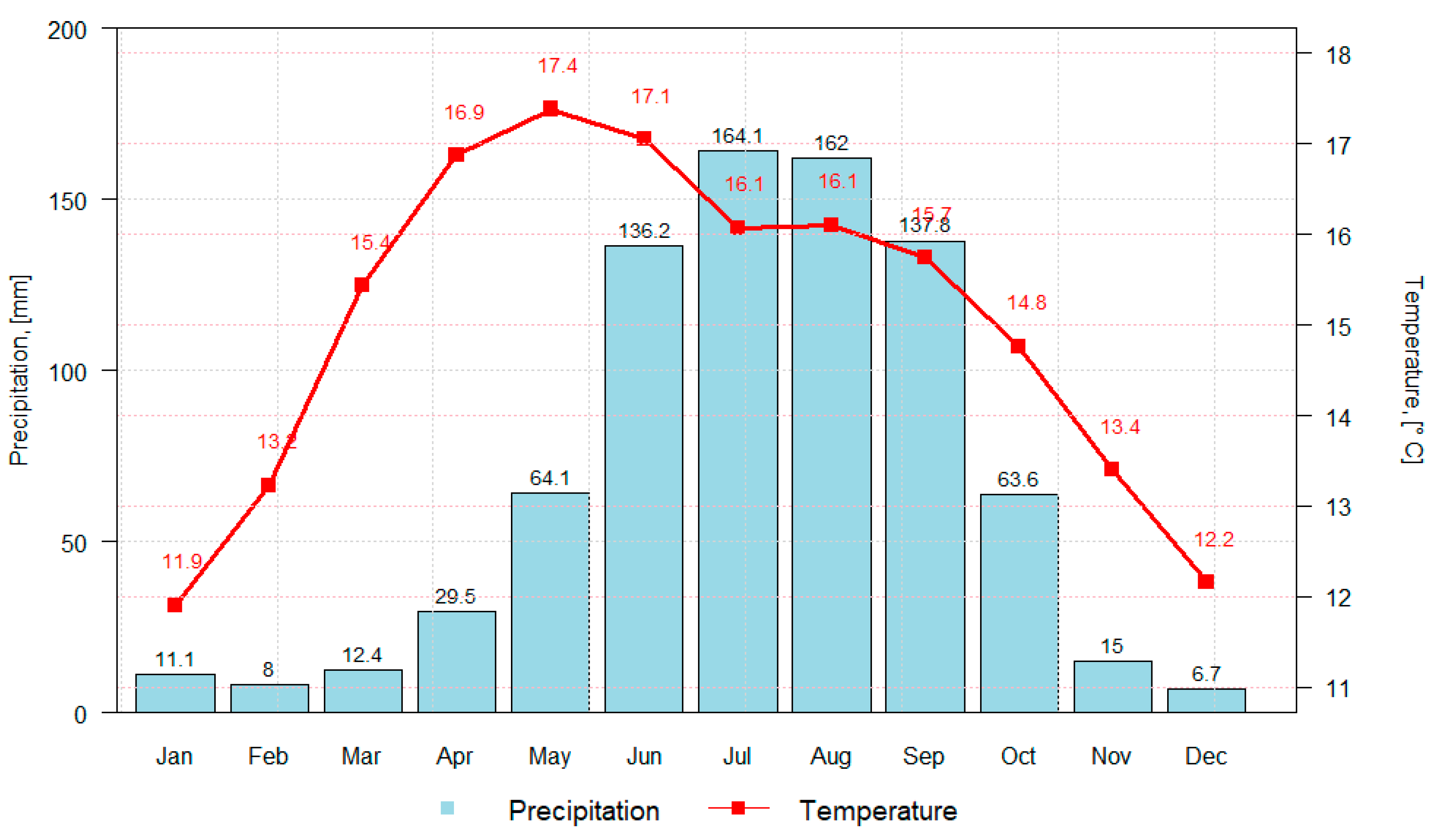
3.1. Mean Precipitation and Surface Temperature of the Homogenized Stations in the VMB

Some information on the data quality analysis and homogenization process is summarized in

Table 4. The mean of percentage of original data (MPOD), the total number of breakpoints, and outliers, are shown as a result of the homogenization process of maximum and minimum temperature, and precipitation. The numbers in parentheses show the number of stations that presented those breakpoints and outliers.

	MPOD	Breakpoints	Outliers
Maximum Temperature	36.24	44 (33)	7 (5)
Minimum Temperature	39.54	33 (28)	5 (4)
Precipitation	54.46	4 (4)	7 (5)

. It is notable (but not surprising) that the mean percentage of original data (MPOD) is significantly higher for precipitation (54.5%) than for maximum and minimum temperatures (36.2% and 39.5%, respectively). The above numbers are in accordance with the condition of using only climatic stations that had at least 30% of the total data in the period 1951–2010. In addition, it can be seen that the greatest number of breakpoints (simply defined as the non-climatic “jumps” or inconsistencies in the station) occurred for the maximum temperature, where 36.7% of the stations showed some breakpoints. The precipitation showed the least number of breakpoints, where only 3.7% of the stations showed some. For the outliers, the highest number was presented by the variables of maximum temperature and precipitation, and the lowest by the minimum temperature. The difference in the numbers and their corresponding number in parentheses in Table 4 means that in some cases, a given station showed more than one breakpoint and/or outlier. Details of these data are included as Supplementary Material (Tables S1–S6).

To explore the climatology of the VMB, a climograph is presented with the simple average of the data for precipitation and surface temperature of the 90 climatological stations that are within the limits of the study region (Figure 4). These values, however, should only be taken as a first rough approximation of the climatology of the basin. These values show us that the maximum average temperature occurs in April (17.4 °C) and the minimum is in January (11.9 °C). Meanwhile, the precipitation is of the monsoon type, with maximum precipitation in summer (July, 164.1 mm) and minimum precipitation in winter (December, 6.7 mm). Intra-summer drought is not presented in this information.

3.2. Statistical Analysis Results of the Climate Change Indices

From the homogenized time series of precipitation, maximum and minimum temperatures of each of the 90 weather stations were analyzed, the time series of the 50 climate change indices (Table 3) were obtained for each of the climate stations using the software ClimPACT2.

Using these CCI time series, and according to the methodology (Section 2.4 and Section 2.5), the trend detection tests (using the M–K test), serial correlation (calculating the lag–1) and the Patakamuri tests were used to discern the statistically significant series, despite them having serial correlation, and the results are shown in

Table 5. Statistics of the 50 CCI with the number of stations (out of 90) whose time series: (i) passed the M–K test for trend detection, (ii) were serially correlated, (iii) were rejected by the Patakamuri tests, and (iv) percentage of stations whose trend was statistically significant. The bold letters in the column of the climatic indices correspond to the ETCCDI indices, and the bold italics in the % column are those where at least 50% of the total were statistically significant.

Climate Temperature Index	M–K Test	Serially Correlated	Patakamuri Rejected	%	Climate Precipitation Index	M–K Test	Serially Correlated	Patakamuri Rejected	%
FD	83	71	9	82.2	CDD	5	1	0	5.6
TNlt2	16	15	0	17.8	CWD	50	36	10	44.4
TNltm2	49	41	8	45.6	R10mm	27	6	3	26.7
TNltm20	0	0	0	0.0	R20mm	41	25	5	40.0
ID	0	0	0	0.0	R30mm	37	14	5	35.6
SU	65	51	7	64.4	RX1day	32	17	7	27.8
TR	0	0	0	0.0	RX3day	18	3	0	20.0
GSL	3	3	0	3.3	RX5day	19	3	0	21.1
TXx	45	22	7	42.2	PRCPTOT	34	4	0	37.8
TNn	78	76	4	82.2	SDII	53	43	13	44.4
TNx	48	40	14	37.8	R95p	36	23	7	32.2
TXn	50	31	10	44.4	R99p	30	12	3	30.0
DTR	41	38	15	28.9	R95pTOT	33	25	6	30.0
WSDI	65	42	11	60.0	R99pTOT	26	12	4	24.4
WSDI5	67	48	4	70.0
CSDI	76	42	14	68.9
CSDI5	83	65	8	83.3
TXgt50p	81	80	15	73.3
TX10p	70	61	10	66.7
TX90p	68	67	3	72.2
TN10p	79	76	8	78.9
TN90p	48	46	13	38.9
TMge5	19	7	1	20.0
TMlt5	25	3	0	27.8
TMge10	40	37	2	42.2
TMlt10	40	37	3	41.1
TXge30	8	3	1	7.8
TXge35	0	0	0	0.0
TX7TN7	0	0	0	0.0
TXb7TNb7	0	0	0	0.0
TMm	83	83	7	84.4
TXm	26	26	2	26.7
TNm	75	75	12	70.0
HDDheat18	84	84	5	87.8
CDDcold18	15	9	1	15.6
GDDgrow10	80	80	6	82.2

. In addition, the percentage of stations (of the total of 90) whose trends were statistically significant for each CCI is also shown, highlighting in bold the values with a percentage of at least 50%.

The results show that the indices related to temperature that had the highest percentage of stations that passed the M–K test were HDDheat18, with 93.3% and FD, CSDI5 and TMm, with 92.2% each (all these indices related to temperature). The minimum percentages occurred for the TNltm20, ID, TR, TXge35, TX7TN7 and TXb7TNb7 indices, at 0%. For the indices related to precipitation, the highest percentage was for SDII (58.9%) and CWD (55.6%), while the minimum was for CDD (5.6%).

The results for serially correlated series (with the lag-1 test) show that they were quite common. Remembering that these tests were only applied to the tests that passed the M–K test, it can be seen in Table 5 that for the indices related to temperature, 100% of the stations were serially correlated for the indices of HDDheat18, TMm, GDDgrow10, TNm, and TXm. For the indices related to precipitation, the highest percentage of serially correlated series was found by SDII, with 81.1%, and the lowest percentage was for PRCPTOT, with only 11.8%.

For the Patakamuri tests, the highest percentage of rejections of the total series that were serially correlated for the indices related to temperature was for the DTR (39.5%), and for the precipitation indices it was for R10mm (50%).

Finally, the indices related to temperature with the highest percentages of stations whose trends were statistically significant were HDDheat18 (87.7%) and TMm (84.4%). For the indices related to precipitation, these were CWD and SDII, with 44.4% each. In the present work, further analysis was carried out with only the indices that showed statistically significant trends in at least 50% of the stations (shown in

Table 6. Arithmetic average of the trends in the climatological stations classified as urban, suburban, and rural, that were statistically significant for the indices: FD (days/year), SU (days/year), TNn (°C/year), WSDI (days/year), WSDI5 (days/year), CSDI (days/year), CSDI5 (days/year), TXgt50p (%/year), TX10p (%/year), TX90p (%/year), TN10p (%/year), TMm (°C/year), TNm (°C/year), HDDheat18 (degree days/year), and GDDgrow10 (degree days/year). The indices in bold belong to the ETCCDI list. The Urban Change Rate (UCR) calculated with the slopes of the urban and rural stations is also shown.

Climate Index	Urban	Suburban	Rural	Urban Change Rate (%)
FD	−0.289	−0.333	−0.511	−43.41
SU	1.040	0.605	0.640	62.55
TNn	0.087	0.060	0.085	2.52
WSDI	0.010	0.006	0.055	−82.62
WSDI5	0.118	0.130	0.134	−11.63
CSDI	−0.094	−0.045	−0.069	35.70
CSDI5	−0.218	−0.202	−0.178	22.12
TXgt50p	0.409	0.427	0.346	18.32
TX10p	−0.152	−0.146	−0.157	−2.72
TX90p	0.191	0.206	0.178	7.35
TN10p	−0.236	−0.186	−0.190	24.01
TMm	0.023	0.022	0.022	7.75
TNm	0.031	0.026	0.023	32.89
HDDheat18	−6.522	−6.891	−7.233	−9.84
GDDgrow10	8.250	7.376	6.843	20.56

). None of the indices related to precipitation met this requirement.

The last part of the analysis of this work shows the results of the 15 indices whose number of stations with statistically significant trends was at least 50% of the total (Table 6). Table 6 makes a simple comparison between the arithmetic averages of the statistically significant trends for the stations classified as urban, suburban, and rural, in each of these 15 indices. In addition, the urban change ratio described in the methodology (Section 2.6) is calculated.

As a first approximation, one would expect the average values of the trends for the suburban stations to be “in between” the values for the urban and rural stations. However, according to the results in Table 6, this only happens for the indices FD, WSDI5, CSDI5, TMm, TNm, HDDheat18, and GDDgrow10. Part of the explanation for this discrepancy could be due to the sizeable difference between the number of suburban stations (10) and the number of urban (44) and rural stations (36). The most contrasting values in the average of the statistically significant trends of the urban stations with the rural ones are somehow expressed by the magnitude of the value of the urban rate of change. It is observed that the highest positive value of the UCR when the seasonal trends are positive occurs for SU (62.55%), which implies that urbanization contributes to a significant increase in the trend. The highest positive value of UCR when the trends are negative is for CSDI (35.70%), which implies that urbanization favors a further decrease in the trend. The highest negative value of UCR when trends are positive is for WSDI (−82.62%), which implies a decrease in trend associated with urbanization. Finally, the most negative value of UCR when the trends are negative is for FD (−43.41%), which implies an increase in the trend related to urbanization.

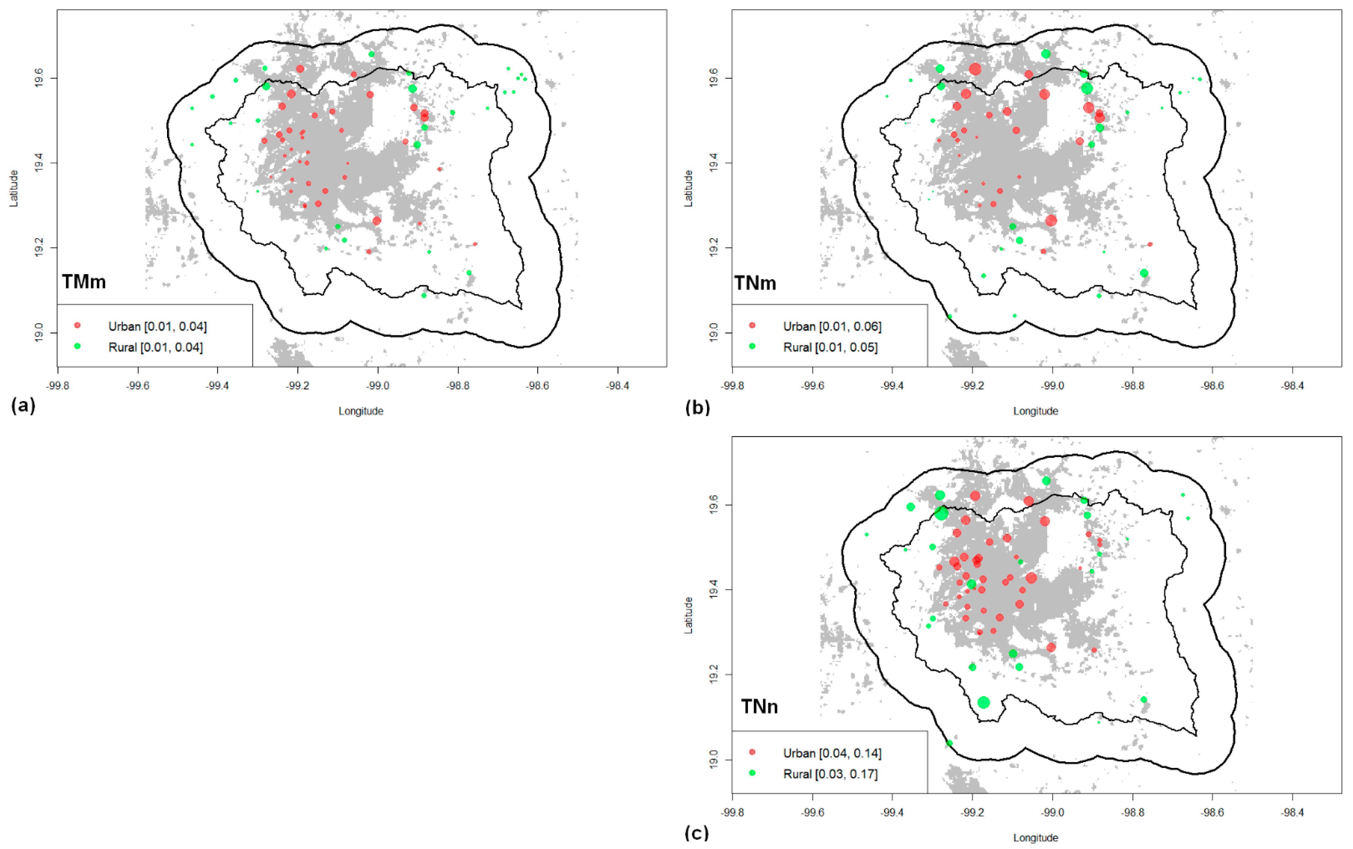
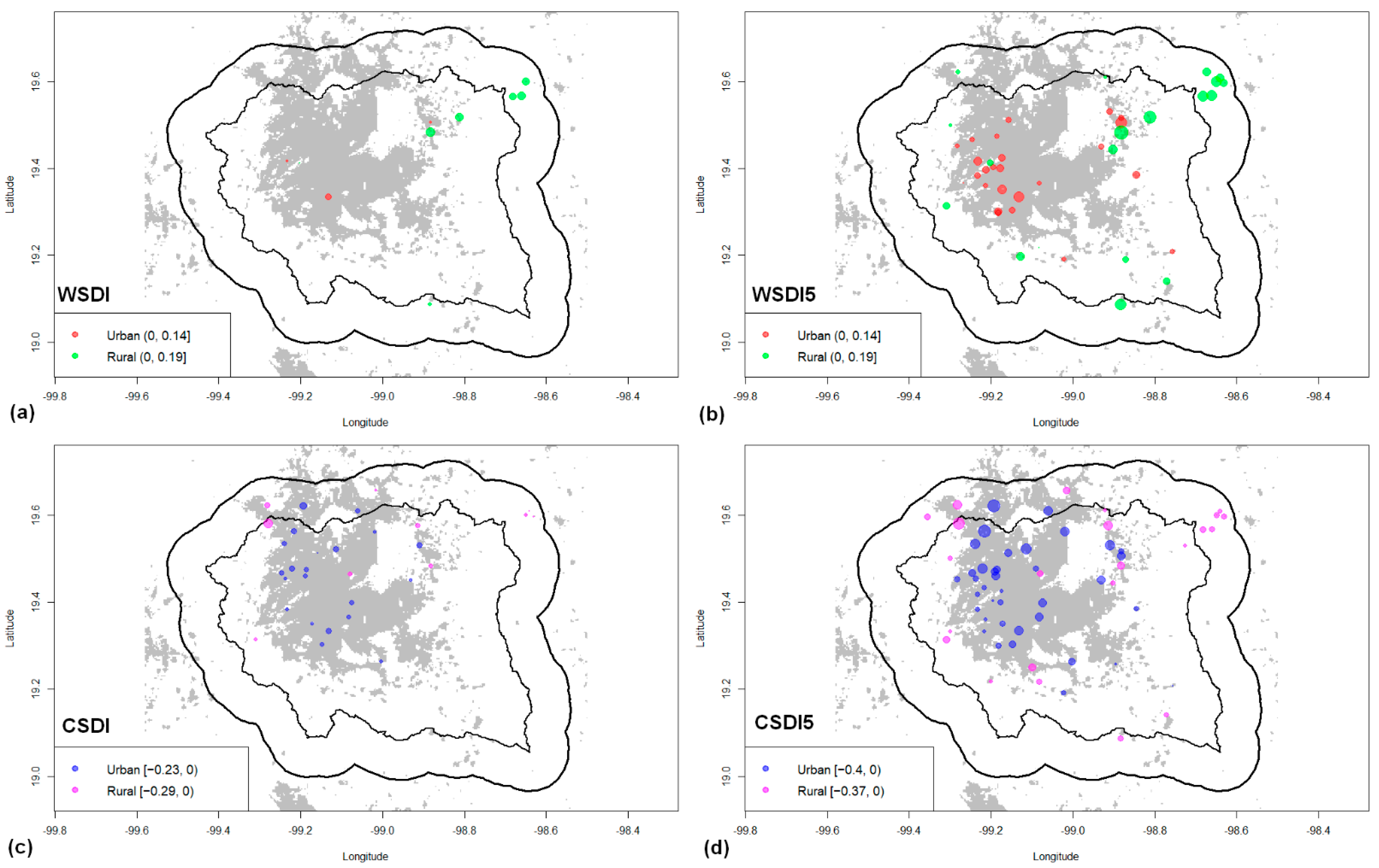
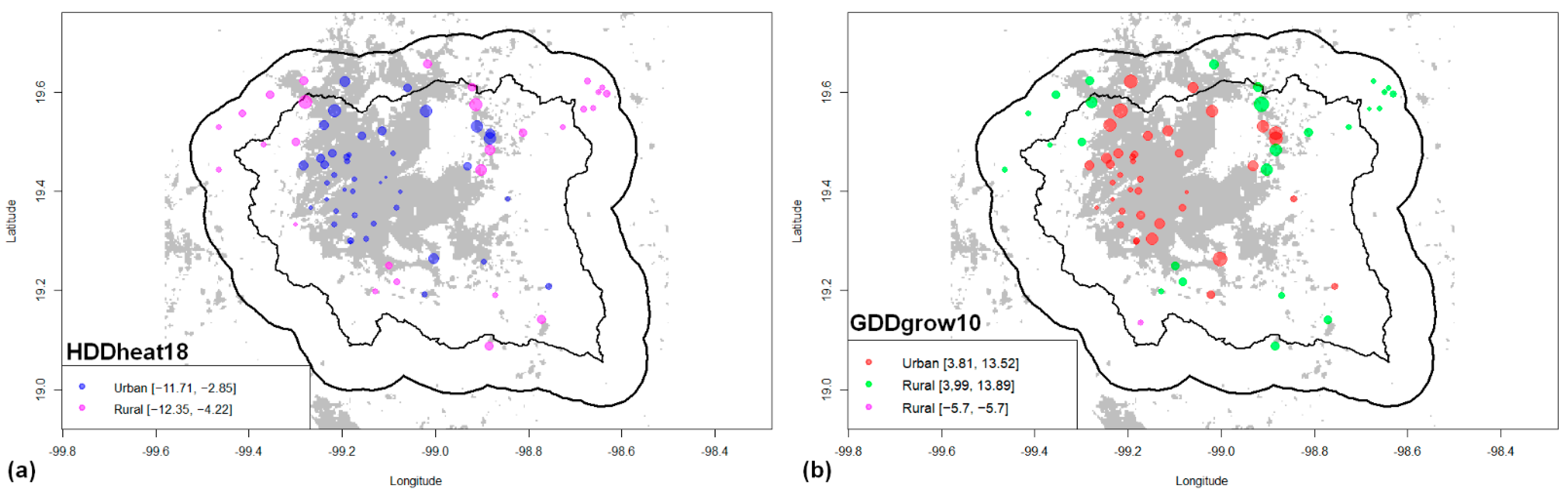
3.3. Geographic Distribution of Statistically Significant Urban and Rural Station Trends for Some CCI

The geographic distribution of the urban and rural stations that had statistically significant trends for each of the 15 CCI shown in Table 6 is presented below.

The results for FD (Figure 5a) show only negative trends (days/year) for all stations that showed statistically significant trends. The most negative trends in the urban stations are towards the northeast and center of CDMX (large gray spot in the figure). For the rural stations, the most negative trends (despite the lesser magnitude than the two largest urban ones) are to the southwest of the VMB and to the north in rural areas very close to the urban area.

In contrast, for SU the statistically significant trend values were all positive for all stations (Figure 5b). The maximum value of approximately 2.5 days/year occurs in the City of Texcoco (gray spot to the right of CDMX). For the rural area, the maximum trend is 1.77 days/year in a station close to the south of the maximum in the urban area. It is also possible to observe several values of significant magnitude in the center and southwest of CDMX.

For TMm, the statistically significant trend values were positive for all stations (Figure 6a). However, the magnitudes of the maximum values for both types of stations were relatively small, at around 0.04 °C/year. Such maximum values were presented to the northwest of CDMX and around the City of Texcoco for both types of stations.

The results for TNm are shown in Figure 6b. The trend values were all positive again for all stations, although slightly higher in the maximum values (0.06 °C/year). Such maximum values were presented mainly to the north of the CDMX and the VMB.

The results for TNn are shown in Figure 6c. Here, the values of the statistically significant trends are also positive but considerably higher in magnitude (compared to TMm and TNm) for all stations (0.17 °C/year for rural stations and 0.14 °C/year for urban stations). Again, the maximum values for both types of stations occurred northeast of the VMB and CDMX (besides the maximum value for the rural station southwest of the VMB), but there are also several values of average magnitude in the center of CDMX.

Figure 7 shows the results for various extreme climate indices, such as TX90p, TXgt50p, TX10p, and TN10p. For TX90p (Figure 7a), positive and negative trend values are presented (although only for rural areas in the latter case). Positive values prevail and maximum values are presented for urban stations with trends of up to 0.37 °C/year. Maximum values prevail in the southern zone of CDMX for the urban zone. For rural stations, the maximum values (up to 0.28 °C/year) occur in the eastern zone (north and south) of the VMB. Additionally, the number of rural stations that presented significant increases in this index is notable. The few negative values for rural stations occur to the southwest of the VMB.

For TXgt50p, positive and negative trends reappear in the VMB, with the positive ones prevailing again (Figure 7b). It is notable that the highest magnitude value is a rural station to the southwest of the VMB, with a value of −0.91 °C/year. The positive values of the rural stations are found mainly to the south of Texcoco (maximum value of 0.73 °C/year), and other important positive values lie to the northwest and southwest of the VMB. The positive maximum of the urban stations is found in Texcoco (0.68 °C/year), and other important positive trend values are found, especially in the western part of CDMX.

For TX10p, only negative trends are presented for all stations (Figure 7c). The most significant values occur in the west–central part of CDMX and in the northwest of the VMB, where the highest magnitude values were close to −0.25 °C/year.

For TN10p, again only negative trends were found (Figure 7d). The trend value with the largest negative magnitude (−0.25 °C/year) occurred in an urban station north of CDMX, and important values were found in that region. For rural stations, the maximum value occurred south of CDMX, and other important values were found north of Texcoco and northwest of CDMX.

The results for WSDI, WSDI5, CSDI, and CSDI5 are presented in Figure 8. For the analysis of results, the maximum value in terms of magnitude of the trends of the WSDI and WSDI5 pairs, and of CSDI and CSDI5, was set. For WSDI (Figure 8a) and WSDI5 (Figure 8b), we observe that there is good consistency according to the definition of the indices, since with WSDI (annual number of days contributing to events where 6 or more consecutive days experience TX > 90th percentile), the number of significant stations and magnitude of positive trends is considerably lower than for WSDI5 (same definition as WSDI but for 5 or more consecutive days). This is to be expected, as the condition is obviously more likely to occur at the last index. The magnitude of change in a single-day difference in the condition of the indices is surprising. The stations with trends of significant magnitude are found mainly to the northeast of the VMB (rural) and to the west, center, and south of CDMX.

A similar case, but with negative trends, is presented in the comparison between CSDI (Figure 8c) and CSDI5 (Figure 8d). Again, there is a high consistency between the location of stations, with significant negative trends and an always lower magnitude of CSDI compared to CSDI5. Here, the trends of greater magnitude for both indices are found mainly north of CDMX for urban stations and northwest of the VMB for rural stations very close to the urban area.

Finally, the results for the HDDheat18 (Figure 9a) and GDDgrow10 (Figure 9b) indices are shown. A strong spatial correlation between both indices is shown, with the difference that HDDheat18 presents negative trends and GDDgrow10 positive trends (except for one season). Both indices show that their trends of greatest magnitude are found in the northern zone of CDMX and Texcoco and in rural stations very close to these same urban zones. With GDDgrow10, the only station with negative trends occurs to the southwest of the VMB.

4. Discussion

4.1. Analysis of the Climate Change Indices

The analysis of the behavior of the CCI for a region is important for the design of potential protocols for civil protection against extreme events, especially in a megalopolis such as the Metropolitan Zone of Mexico City.

According to the results shown in Table 6 for the three types of stations in the Valley of Mexico basin, the summer days (SU), the mean daily mean temperature (TMm), the mean daily minimum temperature (TNm), the coldest daily minimum temperature (TNn), the fraction of days with above average temperature (TXgt50p), the amount of hot days (TX90p), and the warm spell duration indicator (WSDI) all increased during the 60-year study period (1951–2010). On the other hand, the frost days (FD), the number of cool days (TX10p), the number of cold nights (TN10p), and the cold spell duration indicator (CSDI), all decreased during the same period. The above means that the mean temperature and some of the extreme maximum temperature indices increased, but some of the extreme minimum temperature indices decreased for all the VMB.

As we show later, these results are in strong agreement with the trends obtained at a global level by [8], and at a regional level for many USA cities reported by [28]. The frost index, FD, in the present work, finds negative trends for all the stations that had significant trends in the CDMX and in the VMB (Figure 5a). This result is in perfect agreement with the global negative trend published by [8] with the GHCNDEX and HadGHCND databases for the period 1951–2011. It also agrees with the IPCC report [67], where one of the impacts of anthropogenic climate change is expected to be a decrease in extreme cold day events. One of the first studies to prove that type of trend for a given region was that of [68] for the USA. In addition, it is found that for rural areas, the values of this index decrease more quickly than in urban areas, which could be due to local effects of the area, such as soil degradation [69]. However, this result contrasts with what was found by [30], given that they find a negative trend for station 9014 in the central west of CDMX, no trend for station 9029 in the north of CDMX, and a negative trend for station 9032 in the south of CDMX. The difference between these results may be due to the difference in the study period compared to [30], since they used only 1980–2010. As we know, trends over a shorter period of time can sometimes significatively differ (even in sign) from the trends over a larger period.

For the summer days, SU, the present work finds positive, significant trends for all the stations of the CDMX (and the VMB). This result agrees with the positive global trend found by [8] for practically the same study period. In contrast, the authors in [30] find significant negative trends for the three stations in CDMX.

The positive trends found for TMm (Figure 6a) and TNm (Figure 6b) are of the order of 10⁻¹ °C/decade, which are similar to those those found by the authors in [70], who report similar warming in much of the Mesoamerican region. This is also in agreement with the positive annual trends for TX, TN and TM (although not statistically significant at 95%) found by [71] for CDMX.

Again, for the TNn index (Figure 6c) the results found in this study differ from those found by [30], given that they found only a positive trend for station 9014 in the central–west of CDMX, no trend for station 9029 in the north of CDMX, and a positive trend for station 9032 in the south of CDMX. The present work, as described above, we only found positive trends for all stations, with a significant trend in CDMX.

Regarding the number of hot days (TX90p Figure 7a), the positive trends found are consistent with the global trends reported by [8], and with what was found by [28], although in the latter case, they found increases in the number of warm days, but not nearly as many as in the number of warm nights. Regarding the comparison of these results with those found by [30], they are completely different. They find negative trends for the three CDMX stations, and the present work clearly finds statistically significant positive trends for these urban stations.

The negative trends in the number of cold days (TX10p, Figure 7c) reported here for CDMX and VMB are clearly consistent with the negative trends reported globally by [8]. However, in the work of [28], although they find a higher frequency in negative trends, there are some urban areas with positive trends. The comparison of results of this same index with those found by [30] are again completely different, since they find positive trends for the three stations in CDMX and in this work we find negative trends for all stations, with a significant trend in CDMX.

The negative trends found in this work for cold nights (TN10p, Figure 7d) are consistent with the global trend reported by [8] and with the results of [28], where the latter finds a statistically significant decrease in urban areas, with a median decline of 7.6% per decade for those areas with significant downward trends. On the other hand, the trends found in this work for CDMX differ from those found by [30]. They find positive trends for stations 9029 and 9032 north and south of CDMX, respectively, and a positive trend for 9014 in the center–west of CDMX. However, the present work only finds significant negative trends for all stations in CDMX and VMB.

Regarding the two warm spell duration indicator indices (WSDI and WSDI5, Figure 8a,b, respectively), the positive trends found for CDMX and VMB agree with the global trends reported by [8] and with those reported by [28] for urban areas of the USA. However, even though our results for WSDI coincide with the more frequent signal of the trends found by [28], in general, the differences appear to be mostly attributable to regional changes in climate, rather than to local effects of urbanization. On the other hand, the negative trends found here for the two cold spell duration indicators (CSDI and CSDI5, Figure 8c,d, respectively) agree with the global negative trends reported by [8] and with most of those reported by [28]. We note that there is a significant spatial correlation between CSDI and TN10 (Figure 7d). The fact that CSDI (and CSDI5) is decreasing faster for urban compared to rural areas (as supported by this study) is explained in previous research [72], which discusses that a UHI not only has negative effects (as a lot of heat during summer), but also “positive” effects, as cities can serve as warm shields during cold waves.

The negative trends found for HDDheat18 In the VMB were consistent with the result of [28] for this index in the USA, where about 50% of the urban areas had significant declines, while none had a significant increase in HDD.

The positive trends observed, both in urban and rural areas, in several of the temperature-related indices, may be an indicative of a global warming effect. This is strengthened by all the indices analyzed here having a strong correspondence with the signal of global trends [67].

In addition, it was observed that in urban areas where the heat island effect is detected—the UHI for the Valley of Mexico area—we have used the average of the TNm index for the urban area (8.52 °C) and the rural area (6.15 °C) and we have obtained the difference between them, at a value of (2.37 °C). This value reveals the heating due to the heat island effect in the urban area. If we translate it to change per decade, we have 0.39 (°C/decade). This is a rate of warming between the range (0.57 and 0.37 °C/decade) reported by [34]. Another study [73] reports a UHI of 1.94 °C; however, they cover a larger area than the VMB present in this study.

Changes in precipitation extremes are spatially less consistent compared to the dominant warming observed in the temperature indices over the last 60 years, and are also mostly less significant [8]. The results found in this study are also in agreement with the global values found by [8]. As [28] explains, the smaller number of statistically significant trends compared to temperature-related indices may well be a result of higher natural variability in precipitation extremes related to temperature.

It is known that temperature increases can cause discomfort, economical loss, migration, and increased mortality rates on a global level [74]. Our results indicate changes in climate in the VMB during the 1951–2010 period that have potentially profound implications for urban residential heating and cooling, and other ecological, social and health issues. However, additional work will be needed to quantify these impacts, and to estimate associated uncertainties in the CDMX. Nevertheless, several studies have already analyzed those impacts at global and regional levels. For instance, as [75] points out, in the future, climate change, combined with population aging and declining public spending on health and social care, may aggravate inequalities in health outcomes related to climate change. According to [76], the urban climate often differs from the surrounding rural countryside as it is generally more polluted, warmer, rainier and less windy. This indicates that the effect of climate change with the predicted increase in temperature and more extreme weather events will be experienced to a greater extent in urban areas compared to the surrounding landscape [77]. The changing climate might also exaggerate the negative effects of urbanization already experienced, such as increased urban temperatures and flooding [78].

4.2. Some Recommendations to Reduce Current and Future Impacts

The present study provides results on the behavior of climatic indices in the VMB, which includes CDMX, showing the effects of both climate change and heat islands. A previous study was carried out by the Economic Commission for Latin America and the Caribbean [79], which reports that the heat island phenomenon in cities in Latin America is perceived in 78 cities in 13 countries, and among them they located the CDMX. One of the effects of the heat island is perceived in the human population, who suffer stress or reduced comfort when carrying out their activities, including labor productivity (Seppanen et al. 2006). Other effects of the increase in temperature are heat strokes that also affect health, including some cases of mortality [37]. There are also impacts on urban services, such as the growing demand for energy and water [79]. The water balance is sensitive to changes in climate and basin conditions, the change in land use (e.g., paving) affects the infiltration of precipitation and can increase runoff [80]. The authors in [42] find that land use change in the Mexico City basin has a significant impact on surface wind circulation.

The recommendations made to reduce heat island effects are [81]:

• Increase green areas, especially near homes, to promote cooling and reduce energy demand and costs, in addition to improving air quality. Examples of this can be planting trees and/or transforming roofs into ecological areas such as roof gardens.
• Build cold roofs, which are reflective, and are characterized according to their slope.
• Increase the use of more efficient electronic devices and equipment; this helps to reduce energy consumption, and in turn, its losses.

CDMX has developed a local climate action strategy, which includes the heat island effect, and adds to the effects of other hydrometeorological phenomena influenced by climate change. This strategy suggests an inclusive and transformative climate policy, with actions that have a gender, social inclusion and human rights perspectives, in addition to generating green jobs, contemplating revegetation programs for the city and the countryside, improving air quality and promoting climate culture, among others [82].

5. Conclusions

The main contribution of the present study, compared to others in the CDMX region, is the analysis of 50 climate change indices over a 60-year period (1951–2010), working with a set of 90 quality-controlled and homogenized data series.

The positive trends found for the CDMX (and in general in the VMB) in SU, TMm, TNm, TNn, TX90p, and WSDI, as well as the negative ones in FD, TX10p, TN10p, CSDI, and HDDheat18, and the strong correspondence of the trends obtained at global [8] and regional levels [28], certainly point to an influence of anthropogenic global warming on this region, rather than to local effects of urbanization. Similar results have been found in other studies [29,83].

The apparent discrepancy between the results found in the present study and those reported by [30] for the trends in FD, SU, TNn, TX90p, TX10p, and TN10p could be due to the difference in the study period, given that [30] used 1980–2010 and the present study used 1951–2010. Some additional analysis will be needed to probe whether this is the case.

It is very likely that significant changes in the UCR (Table 6), both negative (as with WSDI, −82.62% and FD, −43.41%) and positive (SU, 62.55% and CSDI, 35.70%), could be due to local effects such as the difference in land cover that occurs in urban stations compared to rural stations. As we know, this type of difference in land cover results in differences in the surface albedo, which implies a modification of the surface radiative balance near such stations, resulting in effects such as the well-known heat island or changes in extreme weather indices, such as in the present case.

Unfortunately, the CCI related to precipitation turned out to have low percentages of stations with statistically significant trends, and could not be used to infer anything about these important indices for a megalopolis that has a severe problem regarding the availability of water resources for its population.

References

1. Arguez, A.; Hurley, S.; Inamdar, A.; Mahoney, L.; Sanchez-Lugo, A.; Yang, L. Should we expect each year in the next decade (2019–28) to be ranked among the top 10 warmest years globally? Bull. Am. Meteorol. Soc. 2020, 101, E655–E663. [Google Scholar] [CrossRef] [Green Version]
2. Easterling, D.R.; Meehl, G.A.; Parmesan, C.; Changnon, S.A.; Karl, T.R.; Mearns, L.O. Climate Extremes: Observations, Modeling, and Impacts. Science 2000, 289, 2068–2074. [Google Scholar] [CrossRef] [PubMed] [Green Version]
3. IPCC. Climate Change 2007: Synthesis Report. Contribution of Working Groups I, II and III to the Fourth Assessment Report of the Intergovernmental Panel on Climate Change; Core Writing Team, Pachauri, R.K., Reisinger, A., Eds.; IPCC: Geneva, Switzerland, 2007; p. 104. [Google Scholar]
4. IPCC. Climate Change 2014: Synthesis Report. Contribution of Working Groups I, II and III to the Fifth Assessment Report of the Intergovernmental Panel on Climate Change; Core Writing Team, Pachauri, R.K., Meyer, L.A., Eds.; IPCC: Geneva, Switzerland, 2014; p. 151. [Google Scholar]
5. IPCC. Climate Change 2021: The Physical Science Basis. Contribution of Working Group I to the Sixth Assessment Report of the Intergovernmental Panel on Climate Change; Masson-Delmotte, V., Zhai, A.P., Pirani, S.L., Connors, C., Péan, S., Berger, N., Caud, Y., Chen, L., Goldfarb, M.I., Gomis, M., et al., Eds.; Cambridge University Press: Cambridge, UK, 2021; in press. [Google Scholar]
6. Expert Team on Climate Information for Decision-Making. Available online: https://community.wmo.int/governance/commission-membership/commission-weather-climate-water-and-related-environmental-service-applications-sercom/commission-services-officers/sercom-management-group/standing-committee-climate-services/expert-team-climate-information-decision (accessed on 11 April 2022).
7. Peterson, T.C.; Manton, M.J. Monitoring Changes in Climate Extremes: A Tale of International Collaboration. Bull. Am. Meteorol. Soc. 2008, 89, 1266–1271. Available online: http://www.jstor.org/stable/26220889 (accessed on 11 April 2022). [CrossRef]
8. Donat, M.G.; Alexander, L.V.; Yang, H.; Durre, I.; Vose, R.; Caesar, J. Global land-based datasets for monitoring climatic extremes. Bull. Am. Meteorol. Soc. 2013, 94, 997–1006. [Google Scholar] [CrossRef] [Green Version]
9. Sui, Y.; Lang, X.; Jiang, D. Projected signals in climate extremes over China associated with a 2 °C global warming under two RCP scenarios. Int. J. Climatol. 2018, 38, e678–e697. [Google Scholar] [CrossRef]
10. Panda, D.K.; Panigrahi, P.; Mohanty, S.; Mohanty, R.K.; Sethi, R.R. The 20th century transitions in basic and extreme monsoon rainfall indices in India: Comparison of the ETCCDI indices. Atmos. Res. 2016, 181, 220–235. [Google Scholar] [CrossRef]
11. Van den Besselaar, E.J.M.; Klein Tank, A.M.G.; Buishand, T.A. Trends in European precipitation extremes over 1951–2010. Int. J. Climatol. 2013, 33, 2682–2689. [Google Scholar] [CrossRef]
12. Barry, A.A.; Caesar, J.; Klein Tank, A.M.G.; Aguilar, E.; McSweeney, C.; Cyrille, A.M.; Touray, L.M. West Africa climate extremes and climate change indices. Int. J. Climatol. 2018, 38, e921–e938. [Google Scholar] [CrossRef]
13. Aguilar, E.; Peterson, T.C.; Obando, P.R.; Frutos, R.; Retana, J.A.; Solera, M.; Soley, J.; García, I.G.; Araujo, R.M.; Santos, A.R.; et al. Changes in precipitation and temperature extremes in Central America and northern South America, 1961–2003. J. Geophys. Res.-Atmos. 2005, 110, D23107. [Google Scholar] [CrossRef]
14. Peterson, T.C.; Zhang, X.; Brunet-India, M.; Vázquez-Aguirre, J.L. Changes in North American extremes derived from daily weather data. J. Geophys. Res.-Atmos. 2008, 113, D07113. [Google Scholar] [CrossRef] [Green Version]
15. Montero-Martínez, M.J.; Santana-Sepúlveda, J.S.; Pérez-Ortiz, N.I.; Pita-Díaz, Ó.; Castillo-Liñan, S. Comparing climate change indices between a northern (arid) and a southern (humid) basin in Mexico during the last decades. Adv. Sci Res. 2018, 15, 231–237. [Google Scholar] [CrossRef]
16. Pita-Díaz, O.; Ortega-Gaucin, D. Analysis of Anomalies and Trends of Climate Change Indices in Zacatecas, Mexico. Climate 2020, 8, 55. [Google Scholar] [CrossRef] [Green Version]
17. Ortiz-Gómez, R.; Muro-Hernández, L.J.; Flowers-Cano, R.S. Assessment of extreme precipitation through climate change indices in Zacatecas, Mexico. Theor. Appl. Climatol. 2020, 141, 1541–1557. [Google Scholar] [CrossRef]
18. Montero-Martínez, M.J.; Pita-Díaz, O.; Andrade-Velázquez, M. Potential Influence of the Atlantic Multidecadal Oscillation in the Recent Climate of a Small Basin in Central Mexico. Atmosphere 2022, 13, 339. [Google Scholar] [CrossRef]
19. Wang, H.J.; Sun, J.Q.; Chen, H.P.; Zhu, Y.L.; Zhang, Y.; Jiang, D.B.; Lang, X.M.; Fan, K.; Yu, E.T.; Yang, S. Extreme climate in China: Facts, simulation and projection. Meteorol. Z. 2012, 21, 279–304. [Google Scholar] [CrossRef]
20. Yang, J.; Liu, H.Z.; Ou, C.Q.; Lin, G.Z.; Zhou, Q.; Shen, G.C.; Chen, P.Y.; Guo, Y.M. Global climate change: Impact of di-urnal temperature range on mortality in Guangzhou, China. Environ. Pollut. 2013, 175, 131–136. [Google Scholar] [CrossRef]
21. Ruiz-García, P.; Conde-Álvarez, C.; Gómez-Díaz, J.D.; Monterroso-Rivas, A.I. Projections of Local Knowledge-Based Adaptation Strategies of Mexican Coffee Farmers. Climate 2021, 9, 60. [Google Scholar] [CrossRef]
22. Dale, V.H. The relationship between land-use change and climate change. Ecol. Appl. 1997, 7, 753–769. [Google Scholar] [CrossRef]
23. Dirmeyer, P.A.; Niyogi, D.; de Noblet-Ducoudré, N.; Dickinson, R.E.; Snyder, P.K. Impacts of land use change on climate. Int. J. Climatol. 2010, 30, 1905–1907. [Google Scholar] [CrossRef] [Green Version]
24. Palomeque-De la Cruz, M.Á.; Galindo-Alcántara, A.; Escalona-Maurice, M.J.; Ruiz-Acosta, S.C.; Sánchez-Martínez, A.J.; Pérez-Sánchez, E. Analysis of land use change in an urban ecosystem in the drainage area of the Grijalva river, Mexico. Rev. Chapingo Ser. Cienc. For. Y Del Ambiente 2017, 23, 105–120. [Google Scholar] [CrossRef]
25. Lowry, W.P. Empirical Estimation of Urban Effects on Climate: A Problem Analysis. J. Appl. Meteorol. Climatol. 1977, 16, 129–135. [Google Scholar] [CrossRef] [Green Version]
26. Kalnay, E.; Ming, C. Impact of urbanization and land-use change on climate. Nature 2003, 423, 528–531. [Google Scholar] [CrossRef] [PubMed]
27. Shepherd, J. Evidence of urban-induced precipitation variability in arid climate regimes. J. Arid Environ. 2006, 67, 607–628. [Google Scholar] [CrossRef] [Green Version]
28. Mishra, V.; Lettenmaier, D.P. Climatic trends in major U.S. urban areas, 1950–2009. Geophys. Res. Lett. 2011, 38, L16401. [Google Scholar] [CrossRef] [Green Version]
29. Mishra, V.; Ganguly, A.R.; Nijssen, B.; Lettenmaier, D.P. Changes in Observed Climate Extremes in Global Urban Areas. Environ. Res. Lett. 2015, 10, 024005. Available online: https://iopscience.iop.org/article/10.1088/1748-9326/10/2/024005/meta (accessed on 11 April 2022). [CrossRef]
30. García-Cueto, O.R.; Santillán-Soto, N.; López-Velázquez, E.; Reyes-López, J.; Cruz-Sotelo, S.; Ojeda-Benítez, S. Trends of climate change indices in some Mexican cities from 1980 to 2010. Arch. Meteorol. Geophys. Bioclimatol. Ser. B 2018, 137, 775–790. [Google Scholar] [CrossRef]
31. Dursun, D.; Yavas, M. Urbanization and the Use of Climate Knowledge in Erzurum, Turkey. Procedia Eng. 2016, 169, 324–331. [Google Scholar] [CrossRef]
32. Li, J.; Wang, J.; Wong, N.H. Urban Micro-climate Research in High Density Cities: Case Study in Nanjing. Procedia Eng. 2016, 169, 88–99. [Google Scholar] [CrossRef]
33. Bornstein, R.D. Observations of the Urban Heat Island Effect in New York City. J. Appl. Meteorol. 1968, 7, 575–582. [Google Scholar] [CrossRef]
34. Cui, Y.Y.; de Foy, B. Seasonal Variations of the Urban Heat Island at the Surface and the Near-Surface and Reductions due to Urban Vegetation in Mexico City. J. Appl. Meteorol. Climatol. 2012, 51, 855–868. [Google Scholar] [CrossRef]
35. Xu, Y.; Zhou, D.; Li, Z. Research on Characteristic Analysis of Urban Heat Island in Multi-scales and Urban Planning Strategies. Procedia Eng. 2016, 169, 175–182. [Google Scholar] [CrossRef]
36. Yi, F.; Zhou, T.; Yu, L.; McCarl, B.; Wang, Y.; Jiang, F.; Wang, Y. Outdoor heat stress and cognition: Effects on those over 40 years old in China. Weather Clim. Extrem. 2021, 32, 100308. [Google Scholar] [CrossRef]
37. Martinez-Austria, P.F.; Bandala, E.R. Temperature and Heat-Related Mortality Trends in the Sonoran and Mojave Desert Region. Atmosphere 2017, 8, 53. [Google Scholar] [CrossRef] [Green Version]
38. Palafox-Juárez, E.; López-Martínez, J.; Hernández-Stefanoni, J.; Hernández-Nuñez, H. Impact of Urban Land-Cover Changes on the Spatial-Temporal Land Surface Temperature in a Tropical City of Mexico. ISPRS Int. J. Geo-Inf. 2021, 10, 76. [Google Scholar] [CrossRef]
39. Jauregui, E.; Godinez, L.; Cruz, F. Aspects of heat-island development in Guadalajara, Mexico. Atmos. Environ. Part B Urban Atmos. 1992, 26, 391–396. [Google Scholar] [CrossRef]
40. Jáuregui, E.; Romales, E. Urban effects on convective precipitation in Mexico City. Atmos. Environ. 1996, 30, 3383–3389. [Google Scholar] [CrossRef]
41. Jáuregui, E. Possible impact of urbanization on the thermal climate of some large cities in México. Atmósfera 2005, 18, 249–252. [Google Scholar]
42. Aquino-Martínez, L.P.; Quintanar, A.I.; Ochoa-Moya, C.A.; López-Espinoza, E.D.; Adams, D.K.; Jazcilevich-Diamant, A. Urban-Induced Changes on Local Circulation in Complex Terrain: Central Mexico Basin. Atmosphere 2021, 12, 904. [Google Scholar] [CrossRef]
43. Instituto Nacional de Estadística y Geografía. Available online: https://rde.inegi.org.mx/index.php/2013/01/06/integracion-de-un-sistema-de-cuentas-economicas-e-hidricas-en-la-cuenca-del-valle-de-mexico/ (accessed on 11 April 2022).
44. Rodríguez-Tapia, L.; Pedro-Aburto, M.; Morales-Novelo, J.A.; Revollo-Fernández, D.A. Water Technology in the Paper Industry in the Valley of Mexican Basin. Water Conserv. Sci. Eng. 2020, 5, 31–39. [Google Scholar] [CrossRef] [Green Version]
45. Carrera-Hernández, J.J.; Gaskin, S.J. Water management in the Basin of Mexico: Current state and alternative scenarios. Appl. Hydrogeol. 2009, 17, 1483–1494. [Google Scholar] [CrossRef]
46. Servicio Meteorológico Nacional. Available online: https://smn.conagua.gob.mx/es/climatologia/informacion-climatologica/informacion-estadistica-climatologica (accessed on 11 April 2022).
47. ESA Land Cover CCI. Available online: http://maps.elie.ucl.ac.be/CCI/viewer/index.php (accessed on 11 April 2022).
48. Guijarro, J.A. Homogenization of Climatic Series with Climatol; Versión 3.1.1; Agencia Estatal de Meteorología (AEMET): Islas Baleares, Spain; Available online: https://www.climatol.eu/homog_climatol-en.pdf (accessed on 11 April 2022).
49. Alexandersson, H. A homogeneity test applied to precipitation data. Int. J. Climatol. 1986, 6, 661–675. [Google Scholar] [CrossRef]
50. Paulhus, J.H.L.; Kohler, M.A. Interpolation of missing precipitation records. Mon. Weather Rev. 1952, 80, 129–133. [Google Scholar] [CrossRef] [Green Version]
51. Mamara, A.; Argiriou, A.A.; Anadranistakis, M. Homogenization of mean monthly temperature time series of Greece. Int. J. Climatol. 2013, 33, 2649–2666. [Google Scholar] [CrossRef]
52. Abahous, H.; Guijarro, J.A.; Sifeddine, A.; Chehbouni, A.; Ouazar, D.; Bouchaou, L. Monthly precipitations over semi-arid basins in Northern Africa: Homogenization and trends. Int. J. Climatol. 2020, 40, 6095–6105. [Google Scholar] [CrossRef]
53. Domonkos, P.; Guijarro, J.A.; Venema, V.; Brunet, M.; Sigró, J. Efficiency of Time Series Homogenization: Method Comparison with 12 Monthly Temperature Test Datasets. J. Climatol. 2021, 34, 2877–2891. [Google Scholar] [CrossRef]
54. ClimPACT2. Available online: https://climpact-sci.org/get-started/ (accessed on 11 April 2022).
55. Kendall, M.G. Rank Correlation Methods; Charles Griffin: London, UK, 1948. [Google Scholar]
56. Lehmann, E.L.; D’Abrera, H.J. Nonparametrics Statistical Methods Based on Ranks; Holden-Day: San Francisco, CA, USA, 1975. [Google Scholar]
57. Patakamuri, S.K.; Muthiah, K.; Sridhar, V. Long-term homogeneity, trend, and change-point analysis of rainfall in the arid district of Ananthapuramu, Andhra Pradesh State. India Water 2020, 12, 211. [Google Scholar] [CrossRef] [Green Version]
58. Von Storch, H.; Navarra, A. Misuses of Statistical Analysis in Climate Research. In Analysis of Climate Variability-Applications of Statistical Techniques; Springer: Berlin/Heidelberg, Germany, 1995; pp. 11–26. [Google Scholar]
59. Kulkarni, A.; von Storch, H. Monte Carlo experiments on the effect of serial correlation on the Mann-Kendall test of trend. Meteorol. Z. 1995, 4, 82–85. [Google Scholar] [CrossRef]
60. Yue, S.; Pilon, P.; Phinney, B.; Cavadias, G. The influence of autocorrelation on the ability to detect trend in hydrological series. Hydrol. Process. 2002, 16, 1807–1829. [Google Scholar] [CrossRef]
61. Hamed, K.H. Enhancing the effectiveness of prewhitening in trend analysis of hydrologic data. J. Hydrol. 2009, 368, 143–155. [Google Scholar] [CrossRef]
62. Hamed, K.H.; Ramachandra Rao, A. A modified Mann-Kendall trend test for autocorrelated data. J. Hydrol. 1998, 204, 182–196. [Google Scholar] [CrossRef]
63. Yue, S.; Wang, C.Y. The Mann-Kendall test modified by effective sample size to detect trend in serially correlated hydrological series. Water Resour. Manag. 2004, 18, 201–218. [Google Scholar] [CrossRef]
64. Sen, P.K. Estimates of the regression coefficient based on Kendall’s Tau. J. Am. Stat. Assoc. 1968, 63, 1379–1389. [Google Scholar] [CrossRef]
65. Kumar, N.; Panchal, C.C.; Chandrawanshi, S.K.; Thanki, J.D. Analysis of rainfall by using Mann-Kendall trend, Sen’s slope and variability at five districts of south Gujarat, India. Mausam 2017, 68, 205–222. [Google Scholar] [CrossRef]
66. Fonseca, D.; Calvalho, M.J.; Marta-Almeida, M.; Melo-Goncalves, P.; Rocha, A. Recent trends of extreme temperature indices for the Iberian Peninsula. Phys. Chem. Earth Pt. A/B/C 2016, 94, 66–76. [Google Scholar] [CrossRef]
67. IPCC. Climate Change 2013: The Physical Science Basis. Contribution of Working Group I to the Fifth Assessment Report of the Intergovernmental Panel on Climate Change; Stocker, T.F., Qin, D., Plattner, G.-K., Tignor, M., Allen, S.K., Boschung, J., Nauels, A., Xia, Y., Bex, V., Midgley, P.M., Eds.; Cambridge University Press: Cambridge, UK; New York, NY, USA; p. 1535.
68. Easterling, D.R. Recent changes in frost days and the frost-free season in the United States. Bull. Am. Meteorol. Soc. 2002, 83, 1327–1332. [Google Scholar] [CrossRef]
69. Lu, H.; Liu, G. Recent Observations of Human-induced Asymmetric Effects on Climate in Very High-Altitude Areas. PLoS ONE 2014, 9, e81535. [Google Scholar] [CrossRef]
70. Andrade-Velázquez, M.; Medrano-Pérez, O.R.; Montero-Martínez, M.J.; Alcudia-Aguilar, A. Regional Climate Change in Southeast Mexico-Yucatan Peninsula, Central America and the Caribbean. Appl. Sci. 2021, 11, 8284. [Google Scholar] [CrossRef]
71. Behzadi, F.; Wasti, A.; Rahat, S.H.; Tracy, J.N.; Ray, P.A. Analysis of the climate change signal in Mexico City given disagreeing data sources and scattered projections. J. Hydrol. Reg. Stud. 2020, 27, 100662. [Google Scholar] [CrossRef]
72. Yang, J.; Bou-Zeid, E. Should cities embrace their heat islands as shields from extreme cold? J. Appl. Meteorol. Climatol. 2018, 57, 1309–1320. [Google Scholar] [CrossRef]
73. Wei, C.; Chen, W.; Lu, Y.; Blaschke, T.; Peng, J.; Xue, D. Synergies between Urban Heat Island and Urban Heat Wave Effects in 9 Global Mega Regiones from 2003 to 2020. Remote Sens. 2022, 14, 70. [Google Scholar] [CrossRef]
74. Haines, A.; Kovats, R.S.; Campbell-Lendrum, D.; Corvalan, C. Climate change and human health: Impacts, vulnerability and public health. Public Health 2006, 120, 585–596. [Google Scholar] [CrossRef] [PubMed]
75. Paavola, J. Health impacts of climate change and health and social inequalities in the UK. Environ. Health 2017, 16, 61–68. [Google Scholar] [CrossRef]
76. Givoni, B. Impact of planted areas on urban environmental quality: A review. Atmos. Environ. Part B Urban Atmos. 1991, 25, 289–299. [Google Scholar] [CrossRef]
77. Emilsson, T.; Ode Sang, Å. Impacts of Climate Change on Urban Areas and Nature-Based Solutions for Adaptation. In Nature-Based Solutions to Climate Change Adaptation in Urban Areas: Theory and Practice of Urban Sustainability Transitions; Kabisch, N., Korn, H., Stadler, J., Bonn, A., Eds.; Springer: Cham, Switzerland, 2017. [Google Scholar] [CrossRef]
78. Semadeni-Davies, A.; Hernebring, C.; Svensson, G.; Gustafsson, L.-G. The impacts of climate change and urbanisation on drainage in Helsingborg, Sweden: Suburban stormwater. J. Hydrol. 2008, 350, 114–125. [Google Scholar] [CrossRef]
79. CEPAL. Amenazas de Cambio Climático, Métricas de Mitigación y Adaptación en Ciudades de América Latina y el Caribe, Siclari, P., Documentos de Proyectos (LC/TS.2020/185); Comisión Económica para América Latina y el Caribe (CEPAL): Santiago, CA, USA, 2020. [Google Scholar]
80. Olivares, E.A.O.; Torres, S.S.; Jiménez, S.I.B.; Enríquez, J.O.C.; Zignol, F.; Reygadas, Y.; Tiefenbacher, J.P. Climate Change, Land Use/Land Cover Change, and Population Growth as Drivers of Groundwater Depletion in the Central Valleys, Oaxaca, Mexico. Remote Sens. 2019, 11, 1290. [Google Scholar] [CrossRef] [Green Version]
81. Agencia de Protección Ambiental de Estados Unidos. Available online: https://espanol.epa.gov/la-energia-y-el-medioambiente/que-puede-hacer-para-reducir-las-islas-de-calor (accessed on 11 April 2022).
82. SEDEMA. Secretaria del Medio Ambiente. Gobierno de la Ciudad de México. Available online: https://www.sedema.cdmx.gob.mx/storage/app/media/ELAC_PACCM_ConsultaPublica.pdf (accessed on 11 April 2022).
83. Kioutsioukis, I.; Melas, D.; Zerefos, C. Statistical assessment of changes in climate extremes over Greece (1955–2002). Int. J. Climatol. 2010, 30, 1723–1737. [Google Scholar] [CrossRef]
Figure 1. Flowchart with the relevant steps followed in the method of this study.
Atmosphere 13 00785 g001
Figure 2. Top: Location of the VMB (small rectangle in the middle) in the Mexican territory. Bottom: Google Earth image on the limits of the VMB (yellow solid line) and the 10 km buffer (surrounding white line). In addition, the 150 climatological stations used in this study are also shown (yellow dots show stations currently operating and red dots show stations that are suspended).
Atmosphere 13 00785 g002
Figure 3. Maps of land cover for (a) the year 1992 and (b) the year 2010, according to the Land Cover Climate Change (LC–CCI) of the European Space Agency classification in the VMB [47]. Legend according to the Land Cover Classification System (LCCS) labels (Table 2). Label 190 is for urban areas.
Atmosphere 13 00785 g003
Figure 4. Climograph with the arithmetic average for precipitation (bars, in mm) and mean temperature (red line, in °C) of the 90 stations in the study region.
Atmosphere 13 00785 g004
Figure 5. Geographic distribution in the VMB of the trends in (a) FD (days/year) and (b) SU (days/year) for statistically significant urban and rural climate stations. The urban area is marked in gray. The legends of the points indicate the maximum and minimum significant values of the trends found for each category of station. The size of the circles indicates the magnitude of the trend and is on the same scale in both categories. The red color points are for urban stations with a positive trend; the green color points are for rural stations with a positive trend; the blue color points are for urban stations with a negative trend; and the pink color points are for rural stations with a negative trend.
Atmosphere 13 00785 g005
Figure 6. The same as in Figure 5 but for: (a) TMm (°C/year), (b) TNm (°C/year), and (c) TNn (°C/year).
Atmosphere 13 00785 g006
Figure 7. The same as in Figure 5 but for: (a) TX90p (°C/year), (b) TXgt50p (°C/year), (c) TX10p (°C/year), and (d) TN10p (°C/year).
Atmosphere 13 00785 g007
Figure 8. The same as in Figure 5 but for: (a) WSDI (days/year), (b) WSDI5 (days/year), (c) CSDI (days/year), and (d) CSDI5 (days/year).
Atmosphere 13 00785 g008
Figure 9. The same as in Figure 5 but for: (a) HDDheat18 (degree days/year), and (b) GDDgrow10 (degree days/year).
Atmosphere 13 00785 g009