1. Introduction
Ambient air pollution poses a significant threat to public health. The ever-growing population of cities, rapid urbanization and the increasing level of motorization contribute to the constantly growing gas emissions. The latest reports by the European Environmental Agency show that in 2019 more than 350,000 premature deaths were attributed to chronic exposure to fine particulate matter, nitrogen dioxide and ozone [
1]. As
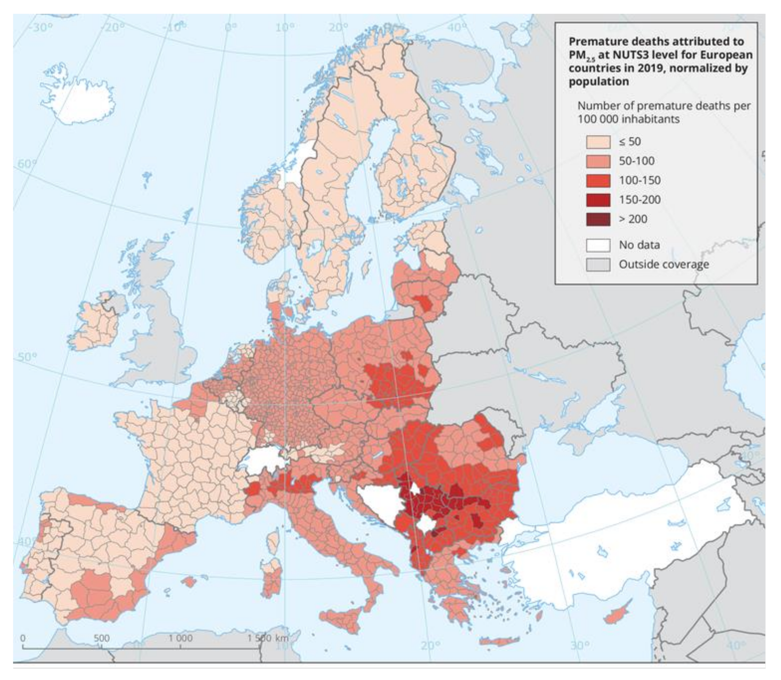
Figure 1 shows, the current state of ambient air pollution in some eastern European cities is becoming increasingly problematic where the statistics show more than 200 deaths per 100,000 inhabitants placing cities such as Sofia and Plovdiv at the highest mortality rates related to poor air quality [
2].
These highly worrying statistics call for immediate action both from a political and regulatory standpoint. However, the role of applied research solutions and comprehensive scientific analyses cannot be overlooked as they can empower decision makers and give the necessary tools to act quickly and effectively.
Both the European Union and the World Health Organization have developed air quality standards and goals. However, despite all global efforts, a survey showed that no country met the World Health Organization (WHO) air quality standards in 2021 [
3]. In order to address this highly complex problem, the European Union has created a substantial system of programs, funds and strategic plans comprising specific measures and actions in order to help countries and cities meet those standards. The implementation of those measures and actions would inevitably lead to better air quality in the long run. However, the results of these actions can take a relatively long time to take effect which leaves a gap between actions and the significant real-world mitigation of air pollution. This creates the need for the creation of tools to fill this gap and create a system for adaptation to the current levels of air pollution. An important piece of this system would be an advanced air quality forecasting tool.
To keep its inhabitants safe from harmful air, many cities have adopted air quality forecasting programs to estimate and predict the concentrations of a variety of air pollutants. Those forecasting systems give decision-makers and citizens the opportunity to take preventive measures in order to protect the most vulnerable and sensitive groups and immediately and adaptively implement measures such as temporarily stopping primary emission sources to reduce air pollution, stimulating the use of public transportation, enforcing “No-burn days”, and so on.
Accurate air quality forecasting can result in great social and economic benefits by providing the capabilities for advanced planning for citizens, families, companies and governing entities. Various analytical models are proposed for air quality prediction, which can be categorized as traditional, based on statistical models and non-traditional using Artificial Intelligence (AI) approaches. Time-series methods and regression analysis are examples of traditional techniques, while k-nearest-neighbors and artificial neural networks (ANNs) are representatives of the AI approaches. ANNs have been used in several research works for air quality forecasting [
4,
5,
6,
7,
8]. A hybrid wavelet model was developed to investigate hourly data of Taiyuan, China between 2016 and 2017 [
9]. The results show that ANNs and support vector machines (SVMs) have better forecasting accuracy on the decomposed data compared to raw data. The higher accuracy of the models on the transformed data is proved also by Cheng et al. [
10], who employed the AutoRegressive Integrated Moving Average (ARIMA), SVN and ANN methods. The requirement of less computational power, satisfactory prediction ability, relatively easy implementation and increased availability of air quality data make the regression analysis a preferable technique among the statistical methods. The time series regression is a statistical method that predicts the future based on the past, known also as autoregressive dynamics. It evaluates historical data to establish a valid forecasting model. The AARIMA method has been extensively studied and implemented in recent years, proving to be an effective approach in providing accurate results and it has been expounded in many previous publications.
In the air quality forecasting field, the time-series approach is generally used to understand the cause-and-effect relationships. The ARIMA method has been widely applied in the last few decades to analyze and predict air pollutant concentrations [
11,
12,
13,
14,
15]. One study accounted seasonal non-stationarity in time series models for short-term ozone level forecasts [
16]; and simulation of the daily average PM10 concentrations were done at Ta-Liao [
17], while another used ARIMA to forecast a full range of pollutants-ozone (O
3), nitrogen oxide (NO), nitrogen dioxide (NO
2) and carbon dioxide (CO) [
18]. Hidden periodicities of the fine particle (PM10) time series were identified and used to increase the performance of the time series models [
19]. The duration of cycle is calculated for observed PM10 levels in London as 365 days corresponding to a year, 7 days corresponding to a weak, 456 days corresponding to 15 months, and 183 days corresponding to 6 months and 25 days. In East Central Florida, nonlinear regression and ARIMA models were used for precipitation chemistry from 1978 to 1997 [
20]. The trends in PM2.5 concentrations of Fuzhou, China between August 2014 and July 2016 were studied using the ARIMA [
21]. Seasonal fluctuations of two years were identified as a result, where lower concentrations appear in warm days, while higher concentrations appear in cold days. Periodogram-based time series methodology was utilized to find the hidden periodic structure of monthly PM2.5 data, available for Paris between January 2000 and December 2019 [
22].
Different studies focus on a wide variety of applications from predicting Air Quality Index (AQI) comprising every major pollutant to individual pollutant concentrations predictions. A study in Taiwan [
23] mainly predicted multi-level AQI classifications, which helped forecast qualitative AQI at time t based on information up to t−1 when considering seasonal variables and three weather covariates: daily wind direction, daily average temperature and daily accumulated precipitation. Henry et al. [
24] located nearby sources of air pollution by nonparametric regression of atmospheric concentrations on wind direction.
Numerical air quality forecasts in Hong Kong were improved using stochastic time series approach, namely ARIMA models [
25]. The ARIMA model was used to predict fine particle (PM2.5) concentrations at the 35 air quality monitoring stations in Beijing in a span of 24 h resolving the issue of processing high-dimensional large-scale data and taking the forecasting data as one of the data sources for predicting the air quality [
26]. Acknowledging the lack of data, the study employed the sliding window mechanism to deeply mine the high-dimensional temporal features for increasing the training dimensions to millions. Another study provided an in-depth analysis of all factors of air pollutants by correlation between those factors. Using the Seasonal Autoregressive Integrated Moving Average (SARIMA) model, a prediction of future concentration of PM2.5 was made which gives the increasing value and provides the lowest and highest predictions of PM2.5 concentrations in the next year [
27].
The main goal of this study is to find trends and forecast the air pollution in Sofia City, Bulgaria thorough development of time series predictive models for different air pollutants such as CO, NO2, O3 and fine particles (PM2.5). The ARIMA method is employed for predictive analytics at five local air quality monitoring stations with the aim of improving forecast accuracy at roadside, rural and urban places.
Sofia City was chosen for the case study since it is vulnerable to air pollution due to three main factors as follows:
Geographic—The city is located in a valley surrounded by mountains, which keep the pollutants over the city for prolonged periods of time, especially during the winter, when fog and thermal inversions appear.
Urban traffic—The city has over 1 million inhabitants, and there are almost 0.8 cars per adult. The cars in Sofia are more than the average in big cities in Europe (0.5 cars per adult), and the trend for car traveling continues to grow [
28,
29].
Domestic heating—Part of the city’s population is still using solid fuel for heating, which is mostly low-quality coal producing a lot of smoke and ash [
30].
The rest of the paper is organized as follows.
Section 2 describes the methods used for data preparation and analysis.
Section 3 describes the obtained results of the air quality forecasting models.
Section 4 discusses the main findings and forecasts, while
Section 5 concludes the paper and gives directions for future work.
2. Materials and Methods
The data is collected by five air quality stations located within and near Sofia City. The air quality stations, shown in
Figure 2, are managed by the Bulgarian Executive Environmental Agency (ExEA), which is a national reference within the European Environment Agency (EEA). The data ranges from 1 January 2015 to 31 December 2019, providing values for the levels of the polluters CO, NO
2, ozone O
3, PM2.5.
Since the measurements are not available for every pollutant in all air quality stations (see
Table 1), the study is focused on the data obtained by the air quality stations at the neighborhoods of Pavlovo and Hipodruma and the region of Kopitoto, which is located close to Vitosha mountain. The measurements of PM
2.5 are available only for the neighborhood of Hipodruma.
2.1. Data Preparation
The initial raw data contains hourly measurements. Due to missing values and presence of noise in the data, both imputation and aggregation of data is performed. Granularity periods of 3 h, 6 h, 12 h and 24 h (1 day) are used.
2.1.1. Quality of Raw Data
The raw datasets are explored to check their quality. The results are summarized in
Table 2,
Table 3,
Table 4 and
Table 5. The exploratory analysis performed looks to identify the percentage of the missing and the negative values. Such missing and negative values may be due to temporary failure or bias of the sensors measuring the level of the polluter for the current time frame (1 h in the case of the current study). A threshold of 15% for missing or negative values is applied to discard the specific air quality station for the corresponding polluter. If the sum of the percentages of the missing and negative values for each line in
Table 2,
Table 3,
Table 4 and
Table 5 is equal to or above 15%, the data is considered as incomplete or of low quality and not taken for further exploratory and time series analysis.
When the threshold of 15% is applied, the data related to NO2 at “Orlov most” (85.3% of missing values) and “Mladost” (24.1% of missing values) air quality stations and the data related to CO at “Orlov most” (85.0% of missing values) and “Mladost” (18.0% of missing values) air quality stations are discarded. For the rest of the data, the negative values are fixed to 0.0, supposing that there were some bias or failure in the sensors measuring the level of the polluter in a small portion of the time frame.
2.1.2. Imputation of Missing Values
Since for the chosen method in time series analysis, applied in the current research paper, it is essential to avoid missing values, they are handled in the raw dataset after the corrections described in previous subsection. It is worth mentioning that there are methods for time series analysis that do not require imputation, if certain conditions are met [
31] and corresponding software implementations are available [
32]. However, different methods for time series imputation have been tried and some of them are included in the interpolate functionality for data frames manipulation in the programming language Python [
33] and in the more sophisticated library dedicated to missing values imputation [
34]. Besides the simpler forward and backward imputation method, linear, quadratic and spline interpolation have been applied but the results were unsatisfactory. The issue is solved by applying a method of imputation by averaging the present values by year, month, day and hour. For example, in the raw dataset for NO
2 at “Kopitoto” air quality station there are missing values for the period from 4 p.m. 20 August 2015 until 6 p.m. 14 September 2015. Thus, all the values from the same time frame for the years 2016, 2017, 2018 and 2019 are taken to substitute the missing values. Since the data for these years in this time frame may again have missing values, only the present ones are used, and the missing values are filled by averaging of the values for the corresponding slot in the selected time frames.
2.1.3. Data Granularity
For the purpose of the study, data is aggregated using granularity of 3 h, 6 h, 12 h, 24 h (1 day). The time stamp for each aggregated value is taken from the end of the granularity period. For every present polluter and air quality station the data is aggregated, and separate forecasting time series models are created for each combination of polluter, district and granularity of data.
2.2. Analytical Methods
ARIMA (p, d, q) (P, D, Q) model is applied to perform data analysis, where p, d, q and P, D, Q represent continuity and seasonal auto-regression differences, respectively. It consists of three components Autoregressive (AR) model, Integrated (I) and Moving Average (MA) model. AR and MA are combined on data differenced for stationarity. Autocorrelation function (ACF) and Partial Autocorrelation (PACF) are used to select the best values for the models’ parameters.
2.2.1. Autocorrelation and Partial Autocorrelation
In order to identify how the observations are correlated in the time series, the autocorrelation is used. The correlation coefficient is plotted by the ACF against the lag measured in terms of periods. The lag is related to a certain observation in time after which the first value is observed in the time series. Thus, ACF is calculated by the autocovariance of
and
as follows [
35]:
where
is a covariance of variables
and
, and
is a variance of the variable
. The covariance measures the relationship between two random variables, while the variance measures the variability The correlation coefficient ranges from −1 (negative relationship) to 1 (positive relationship). If there is no relationship between the variables, the correlation coefficient is 0.
Partial autocorrelation summarizes the relationship between an observation and observations at prior time period without taking into account the correlations between the intervening observations. The PAC is a simple correlation of
and
, which can be calculated as follows [
36]:
where
is the expected value of
. The optimal solution model for the time series is obtained according to the results from ACF and PACF.
2.2.2. Stationarity
The stationarity of a time series is an important condition that is required by the majority of time series forecasting algorithms. The stationarity means that the statistical characteristics of the time series such as mean, variance, autocorrelation, etc. do not change over time. In case of missing stationarity, the time series need to be stabilized before further analysis. A Stable History Period (SHP), namely a time period when the time series remain stable, can be used to resolve such issue [
31]. The stability of the time series in this study is determined by ACF and PACF. Time series is stable, if ACF fluctuates around a fixed horizontal line with a gradual decay trend.
A differential transformation can be applied to the time series
to produce stationary time series
[
26] as follows:
An alternative approach is to calculate the percent of change, as follows:
For example, the time series of CO can be non-stationary, and a differential transformation can be applied to achieve stationarity. The first-order differencing determines the difference in observations between two subsequent periods. If stationarity is not achieved, a second-order differencing is applied on the first-order differencing. The process can be repeated until the time series become stationary.
2.2.3. ARIMA Method
The ARIMA employs an AR model in combination with a MA model to perform time series forecasting. The main parameters considered are as follows:
Number of previous observations (p);
Degree of differencing (d);
Size of the moving average (q).
The AR model shows the dependence of one observation on an earlier time period. The AR model obtains
p previous observations as follows [
36]:
where
is predictand for time t from a normal distribution and
defines p previous observations of the same time series.
denotes the regression coefficients,
is a constant and
is the random error term. The order
p for the AR(
p) model is selected based on the significant spikes of PACF. An additional indicator is the slow decay of ACF.
The MA performs forecasting relying on moving averages of the past random error terms as follows:
where
represents the regression coefficients,
q is the order of moving average, and
is a constant. The order
q for the MA(
q) model is obtained from the ACF, if it has a sharp cut-off after lag
q. The PACF decays slowly in this case.
The ARIMA model can be defined as follows:
where
B is a backshift operator,
p is the order of autoregression,
d is the order of differencing and
q is the order of moving average.
2.2.4. Evaluation Metrics
The best combination of
p and
q can be found using an objective function, which can measure the performance of the model on a validation set. Akaike Information Criteria (AIC) and Bayesian Information Criteria (BIC) are mathematical methods for scoring statistical models and selection of one that best one in a candidate model space. AIC evaluates the model’s goodness-of-fit to the data, as follows [
37]:
where
l is a log-likelihood, and
k is a number of parameters in the candidate model. Additional indicator
n is added to the BIC, which defines the number of samples used for fitting as follows [
27]:
The BIC is derived under Bayesian network, while the AIC is elaborated by adjusting biased empirical information. It tends to select a less complex model in comparison to AIC. The coefficient of determination, called R-squared, measures the proportion of the variance of the dependent variable, predictable form the dependent variables in the model. It can also be used for evaluation of the model’s goodness-of-fit to the data. R-squared varied between 0% and 100%, where 0% means that the model does not explain the variability of the response data around its mean and 100% means that the model explains all the variability.
2.2.5. Software Libraries
The air quality models are implemented using the Python programming language and libraries matplotlib and seaborn for data visualization and pandas, numpy and statsmodel for the data analysis.
3. Experimental Results
The results from the exploratory analysis of the data are shown in
Figure 3 and
Figure 4.
3.1. Analytical Methods
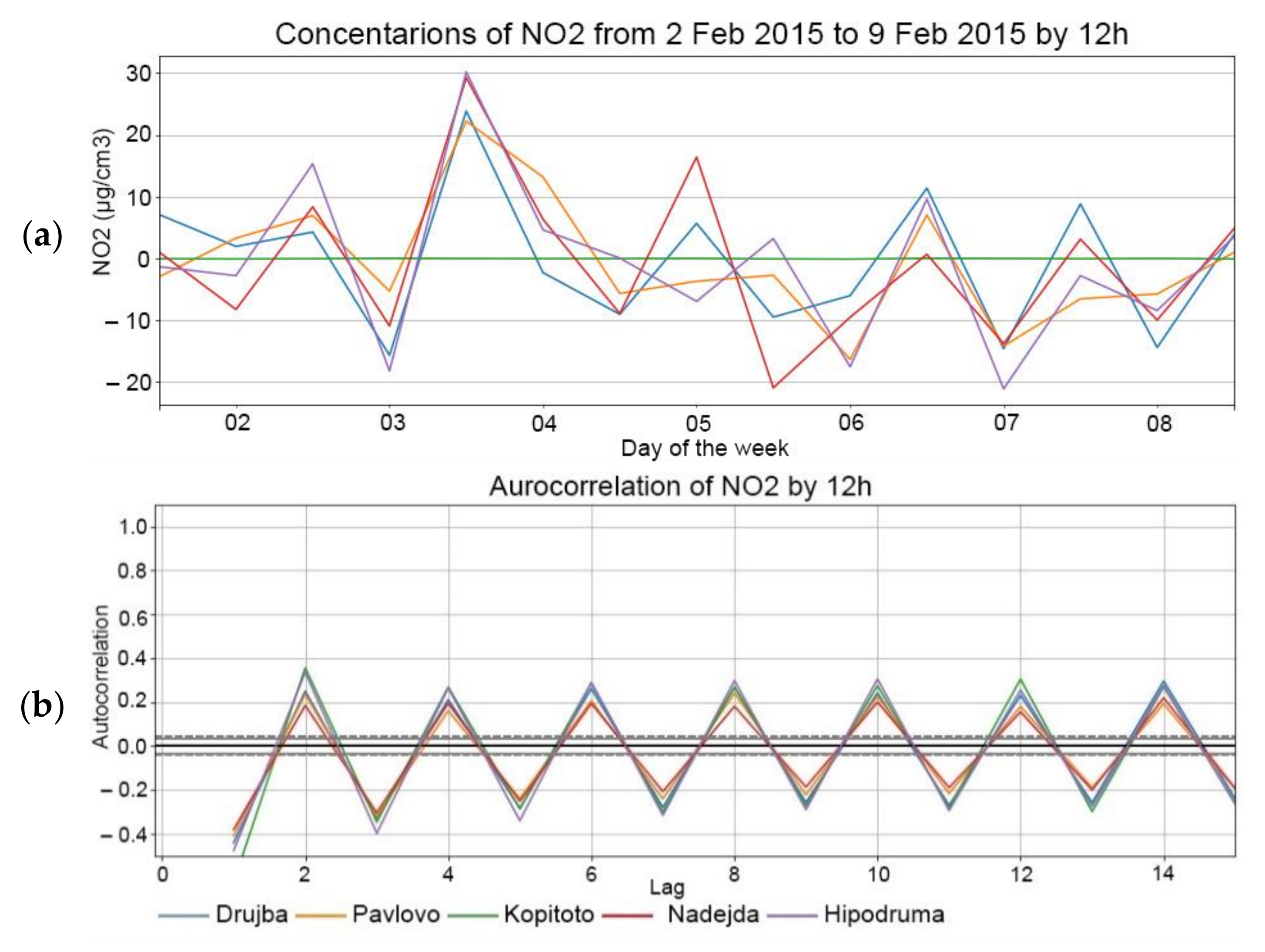
Figure 5,
Figure 6 and
Figure 7 show that there are some seasonalities for the NO
2 data aggregated by 1 h, 3 h and 12 h. The plot of
Figure 5 shows a seasonality with lag 24, corresponding to the pick in the autocorrelation lower part, and that is expected because of the repeated daily activity by hour within the city. The second significant pick is observed 24 h after the first one, and namely, near the 48th tick. A similar trend is observed in
Figure 6 and
Figure 7 and the most significant picks in the autocorrelation part of the plots are at 24/3 = 8 and 24/12 = 2, respectively. As expected, the second significant picks shown in for
Figure 6 and
Figure 7 are observed at the 16th and 4th ticks, which corresponds to the 2-day lags after the first tick.
For the sake of brevity, plots for NO2 are shown only but one observes similar behavior for the rest of the pollutants.
Partial autocorrelation, as described in
Section 2.2.2, was also applied to check what is the direct relation of lagged members to the first member of the series (without taking into account the ones in between).
Figure 8 presents an example for NO
2 measurements in Drujba air quality station. It can be seen that for one 1 h aggregated data there is a direct relationship of the members of the series at and immediately before the 24th tick, which is expected since the granularity of the data by hour and the daily activities withing the city. Similar behavior can be observed in the plots corresponding to the 3 h and 12 h granularity of the data. There are direct relationships of the first lag and the lags on and immediately before the 24/3 = 8th lag for 3 h granularity and the first lag and the lags on and immediately before the 24/12 = 2nd lag for the 12 h granularity. Similarly, as in the autocorrelation part, further picks are observed in the partial autocorrelation plots, which are located immediately before the 48th, 6th and 4th lags.
As described in
Section 2.2.2, two statistical tests are used to check for (non) stationarity of the signals, namely the augmented Dickey–Fuller (ADF) and the Kwiatkowski–Philips–Schmidt–Shin (KPSS) tests. A common misconception is that both tests can be used interchangeably, which can lead to contradictory conclusions about the stationarity of the tested signal. A key difference between ADF and KPSS is how one states the null hypothesis and consequently the interpretation of the
p-value, which is the opposite in each other.
The ADF test should be interpreted as follows:
If p-value > 0.05 (test value > 5% test critical value), one fails to reject the null hypothesis (H0) and the data is considered as non-stationary;
If p-value ≤ 0.05 (test value ≤ 5% test critical value), one rejects the null hypothesis (H0) and the data is considered as stationary.
On the other hand, the p-value of the KPSS test is interpreted in the opposite side.
The critical values for ADF test are 1% (−3.430), 5% (−2.862), 10% (−2.567) and for the KPSS test: 1% (0.739), 5% (0.463), 10% (0.347).
The results of applying both tests on the data into consideration are stated in
Table 6,
Table 7 and
Table 8.
The Python’s library statsmodels is used, where the output for ADF and KPSS tests is:
Value of the test statistic
The p-value
Number of lags considered for the test
The critical value cut-offs
For the purpose of the current paper, we consider the typical critical test value 5%, that is, p-value of 0.05. Based on the assumptions made for the ADF and KPSS tests, the main observation is that even without significant analytical transformation on the signal for NO2, for all levels of granularity except Kopitoto for KPSS, all other air quality stations show significant level of signal stationarity. Additionally, that significant stationarity is confirmed by both tests. That is, for all considered air quality stations, the ADF p-value < 0.05, and again for all air quality stations except Kopitoto, the KPSS p-value > 0.05. Furthermore, the last consideration is valid not only for the 5% critical values of the corresponding tests, but also for the further 10% critical values. However, for the station obtained from Kopitoto and the KPSS test, we observe that for all levels of granularity, the test statistic > critical% value and p-value < 0.05, which rejects the null hypothesis, and we conclude that the signal is rather non-stationary.
As a conclusion, both tests show significant levels of stationarity for all air quality stations except Kopitoto. For Kopitoto, ADF shows stationarity and KPSS shows non-stationarity. Therefore, the series for Kopitoto are non-stationarity to some extent and lag difference is to be used to make the series more stationary.
Lag difference for the 1 h, 3 h and 12 h granularity of the initially preprocessed data is applied. The number of lag differences for the corresponding granularity levels are based on the observations regarding the autocorrelation and partial autocorrelation plots. The results after applying the lag difference procedure on the corresponding signals and their autocorrelation plots are shown in
Figure 9,
Figure 10 and
Figure 11. The plots clearly show the improvement of stationarity compared to the plots in
Figure 5,
Figure 6 and
Figure 7.
Figure 12 shows the partial autocorrelation of NO2 in “Drujba” air quality station measured at 1 h, 3 h and 12 h granularity with lag difference 1. Numerically, the improvement of stationarity levels after applying the lag differences are shown in
Table 9, where one can check the ADF and KPSS tests applied on the NO
2 dataset for granularities: 1 h with lag difference 24, 3 h with lag difference 8 and 12 h with lag difference 2. In
Table 6, only the corresponding test values are shown, where the improvement consists of the reduction of the values of ADF and KPSS tests for the corresponding data granularities and lag differences. For Kopitoto air quality station, the KPSS test, having shown non-stationarity with critical
p-value 0.05 before, after the lag difference, has a test value significantly lower than the critical test value. Therefore, the lag difference turned the signals corresponding to Kopitoto from non-stationary to stationary for all granularity levels.
3.2. ARIMA Models
There is a rule of the thumb on how to choose the parameters for AR (
p), lag difference (
d) and MA (
q). From the autocorrelation graphs one may conclude that there is a significant number of consequent positive lags; therefore, one needs to apply more differencing and, on the other hand, if more lags are negative, the series may be over-differenced already. Higher degree lag differences have been tested but they produced too many negative autocorrelation lags. Therefore, for that data more than 1 degree lag difference may not be needed. The parameter p can be chosen to correspond to the most significant lag in the partial autocorrelation plot. From
Figure 11, one concludes that
p = 7 may be a good choice for 1 h granularity, and 2 and 1 for 3 h and 12 h granularity, respectively. The parameter q, corresponding to the MA degree can be chosen roughly by counting the number of lags crossing the threshold of −0.2/+0.2 threshold in the autocorrelation plots. Therefore, for 12 h and 3 h granularity q can be chosen larger compared to 1 h granularity.
Because the above rule is not mathematically grounded, a grid search is applied based on the Python’s library pmdarima. For the grid search of the parameters the AIC and BIC metrics were used in combination with the ADF test. As a final evaluation metric mean absolute error (MAE) is applied.
Figure 13 and
Figure 14 present plots with predictions from ARIMA models of NO
2 for optimally chosen parameters p, d and q for granularity 1 h and 3 h, respectively.
Table 10 shows the corresponding numerical values.
The results for CO in the stations located in the neighborhoods Hipodruma, Pavlovo and Kopitoto passed through the same grid search and ARIMA based time series analysis pipeline are presented in
Table 11.
4. Discussion
The ARIMA method is one of the most commonly used ones to forecast the future values of time series. The predictions obtained from the application of this method would converge the mean of the time series for a further period if a stationarity is ensured [
17]. The ARIMA method gives consistent results for short-term predictions. It is not preferable for long-term predictions, especially in the case of periodicity in time series. Long-term predictions, e.g., annual, might be more useful for city authorities to define long-term policies and measures. Thus, the periodicity of the time series has to be considered in order to provide reasoning based on the hidden data cycles. The knowledge about the underlying structure can be used as the measurement of effectiveness of the measures taken by policy makers [
21].
ADF and KPSS statistical tests are used to check stationarity of the data for granularities of 1 h with lag difference from 1 until 24, 3 h with lag difference from 1 until 8 and 12 h with lag difference 1 and 2. Both tests show significant level of stationarity in NO
2 measurements for all air quality stations except “Kopitoto”, where ADF shows stationarity and KPSS shows non-stationarity. The stationarity levels are improved after applying the corresponding optimal lag differences for all granularity levels, obtained from the Python’s library pmdarima and optimizing the ADF statistics. The inter- and intra-annual fluctuations in data could be further explored by the least-squares wavelet analysis (LSWA), which avoids interpolation and/or gap filling and decomposes the time series into the time-frequency domain [
32]. The SHP representing both inter- and intra-annual fluctuations can be successfully determined in the time series [
31]
The ARIMA method is successfully applied to perform forecasting of the air pollutants considering different granularities. The developed ARIMA models show the powerfulness of the time series to predict pollutant concentrations. They work quite well, as it can be seen in
Figure 13 and
Figure 14, especially for 1 h granularity. The verification of the results show that the predicted values are close to the actual ones. The mean absolute error varies between 1.52 and 5.12 for 1 h granularity and 2.53 and 14.12 for 3 h granularity. The ARIMA method often outperforms sophisticated structural methods with short-term predictions for one-step forecasting on univariate datasets. Therefore, the developed ARIMA models within this study can be used as a benchmark for evaluation of different forecasting methods. They also can be combined with other techniques fully mine time series characteristics [
38].
The ARIMA method requires data on time series in question only. This is an advantage, especially in case of large volume of time series as it is in the current case. Thus, it is simple and efficient. Furthermore, additional predictive methods will be explored, such as Long Short-Term Memory [LSTM], which are proven to provide predictions closer to ARIMA [
4].


