The Role of Emission Sources and Atmospheric Sink in the Seasonal Cycle of CH₄ and δ¹³-CH₄: Analysis Based on the Atmospheric Chemistry Transport Model TM5

Abstract

This study investigates the contribution of different CH₄ sources to the seasonal cycle of ${\delta }^{13}$C during 2000–2012 by using the TM5 atmospheric transport model, including spatially varying information on isotopic signatures. The TM5 model is able to produce the background seasonality of ${\delta }^{13}$C, but the discrepancies compared to the observations arise from incomplete representation of the emissions and their source-specific signatures. Seasonal cycles of ${\delta }^{13}$C are found to be an inverse of CH₄ cycles in general, but the anti-correlations between CH₄ and ${\delta }^{13}$C are imperfect and experience a large variation ($p=$−0.35 to −0.91) north of 30° S. We found that wetland emissions are an important driver in the ${\delta }^{13}$C seasonal cycle in the Northern Hemisphere and Tropics, and in the Southern Hemisphere Tropics, emissions from fires contribute to the enrichment of ${\delta }^{13}$C in July–October. The comparisons to the observations from 18 stations globally showed that the seasonal cycle of EFMM emissions in the EDGAR v5.0 inventory is more realistic than in v4.3.2. At northern stations (north of 55° N), modeled ${\delta }^{13}$C amplitudes are generally smaller by 12–68%, mainly because the model could not reproduce the strong depletion in autumn. This indicates that the CH₄ emission magnitude and seasonal cycle of wetlands may need to be revised. In addition, results from stations in northern latitudes (19–40° N) indicate that the proportion of biogenic to fossil-based emissions may need to be revised, such that a larger portion of fossil-based emissions is needed during summer.

1. Introduction

Methane (CH₄) is a greenhouse gas of which the abundance is influenced by anthropogenic activities. It causes 28 times more radiative forcing (global warming potential) than equal mass emissions of CO₂ when integrated over 100 years [1]. The abundance of CH₄ in the atmosphere has more than doubled since pre-industrial times [2]. CH₄ is emitted to the atmosphere from thermogenic, pyrogenic, and biogenic sources, which can be natural or anthropogenic in origin [3]. Most of the seasonal cycle of CH₄ emissions are driven by the pyrogenic and biogenic sources, such as biomass burning, wetlands, and rice cultivation [4,5,6,7,8]. The processes are highly dependent on climatological and meteorological conditions, such as temperature and precipitation, and cultivation cycles. In contrast, thermogenic sources, such as fossil fuel extraction and distribution, have little month-to-month variation, although winter emissions may be greater in some regions due to the consumption of natural gas for heating [4]. Likewise, instantaneous perturbations in emissions may occur due to blowout events from natural gas wells [9,10].

Seasonal variations in wetland CH₄ emissions have been studied intensively by site-level measurements, e.g., [11,12], process-based land surface ecosystem models, e.g., [13], and atmospheric inversions, e.g., [14,15], but there are still high uncertainties in the magnitude and timing of maximum emissions on continental to regional scales [5,16,17]. Anthropogenic CH₄-emission seasonal cycles also have uncertainties. Although some countries report emission magnitudes to, e.g., the UNFCCC, often only annual values are reported. However, emissions from rice paddies, for example, may not properly consider temperature dependencies and soil properties [18]. In addition, emissions from livestock (e.g., enteric fermentation and manure management) may have seasonal cycles depending on temperature [19]. However, again, such information is often not included in the reported emissions, and only few global inventories take the seasonal changes from this sector into account ([4] and references therein).

CH₄ has two stable carbon isotopes, ¹²C and ¹³C, and hydrogen isotopes, ¹H and ²H. For the carbon isotopes, their process-specific isotopic signatures (¹³C/¹²C ratio compared to a reference, denoted as ${\delta }^{13}$C) depend on processes that produce CH₄ [20]. Generally, emissions with pyrogenic origin are most enriched in ¹³C, followed by thermogenic sources. Sources from biogenic origin are most depleted in ¹³C, e.g., [20,21]. Such information has been shown to be useful in quantifying CH₄ source distributions [22,23,24,25], in addition to CH₄-only atmospheric inversions, which estimates total CH₄ budgets, e.g., [3,26]. However, the CH₄ flux information derived using the information from isotopic measurements still suffers from high uncertainty, as the isotopic measurements are still limited in both spatial and temporal coverage, and partly overlapping signatures make source divisions uncertain [22]. On top of that, the isotopic signature of emissions can vary significantly by location due to differences in production processes, types of origin, or methanogenesis [27,28,29,30]. In Ganesan et al. [27], the authors cautioned that emission quantification, including its seasonality, without fully incorporating detailed spatial information of the isotopic signatures may lead to erroneous results.

The seasonal cycle of ${\delta }^{13}$C is determined by atmospheric sinks and emissions. Sinks enrich the atmosphere in the ¹³CH₄ due to their kinetic isotopic effect (KIE), and they have a strong seasonality, mainly due to the seasonality of OH radicals in the troposphere and of Cl and O(¹D) in the stratosphere. The KIE is the difference in the reaction rate between the isotopes. In addition, the fractionation factor by OH differs between studies [31,32]. The fractionating factor describes the relative partitioning of the heavier (carbon-13) and lighter (carbon-12) isotopes.

In general, the ${\delta }^{13}$C cycle is mirroring, i.e., in an opposite phase of, the CH₄ cycle in high southern latitudes, where the effect of emissions is small [31,33]. However, the ${\delta }^{13}$C cycle is known to be affected by the seasonal variations in emissions, where most of the emissions are depleted in ¹³CH₄. Therefore, the ${\delta }^{13}$C cycles do not correlate well with the atmospheric CH₄ cycles, especially in the Northern Hemisphere (NH) [34,35,36]. Studies found that the ${\delta }^{13}$C seasonal cycle reaches its maximum approximately two months earlier than CH₄ reaches its minimum in the NH. Studies using inverse transport modeling indicate that the weak negative correlations and phase shifts are strongly influenced by wetlands in the northern high latitudes and biomass burning in the tropics [16,34,35,37]. The role and magnitude of the tropospheric Cl sink is also uncertain, ranging from 13–37 [38] to 12–13 Tg CH₄ yr ${}^{-1}$ [39] to even smaller estimates [40]. The estimated magnitude of the soil sink also varies; from bottom-up estimates, it is 11–49 Tg CH₄ yr ${}^{-1}$, and it is 27–45 Tg CH₄ yr ${}^{-1}$ from top-down estimates ([3] and references therein).

In this study, we revisit the topic of the seasonal cycle of the ${\delta }^{13}$C and CH₄ source and sink contributions, earlier discussed in, e.g., Allan et al. [34] and Bergamaschi et al. [35]. Since previous studies, there have been updates on source-specific isotopic signatures, including spatial variations, e.g., [21,22,27,28,29], and new ${\delta }^{13}$C observations are available. Additionally, the atmospheric transport model has improved significantly compared to earlier versions used by Allan et al. [34] and Heimann [41], e.g., with finer resolutions and improved chemistry schemes [42,43]. The previous studies of the seasonal cycle of ${\delta }^{13}$C [16,34,35] have mainly covered natural emissions, but the latest information on the seasonal cycle of anthropogenic emissions is now available [4,44].

We examined the average ${\delta }^{13}$C seasonal cycle for 2000–2012 as well as the CH₄ source and sink contributions at 30° latitudinal bands based on the TM5 global atmospheric transport model. We estimated atmospheric CH₄ and ${\delta }^{13}$C cycles using the most recent isotopic signatures published, including spatial variations. We also used emission fields with different seasonality, including those from anthropogenic sources, and examined the differences in the combined CH₄ and ${\delta }^{13}$C cycles. The examination of the seasonal cycle of ${\delta }^{13}$C provided information on the seasonality of different emission categories. In addition, we evaluated the seasonal cycle of anthropogenic emissions and the possible problems presented by the two recent versions of the EDGAR inventories, v4.3.2 and v5.0, by comparing them with observations from the National Oceanic and Atmospheric Administration Global Monitoring Laboratory (NOAA/GML) and the Institute of Arctic and Alpine Research (INSTAAR). Comparison with the observations helped to identify which EDGAR version is more realistic. The EDGAR v4.3.2 data availability is limited to 2012, so our study period was chosen to be 2000–2012. The purpose of this study was to attain a better understanding of ${\delta }^{13}$C distributions and how different CH₄ sources contribute to the seasonal cycle of ${\delta }^{13}$C. This also raises the need for future studies to be conducted by inverse modeling.

2. Materials and Methods

2.1. The TM5 Atmospheric Chemistry Transport Model

TM5 [42] is a global Eulerian atmospheric chemistry transport model. It is driven by ECMWF ERA-Interim meteorological fields, which for this study is run on a 1° × 1° (latitude × longitude) zoom grid over Europe (up to 74° N, Figure S1) embedded in a 4° × 6° global grid with an intermediate 2° × 3° zoom region, e.g., [45]. Vertically, 25 layers are used, corresponding to a subset of the original 60 ERA-Interim layers. Convective vertical mixing was calculated based on the Gregory et al. [46] convection scheme archived in the ERA-Interim meteorological fields.

In this study, CH₄ (including ¹²CH₄ and ¹³CH₄) and ¹³CH₄ are transported as two separate tracers, and ¹³C-CH₄ (${\delta }^{13}$C) is calculated as follows:

$$\delta {}^{13}\mathrm{C}\text{-}\mathrm{C}{H}_4=\left(\frac{{({}^{13}\mathrm{C}/{}^{12}\mathrm{C})}_{\mathrm{sample}}}{R_{\mathrm{std}}}-1\right)\times 1000,$$

(1)

where $R_{\mathrm{std}}=0.0112372$ is the isotopic (¹³C and ¹²C) ratio of the Vienna Pee-Dee Belemnite (VPDB; [47]) standard.

The atmospheric sink in TM5 includes off-line chemistry; chemical reactions with OH, Cl, and O(¹D) are prescribed, but the model does not have full chemistry. The reaction with OH, the largest sink of atmospheric CH₄, is calculated based on the procedure presented by Houweling et al. [26]. The monthly variations in OH concentrations are based on Spivakovsky et al. [48], and the total OH concentration scaled by 0.92 based on an evaluation using methyl chloroform [43]. The first-order loss rates for the reactions with Cl and O(¹D) are considered only in the stratosphere, where the reaction rates are prescribed based on the atmospheric chemistry general circulation model ECHAM5/MESSy1 [49]. No interannual variation of the photochemical sink processes is included in this study, because we assumed that the OH is well-buffered and thus unchanging [20,22,50,51,52]. Note also that the study aims to analyze the seasonal cycle but not trends and interannual variations in the CH₄ and ${\delta }^{13}$C.

Kinetic isotopic effects (KIEs) k(¹²CH₄)/k(¹³CH₄) of 1.004 and 1.013 are used for ¹³CH₄ OH and O(¹D), respectively [31], and 1.066 [53] is used for Cl. In this study, the KIE of total CH₄ was assumed to be the same as for ¹²CH₄, i.e., k(¹²CH₄)/k(¹³CH₄) ≈ k(CH₄)/k(¹³CH₄).

In addition to the photochemical sinks, we included the sink to dry soils (i.e., a negative flux from atmosphere to soil) in the lowermost layer of TM5. CH₄ is oxidized by bacteria in aerobic mineral soils, so the sink depends on soil moisture, temperature, and soil texture [54]. These dependencies lead to the smallest sink in winter and the largest sink in the summer (Figure 1). The soil sink can be treated as a pseudo first-order reaction $L=k^{\prime }·\left[\begin{array}{c}\hfill \mathrm{C}{\mathrm{H}}_4\end{array}\right]$, where $k^{\prime }=k/h$, and h is the thickness of the lowermost layer. The flux F at the soil surface is $F=k·\left[\begin{array}{c}\hfill \mathrm{C}\mathrm{H}4\end{array}\right]$. The ¹²CH₄ soil sink $F_{\mathrm{soil},12}$ is taken from the LPX-Bern v1.4 land ecosystem process model [55] and varies interannually (32.7–33.8 Tg CH₄ yr${}^{-1}$) and monthly. The removal rate of ¹²CH₄ is then $L_{\mathrm{soil},12}=1/h·F_{\mathrm{soil},12}$. The removal rate for ¹³CH₄ due to the soil sink, $L_{\mathrm{soil},13}$, is therefore calculated as

$$L_{\mathrm{soil},13}=\frac{F_{\mathrm{soil},12}}{h·{\mathrm{KIE}}_{\mathrm{soil}}}\times \frac{\left[{}^{13}\mathrm{C}{\mathrm{H}}_4\right]}{\left[{}^{12}\mathrm{C}{\mathrm{H}}_4\right]}$$

(2)

where $F_{\mathrm{soil},12}$ is the negative flux of ¹²CH₄ at the surface, h is the thickness of the lowermost layer, [¹²CH₄] and [¹³CH₄] are the atmospheric concentrations of ¹²CH₄ and ¹³CH₄, and KIE ${}_{\mathrm{soil}}$ is assumed to be 1.0177 [56].

TM5 has been applied to various CH₄ studies, and initial three-dimensional (3D) CH₄ fields were readily available from, e.g., our previous study by Tsuruta et al. [45]. For ¹³CH₄, spin-up was needed to create 3D mixing ratio fields that are in an approximate steady state. We ran 40 years of spin-up (running TM5 using emissions and meteorological fields of year 2000 for 40 times) starting from the converted fields and based on the emissions and isotopic signatures described in Section 2.2 and Section 2.3. During the spin-up, the stratospheric ${\delta }^{13}$C increased by ∼20‰, reaching approximately −10‰ at the end of the spin-up, which is close to that of previous studies [31,57]. In this study, the focus is on the troposphere. However, we acknowledge that the troposphere and the stratosphere are linked through stratosphere–troposphere exchange [58], and we briefly return to the simulated stratospheric concentrations and effects of the exchange in the discussion.

2.2. CH₄ and ¹³CH₄ Flux Fields

The global CH₄ flux fields from anthropogenic and natural sources were taken from inventory and process-based model data (Section 2.2.1 and Section 2.2.2). All fields were pre-processed to a global 1° × 1° grid to match the TM5 model resolution. ¹³CH₄ fluxes were calculated by converting CH₄ flux fields using the isotopic signature (

Table 1. Isotopic signatures used to convert CH₄ flux fields to ¹³CH₄ fields. For values spatially varying globally, ranges of values are shown. Please see Supplementary Figure S3 for spatial distributions. Isotopic signatures from Monteil et al. [24] are also presented for comparison.

Emission Source	Signature Value (‰)	Signature Value (‰)
	(Used in This Study)	[24]
Enteric Fermentation and Manure Management (EFMM)	[−67.9, −54.5] 1, −66.8 2	−62
Landfills and Wastewater Treatment (LWW)	−55.6 2	−55
Rice (RICE)	−62.1 2	−63
Coal	[−64.1, −36.1] 1, −40 2	−35
Oil and Gas	[−56.6, −29.1] 1, −40 2	−40
Residential	−40 2	−38
Wetlands	[−74.9, −50] 3, −61.3 2	−59
Fires	[−25, −12] 1, −22.2 2	−21.8
Ocean	−47 2	−59
Termites	−65.2 2	−57
Geological	[−68, −24.3] 4, −40 2	−40

¹ Feinberg et al. [28], ² Thompson et al. [23], ³ Ganesan et al. [27], ⁴ Etiope et al. [29].

) and Equation (1), such that ¹³CH₄ is solved from Equation (1), and the isotopic signature (${\delta }^{13}$C) was taken from Table 1.

2.2.1. Anthropogenic CH₄ Flux Data

Monthly global anthropogenic emissions were taken from EDGAR inventories, accessed date 23 May 2022 (https://edgar.jrc.ec.europa.eu) v4.3.2 [44] and v5.0 [4]). The original resolution is 0.1° × 0.1° (latitude × longitude), and the inventories are based on the geographical distribution of different activities, e.g., energy, agricultural land use, and traffic, utilizing GIS techniques.

The EDGAR database includes emissions from the Intergovernmental Panel on Climate Change (IPCC) 1996 [59], Classes 1, 2, 4, 6, and 7, listed in Table S1. We categorized these classes into six components: enteric fermentation and manure management (EFMM), landfills and wastewater treatment (LWW), rice cultivation (RICE), coal, oil and gas, and residential (Table S2). Among these, EFMM, LWW, and RICE are anthropogenic biogenic sources, with depleted ${\delta }^{13}$C isotopic signatures, while the others are fossil-based sources that are enriched in ¹³CH₄ [60]. The seasonal cycle of anthropogenic sources is dominated by biogenic sources. No significant seasonality is present in the fossil-based sources (Figure 1).

V4.3.2 is the first EDGAR inventory to include seasonality. It provides monthly values for 2010. We calculated the seasonal cycle for each 1° × 1° grid by applying the 2010 seasonality to other years, keeping the annual totals as the original for each year. For v5.0, monthly values for the year 2015 are available, and we applied its seasonality for each grid similarly to the procedure for v4.3.2.

The two EDGAR versions differ significantly in their seasonal cycles of EFMM and RICE (Figure 1). The EFMM emissions have a seasonal cycle in EDGAR v4.3.2, which is not included in v5.0 (Figure 1,

Table 2. Average global emission (Tg CH${}_4$ year ${}^{-1}$) and emission amplitude (Tg CH${}_4$ month ${}^{-1}$) over years 2000–2012 with range, and the months when seasonal minimum and maximum occurs. For EDGAR components, those for 2010 and 2015 for v4.3.2 and v5.0 are shown, respectively. For natural sources, the variation shows those between different years. Those marked with “*” do not have monthly variations. Note that geological emissions are kept constant during the simulations.

Data Source	Component	Emission	Amplitude	MIN	MAX
EDGAR v4.3.2	Enteric Fermentation and Manure Management (EFMM)	109.5 [102.1, 115.8]	7.50 [7.19, 7.75]	Nov	Mar
	Landfills and Wastewater Treatment (LWW)	63.8 [59.3, 68.5]	*	*	*
	Rice (RICE)	35.0 [32.4, 37.6]	2.61 [2.39, 2.74]	Jan, Dec	Mar.
	Coal	29.8 [21.9, 38.2]	0.03 [0.001, 0.11]	Jul	Jan
	Oil and Gas	68.2 [61.3, 77.1]	0.07 [0.01, 0.23]	Jul	Nov
	Residential	12.9 [12.1, 13.5]	0.78 [0.75, 0.81]	Jul	Jan
	Total	319.0 [291.3, 350.8]	10.05 [9.55, 10.41]	Nov	Mar
EDGAR v5.0	Enteric Fermentation and Manure Management (EFMM)	108.5 [102.0, 114.8]	*	*	*
	Landfills and Wastewater Treatment (LWW)	71.4 [66.6, 76.5]	*	*	*
	Rice	35.1 [32.6, 37.3]	5.51 [5.1, 5.83]	Mar	Aug
	Coal	29.5 [21.4, 38.2]	*	*	*
	Oil and Gas	67.5 [61.1, 77.4]	0.10 [0.04, 0.25]	Sept	Jan
	Residential	12.5 [12.1, 12.8]	1.65 [1.58, 1.72]	Sept	Jan
	Total	324.5 [297.7, 356.8]	5.13 [4.72, 5.47]	Mar	Aug
LPX-Bern v1.4	Wetland	157.3 [150.6, 165.7]	8.1 [6.12, 10.0]	Nov, Dec	Jul, Aug
LPX-Bern v1.4	Soil sink	33.0 [32.6, 33.7]	0.98 [0.89, 1.03]	Jul	Jan, Feb
GFED v4.2	Fires	14.4 [11.3, 19.7]	2.49 [1.07, 3.95]	Feb–Apr, Nov	Jun–Aug
Tsuruta et al. (2017)	Ocean	7.72 [7.52, 8.1]	0.08 [0.06, 0.1]	Feb, Apr–Jun, Nov	Jan, Mar, Jul, Aug, Oct, Nov
Etiope et al. (2019)	Geological	5.0	*	*	*
Ito and Inatomi (2012)	Termites	20.8 [20.8, 20.9]	*	*	*

). Both versions have seasonality in RICE emissions, but they differ significantly in the peak-to-peak amplitude and in the timing of the seasonal minimum and maximum (Figure 1, Table 2). The average amplitude of v5.0 is more than double that in v4.3.2 (Table 2). The differences in seasonality are mostly due to the following: In v4.3.2, the seasonality varies over latitude bands; in v5.0, it varies by the country for which information is available [4]. In addition, in v4.3.2, the same temporal profiles are used for all agricultural sectors, which is revised in v5.0 to better correspond to each sector separately [4,44].

Annual totals of the two versions also differ slightly. The largest difference is in the LWW (Table 2). The global total average EFMM emissions are 1 Tg CH₄ year ${}^{-1}$ larger in EDGAR v4.3.2 compared to v5.0. Both EDGAR versions have similar trends dominated by increasing emissions in EFMM, LWW, coal, and oil and gas (Figure S2). Note, however, that this study focuses on the seasonal cycle and that the analysis of trends will be presented in follow-up studies. The 2000–2012 average annual total non-biogenic (coal, oil and gas, and residential) emissions are similar in both versions, but the biogenic (EFMM, LWW, and RICE) emissions are higher in v5.0 (Table 2). This results in mean biogenic-to-non-biogenic ratios of 1.89 and 1.97 in v4.3.2 and v5.0, respectively.

In addition to the two versions of the EDGAR emissions, we created emission fields based on v4.3.2 but removed the seasonal cycle of EFMM by taking annual means. This was used to test the effect of seasonally varying EFMM emissions, which was largest in v4.3.2, but absent in v5.0.

2.2.2. Natural CH₄ Flux Data

Natural sources include those from wetlands, biomass burning, open ocean, termites, and geological sources. Among these sectors, emissions from wetlands and termites are biogenic sources with depleted ${\delta }^{13}$C values, while others are considered non-biogenic with more enriched ${\delta }^{13}$C values (Table 1). Monthly wetland emissions are taken from the process-based land ecosystem model LPX-Bern v1.4 [55], which is a dynamic vegetation model that estimates fluxes for wetlands. Wetland emissions have the largest seasonal cycle amplitude among all source categories (Figure 1, Table 2). The seasonal minimum occurs in winter, and the maximum occurs in summer in the respective hemispheres (Figure 1, Table 2).

Monthly biomass burning emissions were taken from GFED v4.2 [8]. Biomass burning emissions vary strongly from year to year, and the amplitude in the seasonal cycle varies much by year and location (Figure 1, Table 2). Monthly emissions from the open ocean were calculated assuming a supersaturation of CH₄ in the seawater of 1.3 [61]. The sea–air flux of methane was calculated using ECMWF ERA-Interim data [62] of sea surface temperature, sea ice concentration, surface pressure, and wind speed [45]. The amplitude of its seasonal cycle is relatively small (Table 2). For termites and geological sources, no seasonality was considered, but termites have interannual variation (Table 2). The emissions from termites were taken from the VISIT process-based terrestrial ecosystem model [63], and gridded emission maps from Etiope et al. [29] were used for geological sources. Geological emissions by Etiope et al. [29] were scaled down from 37.4 to 5 Tg CH₄ year${}^{-1}$, based on Hmiel et al. [64].

2.3. Isotopic Signature

The global ¹³CH₄ flux fields were calculated from CH₄ emission fields and Equation (1) using the isotopic signatures for each source given in Table 1. For LWW, RICE, residential, ocean, and termite emissions, the signatures are from Thompson et al. [23] (mean values), and a single value is applied globally. Spatially varying isotopic signatures were used for EFMM, coal, oil and gas, wetlands, biomass burning, and geological emissions. For EFMM, oil and gas, coal and biomass burning, we used the signatures from Feinberg et al. [28]. EFMM isotopic signatures from Feinberg et al. [28] are based on the local ratio of C3 and C4 vegetation [65] and the emitted isotopic signatures of livestock fed with Diet C3 or C4 [66]. Oil and gas isotopic signatures [28] are based on country-level natural gas and oil signatures [66]. For coal, we used the M-COAL version presented by Feinberg et al. [28] and references therein, which is based on coal rank and depth. For geological emissions, globally varying isotopic signatures are taken from Etiope et al. [29]. Wetland isotopic signatures are taken from Ganesan et al. [27], and the values are based on observations characterizing wetland ecosystems. The isotopic signatures from Feinberg et al. [28] were originally given at a T42 resolution, and emissions from wetlands were originally at 0.5° × 0.5°. We converted these to a 1° × 1° resolution by choosing the closest coordinate value and by taking simple grid averages, respectively. For all sources, the grid cells, where isotopic signature data are not available from the data described above, are filled with mean values from Thompson et al. [23] (see Table 1). The applied isotopic signatures do not have seasonal or interannual variations. This is appropriate if we assume that the spatial distribution of the sources does not change, but only the magnitude.

We acknowledge that there are some differences between the spatial distributions of emissions used in, e.g., Feinberg et al. [28] and the EDGAR versions and between those in Ganesan et al. [27] and LPX-Bern v1.4, i.e., the signatures are not custom-made for our emission fields. Therefore, the corresponding signature values may not be appropriate in all grid cells. However, considering the broad range in source signatures [20,21,22], we assume that our values are a good approximation for examining the ${\delta }^{13}$C seasonal cycle.

Isotopic Signatures in Spin-Up Simulations

There are large uncertainties in the magnitude and spatial distribution of the isotopic signature, so we performed several spin-up simulations with slightly different isotopic signatures to examine the effect on the ${\delta }^{13}$C seasonal cycle. We first examined the filled values (grids (1° × 1°) with no initial value assigned in the original data) by applying the values from Monteil et al. [24] and Thompson et al. [23] (Table 1). We also used a weighted mean value, which leads to less negative values of ${\delta }^{13}$C, i.e., more enriched with ¹³CH₄, for most of the sources. Contrary to expectations, the different values did not affect the seasonality of ${\delta }^{13}$C, probably due to the small emission magnitude in the regions where the values were applied. In contrast, we found that the simulated seasonal cycles in ¹³CH₄ are extremely sensitive to the applied spatial distribution and the absolute values of source signatures up to a decimal-level precision, meaning that integer values of source signatures are not accurate enough, especially in regions with large emission magnitude (Figure S4).

2.4. Atmospheric CH₄ and δ¹³C Observations

We used CH₄ observations from the National Oceanic and Atmospheric Administration/Global Monitoring Laboratory (NOAA/GML) and ${\delta }^{13}$C observations from the Institute of Arctic and Alpine Research (INSTAAR), University of Colorado Boulder, to evaluate the simulation results. The uncertainty target for CH₄ is 3 ppb [67], and for ${\delta }^{13}$C, the reproducibility of the measurements is 0.08 ± 0.02‰ [68]. In particular, we compared and evaluated model estimates against observations using data from Alert, Niwot Ridge, and the South Pole (

Table 3. List of stations.

Station	Station Code	Country	Latitude	Longitude	Elevation (m a.s.l.)	Inatke Height (m a. g.)
Alert	ALT	Nunavut, Canada	82.4508° N	62.5072° W	195	5
Niwot Ridge	NWR	Colorado, USA	40.0531° N	105.5864° W	3526	3
South Pole	SPO	Antarctica	89.98° S	24.8° W	2821.3	3–11.3

).

Results from other stations are available in the supplementary information (Figures S5–S9, Tables S3 and S4). SPO is an optimal place to evaluate the seasonal cycle of background levels of CH₄, as there are no major CH₄ sources nearby. NWR is located in the front range of the Colorado Rocky Mountains and mainly measures well-mixed background air. NWR measurements influenced by strong anthropogenic sources are filtered out. Finally, ALT is located far away from anthropogenic sources and samples air that is more influenced by distant wetland fluxes, whereas SPO is located far away from all sources, both natural and biogenic. Note that none of the stations are located in the TM5 1° × 1° zoom region, and the model values are sampled from a 4° × 6° grid using 3D linear interpolation.

For comparison, observations from 2002 to 2012 were used. The first two years (2000–2001) were omitted from the analysis to be comparable to the modeled seasonality (see Section 3.1.1). To obtain de-trended data, we used curve fitting methods from Thoning et al. [69]. These methods calculate the trend and short-term smoothed curves; the trend curve represents the long-term trend, where the seasonal cycle is removed, and the short-term smoothed curve represents the seasonal to monthly variations where fluctuations of several days to weeks are removed. The de-trended seasonal cycle was obtained by subtracting the trend curve from the short-term smoothed curve. The ${\delta }^{13}$C observations from 2007 onward have different trends than those in 2002–2006 [70]. However, using the method described in Thoning et al. [69], we can compare years with different trends.

2.5. Simulation Setups

We performed five TM5 simulations using different input emission fields for 2000–2012 (

Table 4. Set of simulations, anthropogenic emission fields used, and emission categories from which seasonal cycle is removed. The sources for natural emissions are shown in Table 2.

Simulation	Anthropogenic Emission Fields	Removed Seasonal Cycle
SIM_E5	EDGAR v5.0	-
SIM_E5_WETNS	EDGAR v5.0	Wetlands
SIM_NS	EDGAR v5.0	All emissions
SIM_E432	EDGAR v4.3.2	-
SIM_E432_EFMMNS	EDGAR v4.3.2	EFMM

). The end year 2012 is the last year for which the EDGAR 4.3.2 data are available. To examine the effect of the seasonal cycle in emissions, we used two versions of the EDGAR inventory, v5.0 (SIM_E5) and v4.3.2 (SIM_E432), and those without EFMM seasonal cycle in v4.3.2 (SIM_E432_EFMMNS). In addition, we examined the impact of the seasonal cycle in wetland emissions by using annual mean emissions (SIM_E5_WETNS) instead of a seasonal cycle. We further examined the ${\delta }^{13}$C seasonal cycle exclusively caused by the CH₄ sinks by removing the seasonal cycle of all emission sources (SIM_NS).

3. Results

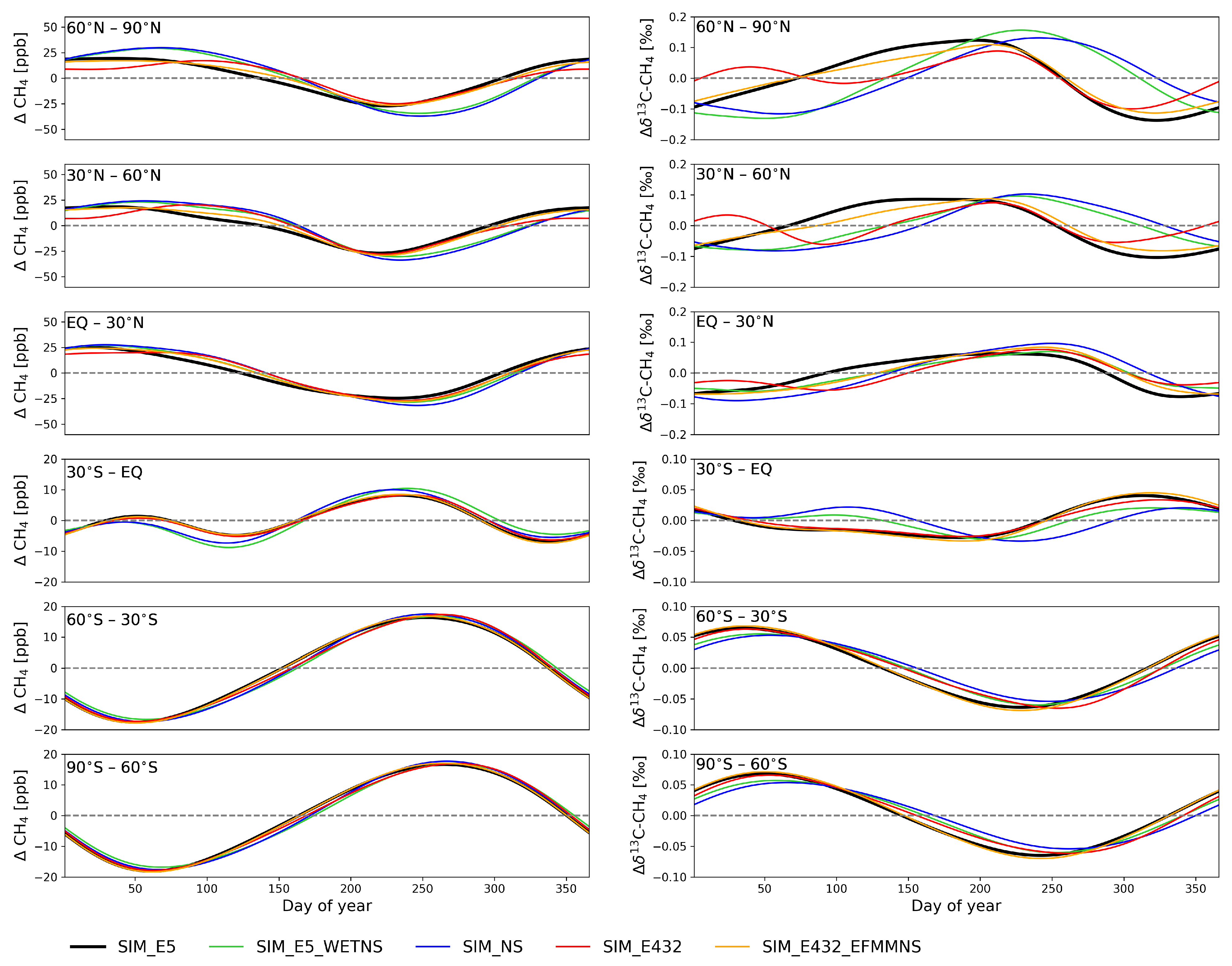
3.1. Zonal Means near the Surface

The de-trended zonal mean atmospheric CH₄ ($\mathsf{\Delta }$CH₄) and ${\delta }^{13}$C ($\mathsf{\Delta }$${\delta }^{13}$C) values from the simulations were compared at 30° latitudinal bands. The trend and smoothed fit were calculated for 2000–2012 from the lowest five layers of the TM5 (up to approximately 850 hPa) based on Thoning et al. [69], and the de-trended smoothed fit was averaged over 2002–2012 to examine the seasonal cycle. We found that it takes approximately two years for the seasonal cycle of the lower atmosphere to stabilize following a change in emission fields from the spin-up (Figure S10). Therefore, to remove the effect of the initial state, the first two years of the forward simulations were omitted from the analysis. In this section, we focus on the seasonal cycle in $\mathsf{\Delta }$${\delta }^{13}$C and its relation to the $\mathsf{\Delta }$CH₄ cycle in Section 3.1.2, as the CH₄ cycle has been discussed extensively in previous studies, e.g., [71,72,73,74].

We acknowledge that the ${\delta }^{13}$C cycles are affected by local sources and can vary spatially at a smaller resolution than 30° latitudinal bands [16,34,35,37,75]. In addition, tropical meteorological dynamics such as the positions of the Intertropical Convergence Zone and the South Pacific Convergence Zone affect the seasonality of CH₄ and ${\delta }^{13}$C, and these variations cannot be distinguished by using 30° latitudinal means [76].

3.1.1. Peak-to-Peak Amplitude and Shape of ${\delta }^{13}$C Seasonal Cycle

Generally, the seasonal cycle of $\mathsf{\Delta }$${\delta }^{13}$C is the reverse of the seasonal cycle of $\mathsf{\Delta }$CH₄, such that ${\delta }^{13}$C has a seasonal minimum in winter and a maximum in summer in the NH, and vice versa for the SH (Figure 2) as shown in, e.g., Allan et al. [34] and Bergamaschi et al. [35]. Seasonal variations in both CH₄ and ${\delta }^{13}$C are larger in the NH than in the SH, mostly because the major emission sources are in the NH. The estimated seasonal cycle amplitudes for $\mathsf{\Delta }$CH₄ and $\mathsf{\Delta }$${\delta }^{13}$C were the largest in the NH Tropics, and at 60° N–90° N, respectively, and the smallest amplitude was found in the SH Tropics (SIM_E5). Those results are consistent with previous studies, e.g., [33,35,36,38]. The seasonality of the emission sources caused the $\mathsf{\Delta }$${\delta }^{13}$C minima to lag approximately 1–3 months from the $\mathsf{\Delta }$CH₄ maxima. This was not seen in the simulation, where the seasonality of emissions was removed (SIM_NS). Despite the differences in the emission seasonality, the $\mathsf{\Delta }$CH₄ seasonal cycle amplitude did not differ significantly between the simulations.

At latitudes north of 30° N, modifying emissions had a pronounced influence on the seasonal cycle of both $\mathsf{\Delta }$CH₄ and $\mathsf{\Delta }$${\delta }^{13}$C (Figure 2). The simulation with constant wetland emissions (SIM_E5_WETNS) had higher wetland emissions from winter to spring, and lower from summer to autumn, compared to the reference simulation (SIM_E5). This led to a higher $\mathsf{\Delta }$CH₄ in spring at latitudes north of 30° N, and a lower one from summer to autumn, compared to the reference simulation (SIM_E5). Wetland CH₄ emissions were strongly depleted (Table 1), which resulted in strong $\mathsf{\Delta }$${\delta }^{13}$C depletion in spring and enrichment in autumn. The minima of $\mathsf{\Delta }$${\delta }^{13}$C in SIM_E5_WETNS were then shifted to the beginning of the year by 69–93 days, and the maxima in autumn were delayed by 29–32 days at the NH, except for the band 30° N–60° N, which was shifted toward autumn by 67 days compared to SIM_E5.

In the NH, the simulation using EDGAR v4.3.2 (SIM_E432) had a clear double peak structure in the $\mathsf{\Delta }$${\delta }^{13}$C, which was not visible in the other simulations. In spring, the $\mathsf{\Delta }$${\delta }^{13}$C was quickly decreased due to high EFMM emissions. When removing the seasonal variations of the EFMM emissions (SIM_E432_EFMMNS), the shape of the seasonal cycle in $\mathsf{\Delta }$${\delta }^{13}$C became closer to SIM_E5. The lower winter EFMM emissions contributed to an increase in $\mathsf{\Delta }$${\delta }^{13}$C at the beginning of the year, i.e., there was a small lag-effect on how emissions affect $\mathsf{\Delta }$${\delta }^{13}$C the cycle.

At low southern latitudes (30° S–EQ), there was a double peak structure in the $\mathsf{\Delta }$CH₄ due to the high wetland emissions in January–March and the high biomass burning emissions in August–October (Figure 1). A double peak structure was also visible in the $\mathsf{\Delta }$${\delta }^{13}$C with the simulation of constant emissions and the simulation of constant wetland emissions (SIM_NS and SIM_E5_WETNS). However, the double peak in the $\mathsf{\Delta }$${\delta }^{13}$C disappeared when seasonal variations of CH₄ were considered (SIM_E5). This is because the ${\delta }^{13}$C was decreased by high wetland emissions in the SH summer and autumn and increased by strong biomass burning emissions in the SH spring. The similar behavior of SIM_NS and SIM_E5_WETNS indicates that wetlands are the largest individual source driving the ${\delta }^{13}$C seasonal cycle, apart from sinks. Biomass burning also affected the seasonality in this region such that when the seasonality of biomass burning was excluded (SIM_NS), the emissions were lower during the peak in August–October and higher during other months, leading to enriched $\mathsf{\Delta }$${\delta }^{13}$C during February–June and depleted $\mathsf{\Delta }$${\delta }^{13}$C during July–November, compared to SIM_E5_WETNS.

At latitudes south of 60° S, the CH₄ emissions are small (Figure 1), so the seasonal cycles of both CH₄ and ${\delta }^{13}$C are primarily determined by the atmospheric sinks. Therefore, at these latitudes, the differences in the simulations were very small.

3.1.2. Phase Ellipses

The seasonal cycle of $\mathsf{\Delta }$${\delta }^{13}$C with respect to the $\mathsf{\Delta }$CH₄ cycle can be examined with a so-called phase ellipse [34,35]. The phase ellipses, where $\mathsf{\Delta }$${\delta }^{13}$C is plotted against $\mathsf{\Delta }$CH₄, contain the same information as the time series (Figure 2), but they provide better visualization of the phase difference between the two. Figure 3 shows phase ellipses from the simulations using different emission fields at 30° latitudinal bands. The length of the major axis of the ellipse represents the amplitude of the seasonal cycle, and eccentricity represents phase differences. In addition, we examined the timing d (DOY) when the shifted correlations ($p_s$) between $\mathsf{\Delta }$CH₄ at a time t and $\mathsf{\Delta }$${\delta }^{13}$C at time $t+d$ are at minimum and maximum. This quantified the differences in the timing of minimum (maximum) in $\mathsf{\Delta }$CH₄ and maximum (minimum) in $\mathsf{\Delta }$${\delta }^{13}$C (Figure S11). If the $\mathsf{\Delta }$${\delta }^{13}$C cycle is a perfect inverse of the $\mathsf{\Delta }$CH₄ cycle, the ellipse becomes a straight line with a negative slope, because when $\mathsf{\Delta }$CH₄ is increasing, $\mathsf{\Delta }$${\delta }^{13}$C is decreasing. Such a case would be when the CH₄ fluxes have no seasonal cycle and only the atmospheric sinks derive the seasonality of the mixing ratios. In that case, the $\mathsf{\Delta }$CH₄ maximum (minimum) occurs simultaneously with the $\mathsf{\Delta }$${\delta }^{13}$C minimum (maximum), and we expect $d_{\min }$ = 0 and $d_{\max }$ = 366/2 = 183.

Note that the rotation with respect to the DOY in the NH is anticlockwise, and that in the SH, it is clockwise (Figure 3). In addition to the phase ellipses, Figure 3 illustrates the theoretical KIE line when only the OH sink is considered [34]. The KIE line slope was calculated according to Allan et al. [34] as $ϵ(1+{\delta }_0)$, where $ϵ$ is (k₁₃/k₁₂)_OH −1, and ${\delta }_0$ is the mean of the smoothed fit 13C divided by the mean of the smoothed fit CH₄ in SIM_NS. Using the KIE of OH resulted in a slope of −0.0023‰ ppb ${}^{-1}$ corresponding to −3.79‰. The corresponding value was obtained by multiplying the slope with the mean of the smoothed fit CH₄.

When the emission seasonality was included (SIM_E5), the ellipses’ eccentricity decreased, and the shape became more like a circle (Figure 3). The anti-correlation became weaker, R² became smaller, and d shifted by −97 days, which was the maximum (Figure S11). The length of the ellipse major axis in SIM_E5 was longer in the NH compared to the SH, because most of the CH₄ sources were located in the NH, and the seasonality of CH₄ emissions are stronger in the NH.

At latitudes north of 30° N, d in SIM_E5 is shifted by approximately −60 days compared to SIM_NS (Figure S11), indicating that the minimum of $\mathsf{\Delta }$${\delta }^{13}$C was 60 days earlier than the maximum of $\mathsf{\Delta }$CH₄. In addition, the phase ellipses in SIM_E5_WETNS were closer to that of SIM_NS than to SIM_E5, indicating again the strong influence of wetland emissions.

The phase ellipses in SIM_E432 at latitudes north of 30° N had a unique shape of a tilted number eight due to the seasonality of EFMM emissions, resulting in the weakest anti-correlation and the smallest R² (Figure 3). The shapes of the SIM_E432_EFMMNS ellipses north of 30° N were closer to those of SIM_E5 compared to SIM_E432. This was expected, as the $\mathsf{\Delta }$${\delta }^{13}$C seasonal cycle is close to that of SIM_E5 (Section 3.1.1).

The irregular shape found in the low SH latitudes (30° S–EQ) was due to high wetland emissions with depleted isotopic signatures in January–March and high biomass burning emissions with an enriched isotopic signature in August–October (Figure 1). As illustrated in Figure 2, the $\mathsf{\Delta }$${\delta }^{13}$C decreased in the beginning of the year until the DOY ≈ 200, while $\mathsf{\Delta }$CH₄ had both increasing and decreasing phases during that time. This creates a zigzag line for DOY ≤ 200. When the emission seasonality was removed (SIM_NS), the phase ellipse was close to a straight line, but the shifted correlations had two maxima at DOY = 117 and 270, with $p_s\approx 0.5$ on these days (Figure S11).

At latitudes south of 30° S, the SIM_E5 phase ellipses’ eccentricities were very high, with a strong anti-correlation compared to those in the NH (Figure 3). This indicates that $\mathsf{\Delta }$CH₄ and $\mathsf{\Delta }$${\delta }^{13}$C were close to perfect inverse phases, i.e., the seasonal cycles were preliminarily driven by the atmospheric sinks and hardly affected by the seasonal cycle of emissions. However, the phase ellipse from SIM_NS does not exactly follow the KIE line, indicating the effect of sinks other than OH, i.e., stratospheric Cl, O(¹D) and soil sinks, and horizontal long-range and vertical transport.

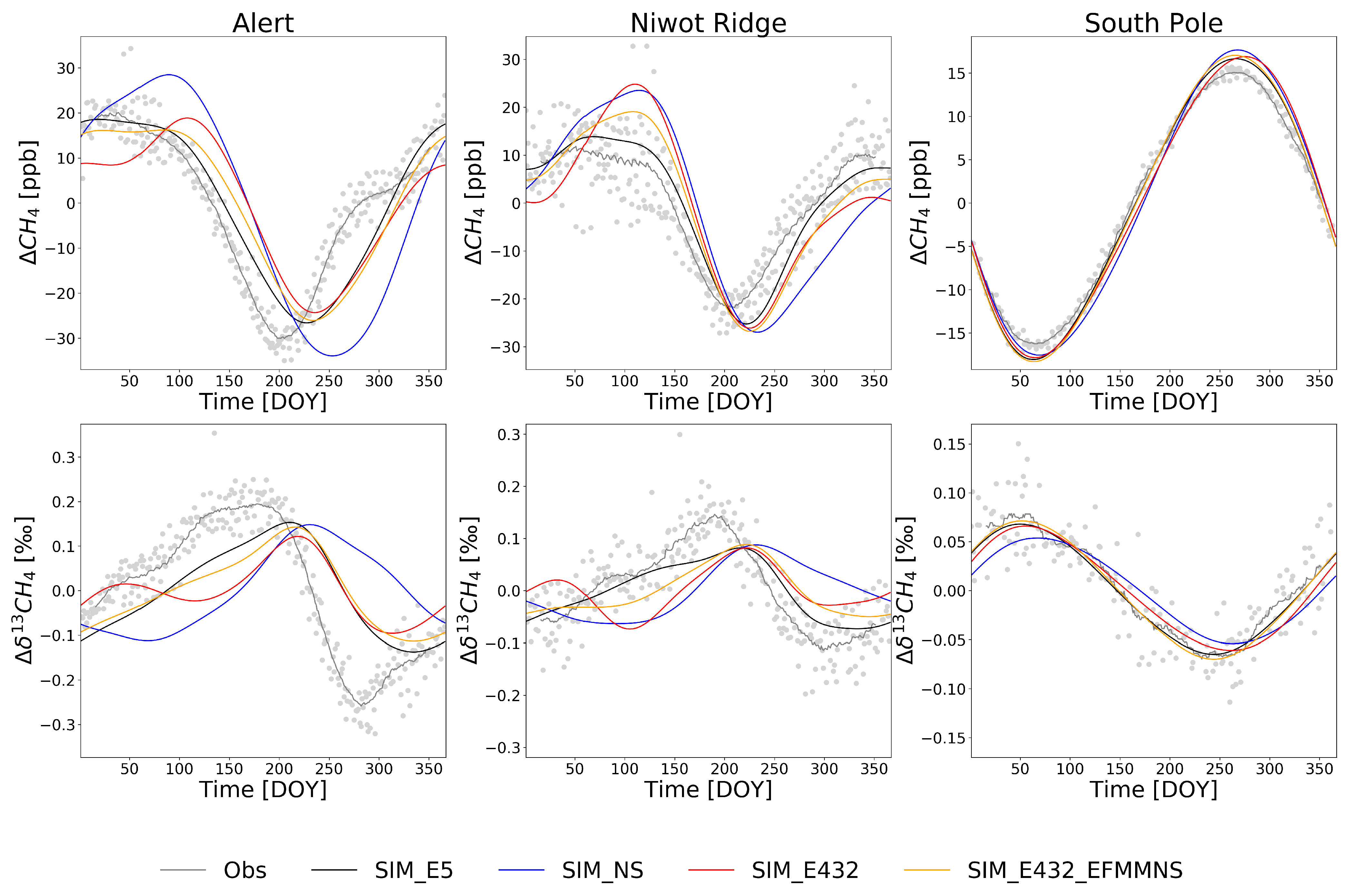
3.2. Comparison to Surface Observations

In this analysis, we focus on the evaluation of SIM_E5, SIM_NS, SIM_E432, and SIM_E432_EFMM to examine which emission cycle best matches the observed seasonal cycle in ${\delta }^{13}$C. The peaks and amplitude of the observations were calculated from 30-day moving averages of the de-trended data because the variations in the observations are high even after the smooth fitting (Figure 4). This section focuses on the results from ALT, NWR, and SPO. The results from other stations are presented in Figures S5–S9 and Tables S3 and S4.

At the SPO station, the modeled $\mathsf{\Delta }$${\delta }^{13}$C followed the shape of the seasonal cycle well (Figure 4), but the modeled seasonal cycle amplitudes were smaller compared to the observations (

Table 5. Observed and modeled amplitudes of Δδ¹³C and ΔCH₄ at Alert (ALT), Niwot Ridge (NWR), and South Pole (SPO) stations.

Species	Station Code	Observation	SIM_E5	SIM_NS	SIM_E432	SIM_E432_EFMMNS
$\mathsf{\Delta }$${\delta }^{13}$C (‰)	ALT	0.45	0.29	0.26	0.22	0.26
	NWR	0.26	0.15	0.15	0.16	0.14
	SPO	0.15	0.13	0.11	0.13	0.14
$\mathsf{\Delta }$CH4 (ppb)	ALT	50.1	45.2	62.4	43.2	42.3
	NWR	33.7	39.1	50.5	50.9	45.9
	SPO	31.3	34.7	35.2	34.7	35.3

). For the $\mathsf{\Delta }$CH₄, the modeled amplitudes were 10.8–12.9% larger than the observations (Table 5). As expected, there were no major differences between the simulations at the SPO, as the site is far from emission sources, except for the SIM_NS simulation where the amplitude of $\mathsf{\Delta }$${\delta }^{13}$C was 27.4% smaller than in the observations (Table 5). A similar feature was seen at the SH sites (Figures S8–S9 and Tables S3–S4).

At ALT (Figure 4), the seasonal amplitude was underestimated in the model by 36–53% (Table 5). This is mainly because the model is not capturing the strong $\mathsf{\Delta }$${\delta }^{13}$C depletion in summer and autumn (see Section 4 for discussions on reasons). This is true also for other northern latitudes sites (north of 55° N, Figures S5–S6 and Tables S3 and S4). At most of those sites, the simulations SIM_E5 and SIM_E432_EFMMNS showed enrichment in $\mathsf{\Delta }$${\delta }^{13}$C from the beginning of the year until the DOY ≈ 200, similar to the observations. However, SIM_E432 showed depletion from the DOY ∼50 to 120 and SIM_NS during the DOY 0 to ∼75. This suggests that the EFMM emission cycle in EDGAR v4.3.2 caused a depletion in spring, as was shown in the zonal mean estimates (see Section 3.1.1). The effect of the CH₄ source seasonality to the ${\delta }^{13}$C was apparent by comparing SIM_NS to other simulations. In addition, the model reached the $\mathsf{\Delta }$${\delta }^{13}$C maximum and minimum ∼20 days later than the observations, and in SIM_NS, the shift is much larger for the minima.

The modeled $\mathsf{\Delta }$CH₄ at ALT had smaller amplitudes than the observations (Table 5), except in SIM_NS where the amplitude was 24% larger due to larger emissions during winter and smaller in summer. The modeled $\mathsf{\Delta }$CH₄ followed the observations well in SIM_E5 and SIM_E432_EFMMNS, while it was smaller than the observations at approximately DOYs <75 in SIM_E432. The observed $\mathsf{\Delta }$CH₄ reached its maximum DOY ≈ 50 in spring, but the model estimated that, in SIM_NS and SIM_E432_EFMMNS, this happened 50–75 days later. The observed $\mathsf{\Delta }$CH₄ reached its minimum at the DOY ≈ 200, but all model estimates were approximately 50 days later. The shape and amplitude of the $\mathsf{\Delta }$CH₄ cycle was closest to the observations in SIM_E5. In general, when the modeled $\mathsf{\Delta }$${\delta }^{13}$C was lower than the observations, the modeled $\mathsf{\Delta }$CH₄ was higher than the observations, except during the DOY ≈ 0–100 in SIM_E5 and SIM_E432_EFMMNS, when $\mathsf{\Delta }$${\delta }^{13}$C was smaller and $\mathsf{\Delta }$CH₄ was lower or close to the observations. The differences between the model estimates and observations may be due to a smaller magnitude of wetland CH₄ emissions (higher values of ${\delta }^{13}$C and a lower magnitude of CH₄) or a smaller magnitude of OH sinks (higher values of ${\delta }^{13}$C). However, increasing wetland CH₄ emissions in summer would cause larger discrepancies in CH₄ abundance in summer–autumn [16], so the magnitude of wetland CH₄ emissions is probably not the only cause. In addition, higher OH concentrations during spring and early summer and lower OH concentrations in autumn could lead to a better match with the observations. Note that changes in the emissions affected the modeled CH₄ and ${\delta }^{13}$C with some lag (see Section 3.1.2), but changes in OH could affect it with a shorter lag time.

At NWR, the modeled amplitude of the $\mathsf{\Delta }$${\delta }^{13}$C was approximately half of the observations (Table 5). All four simulations showed a depletion in summer, ∼50 days later than the observations suggest (Figure 4). This is a general feature at other northern latitude sites (north of 38° N). The depletion in autumn was not as strong as at ALT, and the models followed the depletion better, except in SIM_NS, although the minima were slightly shallower compared to the observations. The observations showed strong summer enrichment of $\mathsf{\Delta }$${\delta }^{13}$C at NWR at the DOY ≈ 200, but none of the simulations could reproduce the peak. Similarly, the summer maxima were underestimated by the simulations at ZEP, SUM, CBA, AZR, WLG, KUM, and MEX (Figures S5–S8). At northern latitude sites (north of 55° N), the discrepancies were high, especially in the simulations using EDGAR v4.3.2 and in simulations without emission seasonality.

The amplitude of the modeled $\mathsf{\Delta }$CH₄ at NWR was 16–51% larger compared with the observations (Table 5). The modeled CH₄ in SIM_E5 reached the maximum approximately at the same time as the observations, but the modeled maximum in SIM_NS, SIM_E432, and SIM_E432_EFMMNS was ∼75 days later than the observed. The timing of the minimum, however, did not differ much: all simulations reached a minimum value ∼25 days later than the observations. All the simulations showed a slight underestimation of $\mathsf{\Delta }$CH₄ in winter. The differences between the modeled and observed $\mathsf{\Delta }$${\delta }^{13}$C in SIM_E5 therefore could be due to the incorrect proportion of biogenic (heavily depleted) to fossil-based (less depleted) emissions sources, especially during the summer. The differences in SIM_E432 in spring suggest that the biogenic EFMM emissions are probably overestimated. However, although the seasonal cycle of EFMM emissions was removed, the spring discrepancies remained (SIM_E432_EFMMNS). In addition, the differences in both $\mathsf{\Delta }$CH₄ and ¹³C in winter suggest an underestimation of biogenic emissions from all simulations.

4. Discussion

4.1. Isotope Signatures

The seasonality of ${\delta }^{13}$C depends on the isotopic signature of the emissions. It is one of the largest uncertainties in the estimation of modeled ${\delta }^{13}$C. Changing the isotopic signature for a few per mill can reduce or increase the ${\delta }^{13}$C seasonal cycle amplitude by 1.5–7 times, and the timing of minima/maxima by 7–130 days at 30° latitudinal bands (Figure S12), which is in line with the study by Ganesan et al. [27]. Although we have used recently published spatial distributions of source signatures where available, there are still large uncertainties. The isotopic source signatures are especially important for emission sources that have large seasonality, such as wetlands, EFMM, rice, and biomass burning. Therefore, the seasonality in the emission is not the only reason for the discrepancies between modeled and observed ${\delta }^{13}$C values.

The isotopic signatures in northern wetlands during autumn could be more negative [77], which could be a reason why our modeled ${\delta }^{13}$C values in high northern latitude sites, e.g., Alert, were overestimated. The isotopic source signatures for manure management and enteric fermentation depend on different factors (e.g., manure type vs. livestock diet) [28,30,78,79], but we applied the same isotopic signature for manure management and enteric fermentation, and CH₄ emissions are summed up as one category. Although such information is not yet available globally, properly distinguishing those sectors could also improve modeled ${\delta }^{13}$C seasonality at NH sites, e.g., at ALT and NWR, even when using EDGAR v4.3.2 emissions. The isotopic source signatures for rice emissions may be less negative depending on cultivation methods [80,81]. This would enrich the modeled ${\delta }^{13}$C value, i.e., less depletion of ${\delta }^{13}$C in spring in the NH from SIM_E432, and higher ${\delta }^{13}$C in summer from SIM_E5.

In addition, we acknowledge that the isotopic source signatures may have seasonal variations. These variations have been reported for biogenic sources, such as wetlands [60,82] and rice cultivation [80,83,84,85]. These sources typically show depletion in ${\delta }^{13}$C when CH₄ emission is high because more ¹²C is consumed (oxidized) by the microbes. This would lead to more depleted modeled ${\delta }^{13}$C in summer due to wetlands and rice (in the case of EDGAR v5.0), and a stronger depletion of ${\delta }^{13}$C in spring in the NH using EDGAR v4.3.2. However, the seasonality may be opposite for ruminants, landfills, and forested wetlands such that ${\delta }^{13}$C is more depleted during cold seasons, e.g., NH winter, than warmer seasons [86,87]. Furthermore, it is known that the ${\delta }^{13}$C signature of biomass burning varies during different phases, e.g., smoldering vs. flaming phases [88]. Therefore, the combined effect on regional levels is uncertain and needs further examination.

Other source signatures, also those from fossil fuels, have temporal changes that could be important to take into account. For example, the coal source signatures vary depending on coal types, depths, coalification processes, the type of mining, and coal rank [89], but only limited measurements and country-level data for coal mining types are available and may be misreported [28], as the coal source signature can also vary within a country [89]. Those would be especially important in analyzing, e.g., long-term trends.

In addition, we acknowledge that the KIE of soil sinks varies among soil types. In this study, we used a value of 1.0177 according to Snover and Quay [56], but the KIE values reported have a range from 1.0173 to 1.025 [56,90,91] depending on soil type. KIE soil sink variations due to temperature and CH₄ concentration due to the variation of a biological KIE [90] are not taken into account in this study. We found that the phase ellipse from the simulation without emission seasonality (SIM_NS) did not follow the theoretical KIE line, and part of that is likely to be driven by the soil sink.

Nevertheless, considering that our results agree well with the observations at the South Pole, we could assume that the currently used isotopic signatures and KIE are correct in a broad sense. A more detailed and a better spatial and temporal distribution of signature values are becoming available, e.g., [92], and using the updated information would improve the agreement with observations and enable us to examine the emission seasonality more accurately.

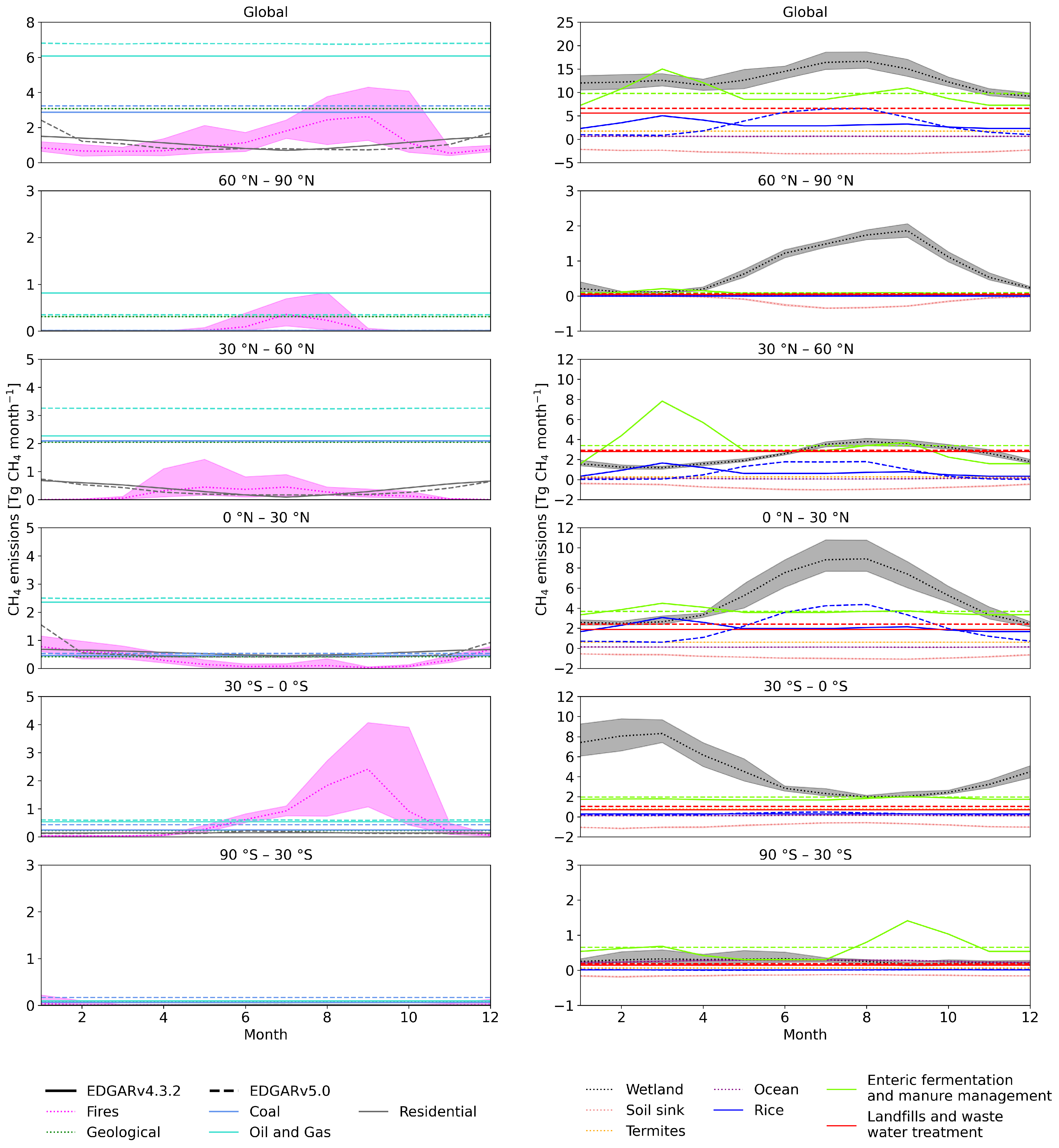
4.2. Seasonal Cycle of CH₄ Emissions

${\delta }^{13}$C measurements could be used to evaluate CH₄ emission magnitude and seasonal cycle, as the changes in ¹³CH₄ emissions of 0.1% could result in ∼1‰ differences in ${\delta }^{13}$C. The wetland CH₄ emissions at high latitudes (north of 50° N) used in this study (LPX-Bern v1.4) had a maximum in September, which agrees with the inversion models, such as Thompson et al. [93] and Bousquet et al. [94]. However, September was later than found in other studies, such as those using process-based models [6,95] or measurements [16,37]. In Aalto et al. [96], it was shown that the main reasons for the late maximum in LPX-Bern v1.4 is the strong precipitation dependence of wetland emissions. In addition, the maximum CH₄ emission at high latitudes in LPX-Bern v1.4 was approximately 3–6 Tg CH₄ month ${}^{-1}$ lower than other model estimates, such as Saunois et al. [3], Warwick et al. [16], Fung et al. [97], and Tenkanen et al. [98]. Other natural emissions, such as those from inland water systems [99], and the effects of the upland soil sink on ¹³C [100] could be reasons for the underestimation of the ${\delta }^{13}$C amplitude at high latitudes in this study. Our comparison to the observations also supports these findings that higher summer emissions and earlier maximum, e.g., in August, would derive a better match to the observations at NHL sites.

The seasonal cycle of CH₄ emissions from the EFMM sector varies considerably between the EDGAR versions. In the NH, the seasonality of enteric fermentation in v5.0 is likely to be more in line with measurements, e.g., [101], but warmer air temperature is likely to enhance manure CH₄ emissions [101,102,103,104,105], contradicting both EDGAR versions. Our results showed better agreement with the observations when using EDGAR v5.0 in the NH, but higher manure emissions in the NH during summer would worsen the agreement unless solid manure, enriched in ¹³C (see Section 4.1), is increased. In the SH, some studies [106,107] show a seasonality of livestock emissions that is more in line with EDGAR v4.3.2. However, our comparison to observations at Baring Head in New Zealand show better agreement using v5.0. Nevertheless, despite the small number of observations, none of the simulations could reproduce a ${\delta }^{13}$C cycle well for the beginning of the year (Figure S9), suggesting that further evaluation and improvements are needed.

CH₄ emissions from rice follow the rice growing calendar [108]. Cao et al. [108] modeled the CH₄ emission from rice with a maximum in July–September north of 20° N, and in December–February in the south of 10° S, while near the equatorial regions, the emissions were high throughout the year, peaking in August. In Zhang et al. [109], global rice CH₄ emissions were also estimated to peak in July–August. Measurements performed during the growing season [83,84] agree with these estimates. CH₄ emissions from rice cultivation provided by EDGAR v5.0 correspond better to these estimates than those from EDGAR v4.3.2.

Other important emissions in the tropics are from fires. The comparison to the observations in the tropics (Ascension Island and Samoa) showed an underestimation of the modeled CH₄ and an overestimation of δ¹³C during September–December. This indicates that higher biogenic emissions are possibly needed, and only changing the magnitude of regional fire emissions would not resolve such discrepancies. Although the seasonality of the GFED is in line with other studies, e.g., [7], the tropical fires are highly heterogeneous both spatially and temporally. Higher temporal-resolution emission estimates could be used (available from the GFED), and detailed spatial distribution could be examined further for a better understanding of the discrepancies found in this study.

4.3. Atmospheric Sinks

OH is the largest CH₄ sink in the atmosphere, and it removes ¹²CH₄ faster than ¹³CH₄. The seasonal cycle of OH is affected by humidity, clouds, temperature, forest fires, and ultraviolet (UV) flux, especially outside the tropics Rohrer and Berresheim [110]. The authors in Lowe et al. [76] speculated that their underestimation of the ${\delta }^{13}$C seasonal cycle amplitude in the tropics may be associated with the OH sink, while the authors in Allan et al. [34] suggested that the overestimation of the CH₄ seasonal cycle in the model is associated with an overestimation of the OH sink by more than 28%. We examined the ${\delta }^{13}$C seasonal cycle by changing the seasonal cycle amplitude of the OH concentrations by ±10%, but the effect on the tropospheric ${\delta }^{13}$C seasonal cycle with respect to CH₄ was insignificant even in the tropics (figure not shown).

Marine boundary-layer (BL) Cl is thought to play a non-negligible role in CH₄ sinks (5–25 Tg yr ${}^{-1}$) [34,38]. An underestimation of tropospheric Cl will likely lead to an underestimation of the ${\delta }^{13}$C seasonal cycle amplitude in the troposphere due to stronger fractionation and assuming that Cl concentration has a similar seasonality to OH [38,111]. In this study, we did not include the tropospheric Cl sink but could nevertheless reproduce the CH₄ and ${\delta }^{13}$C seasonal cycle measured at the South Pole reasonably well. The seasonality at the SPO is mostly driven by atmospheric sinks. A recent study by Gromov et al. [40] suggested that the contribution of the tropospheric Cl sink to atmospheric CH₄ budgets is small. However, it has been shown that marine BL Cl concentration is the highest in the tropics, e.g., [39]. Our model results show that the modeled seasonal cycle did not agree well with the observations in the tropics, and the CH₄ to ${\delta }^{13}$C ratio does not follow the theoretical KIE line even at the southern high latitude, similar to the observation-based study by Allan et al. [34]. They argued that the kinetic isotope fractionation at a site in the SH extratropic requires an CH₄ oxidation pathway by Cl.

Other than the tropospheric sinks, the stratosphere–troposphere exchange also has an effect to some extent [58], so the stratospheric sinks of Cl and O(¹D) could contribute to the tropospheric seasonality. In the stratosphere, the effect of emissions is negligible, and the seasonality is largely driven by the atmospheric sinks. This was true in our simulations as well. The chemical sinks strongly enrich the ${\delta }^{13}$C in the stratosphere. Therefore, the stratospheric air that returns to the troposphere can affect the tropospheric seasonality of $\mathsf{\Delta }$${\delta }^{13}$C in mid and high latitudes.

5. Conclusions

We performed a global analysis of how different CH₄ emission sources influence the ${\delta }^{13}$C seasonal cycle during 2000–2012, using the TM5 atmospheric chemistry transport model. Wetland emissions were found to be the largest individual CH₄ source driving the ${\delta }^{13}$C seasonal cycle, apart from atmospheric sinks. In the Southern Hemisphere Tropics, biomass burning emissions in addition to wetland emissions are an important factor determining the seasonality of $\mathsf{\Delta }$${\delta }^{13}$C. We also found that the effect of sinks other than OH contributes to the $\mathsf{\Delta }$${\delta }^{13}$C cycle in relation to the $\mathsf{\Delta }$CH₄ cycle.

The comparison to global observations indicated that the seasonality of the sinks and emissions in the model are at the right level. However, the modeled $\mathsf{\Delta }$${\delta }^{13}$C seasonal cycle amplitude was underestimated in stations north of 55° N. This may be due to an underestimation of wetland CH₄ emissions in the northern high latitudes in summer, although other factors, e.g., the timing of wetland emission peaks, the seasonal cycle of OH, and isotopic signatures, could also affect the simulated seasonal cycles. The results also suggested that the seasonal cycle of enteric fermentation and manure management (EFMM) emissions in EDGAR v4.3.2 needs to be revised, and the model estimates using EDGAR v5.0 are in better agreement with the observations.

Here, we have focused on the effects of emissions and their source signatures on the simulated seasonal cycle of ${\delta }^{13}$C. The seasonality of anthropogenic emissions in a regional context, especially for the biogenic components, requires further research. Wetland and fire emissions have been intensively studied previously, but uncertainty in regional seasonality still exists. There is an increasing number of studies examining the spatial and temporal distributions of emission signatures, but further research at regional to global scales is needed to examine changes of ${\delta }^{13}$C. In addition, the tropospheric cycles are affected by a stratosphere–troposphere exchange, and this calls for further studies.

In this study, we did not examine the interannual variability of the modeled δ¹³ seasonal cycle. However, changes and exceptional years could be detected and examined further in relation to emission patterns in future studies. Furthermore, a step forward to better understand the different source contributions would be to build an atmospheric inversion and will be the scope of our next study.

References

1. The Core Writing Team; Rajendra, K.P.; Leo, M. (Eds.) IPCC, 2014: Climate Change 2014: Synthesis Report. Contribution of Working Groups I, II and III to the Fifth Assessment Report of the Intergovernmental Panel on Climate Change; Intergovernmental Panel on Climate Change: Geneva, Switzerland, 2015; p. 87. Available online: https://www.ipcc.ch/site/assets/uploads/2018/02/AR5_SYR_FINAL_Front_matters.pdf (accessed on 20 March 2022).
2. Hartmann, D.; Klein Tank, A.; Rusticucci, M.; Alexander, L.; Brönnimann, S.; Charabi, Y.; Dentener, F.; Dlugokencky, E.; Easterling, D.; Kaplan, A.; et al. Observations: Atmosphere and Surface. In Climate Change 2013: The Physical Science Basis. Contribution of Working Group I to the Fifth Assessment Report of the Intergovernmental Panel on Climate Change; Stocker, T., Qin, D., Plattner, G.K., Tignor, M., Allen, S., Boschung, J., Nauels, A., Xia, Y., Bex, V., Midgley, P., Eds.; Cambridge University Press: Cambridge, UK; New York, NY, USA, 2013; Book Section 2; pp. 159–254. [Google Scholar] [CrossRef] [Green Version]
3. Saunois, M.; Stavert, A.R.; Poulter, B.; Bousquet, P.; Canadell, J.G.; Jackson, R.B.; Raymond, P.A.; Dlugokencky, E.J.; Houweling, S.; Patra, P.K.; et al. The Global Methane Budget 2000–2017; Earth System Science Data, Copernicus Publications: Göttingen, Germany, 2020; Volume 12, pp. 1561–1623. [Google Scholar] [CrossRef]
4. Crippa, M.; Solazzo, E.; Huang, G.; Guizzardi, D.; Koffi, E.; Muntean, M.; Schieberle, C.; Friedrich, R.; Janssens-Maenhout, G. High resolution temporal profiles in the Emissions Database for Global Atmospheric Research. Sci. Data 2020, 7, 121. [Google Scholar] [CrossRef] [PubMed]
5. Bergamaschi, P.; Karstens, U.; Manning, A.J.; Saunois, M.; Tsuruta, A.; Berchet, A.; Vermeulen, A.T.; Arnold, T.; Janssens-Maenhout, G.; Hammer, S.; et al. Inverse modelling of European CH4 emissions during 2006–2012 using different inverse models and reassessed atmospheric observations. Atmos. Chem. Phys. 2018, 18, 901–920. [Google Scholar] [CrossRef] [Green Version]
6. Bloom, A.A.; Bowman, K.W.; Lee, M.; Turner, A.J.; Schroeder, R.; Worden, J.R.; Weidner, R.; McDonald, K.C.; Jacob, D.J. A global wetland methane emissions and uncertainty dataset for atmospheric chemical transport models (WetCHARTs version 1.0). Geosci. Model Dev. 2017, 10, 2141–2156. [Google Scholar] [CrossRef] [Green Version]
7. Basso, L.S.; Gatti, L.V.; Gloor, M.; Miller, J.B.; Domingues, L.G.; Correia, C.S.C.; Borges, V.F. Seasonality and interannual variability of CH4 fluxes from the eastern Amazon Basin inferred from atmospheric mole fraction profiles. J. Geophys. Res. Atmos. 2016, 121, 168–184. [Google Scholar] [CrossRef] [PubMed]
8. Giglio, L.; Randerson, J.T.; van der Werf, G.R. Analysis of daily, monthly, and annual burned area using the fourth-generation global fire emissions database (GFED4). J. Geophys. Res. Biogeosci. 2013, 118, 317–328. [Google Scholar] [CrossRef] [Green Version]
9. Kuze, A.; Kikuchi, N.; Kataoka, F.; Suto, H.; Shiomi, K.; Kondo, Y. Detection of Methane Emission from a Local Source Using GOSAT Target Observations. Remote. Sens. 2020, 12, 267. [Google Scholar] [CrossRef] [Green Version]
10. Pandey, S.; Gautam, R.; Houweling, S.; van der Gon, H.D.; Sadavarte, P.; Borsdorff, T.; Hasekamp, O.; Landgraf, J.; Tol, P.; van Kempen, T.; et al. Satellite observations reveal extreme methane leakage from a natural gas well blowout. Proc. Natl. Acad. Sci. USA 2019, 116, 26376–26381. [Google Scholar] [CrossRef]
11. Delwiche, K.B.; Knox, S.H.; Malhotra, A.; Fluet-Chouinard, E.; McNicol, G.; Feron, S.; Ouyang, Z.; Papale, D.; Trotta, C.; Canfora, E.; et al. FLUXNET-CH4: A global, multi-ecosystem dataset and analysis of methane seasonality from freshwater wetlands. Earth Syst. Sci. Data Discuss. 2021, 13, 3607–3689. [Google Scholar] [CrossRef]
12. Villarreal, S.; Vargas, R. Representativeness of FLUXNET Sites Across Latin America. J. Geophys. Res. Biogeosci. 2021, 126, e2020JG006090. [Google Scholar] [CrossRef]
13. Parker, R.J.; Wilson, C.; Bloom, A.A.; Comyn-Platt, E.; Hayman, G.; McNorton, J.; Boesch, H.; Chipperfield, M.P. Exploring constraints on a wetland methane emission ensemble (WetCHARTs) using GOSAT observations. Biogeosciences 2020, 17, 5669–5691. [Google Scholar] [CrossRef]
14. Xu, X.; Riley, W.J.; Koven, C.D.; Billesbach, D.P.; Chang, R.Y.W.; Commane, R.; Euskirchen, E.S.; Hartery, S.; Harazono, Y.; Iwata, H.; et al. A multi-scale comparison of modeled and observed seasonal methane emissions in northern wetlands. Biogeosciences 2016, 13, 5043–5056. [Google Scholar] [CrossRef] [Green Version]
15. Zhang, Y.; Jacob, D.J.; Lu, X.; Maasakkers, J.D.; Scarpelli, T.R.; Sheng, J.X.; Shen, L.; Qu, Z.; Sulprizio, M.P.; Chang, J.; et al. Attribution of the accelerating increase in atmospheric methane during 2010–2018 by inverse analysis of GOSAT observations. Atmos. Chem. Phys. 2021, 21, 3643–3666. [Google Scholar] [CrossRef]
16. Warwick, N.J.; Cain, M.L.; Fisher, R.; France, J.L.; Lowry, D.; Michel, S.E.; Nisbet, E.G.; Vaughn, B.H.; White, J.W.C.; Pyle, J.A. Using δ13C-CH4 and δD-CH4 to constrain Arctic methane emissions. Atmos. Chem. Phys. 2016, 16, 14891–14908. [Google Scholar] [CrossRef] [Green Version]
17. Tsuruta, A.; Aalto, T.; Backman, L.; Krol, M.C.; Peters, W.; Lienert, S.; Joos, F.; Miller, P.A.; Zhang, W.; Laurila, T.; et al. Methane budget estimates in Finland from the CarbonTracker Europe-CH4 data assimilation system. Tellus B Chem. Phys. Meteorol. 2019, 71, 1565030. [Google Scholar] [CrossRef] [Green Version]
18. Yan, X.; Akiyama, H.; Yagi, K.; Akimoto, H. Global estimations of the inventory and mitigation potential of methane emissions from rice cultivation conducted using the 2006 Intergovernmental Panel on Climate Change Guidelines. Glob. Biogeochem. Cycles 2009, 23, GB2002. [Google Scholar] [CrossRef]
19. Elsgaard, L.; Olsen, A.B.; Petersen, S.O. Temperature response of methane production in liquid manures and co-digestates. Sci. Total Environ. 2016, 539, 78–84. [Google Scholar] [CrossRef]
20. Nisbet, E.G.; Dlugokencky, E.J.; Manning, M.R.; Lowry, D.; Fisher, R.E.; France, J.L.; Michel, S.E.; Miller, J.B.; White, J.W.C.; Vaughn, B.; et al. Rising atmospheric methane: 2007–2014 growth and isotopic shift. Glob. Biogeochem. Cycles 2016, 30, 1356–1370. [Google Scholar] [CrossRef] [Green Version]
21. Sherwood, O.A.; Schwietzke, S.; Arling, V.A.; Etiope, G. Global Inventory of Gas Geochemistry Data from Fossil Fuel, Microbial and Burning Sources, version 2017. Earth Syst. Sci. Data 2017, 9, 639–656. [Google Scholar] [CrossRef] [Green Version]
22. Schwietzke, S.; Sherwood, O.A.; Bruhwiler, L.M.P.; Miller, J.B.; Etiope, G.; Dlugokencky, E.J.; Michel, S.E.; Arling, V.A.; Vaughn, B.H.; White, J.W.C.; et al. Upward revision of global fossil fuel methane emissions based on isotope database. Nature 2016, 538, 88–91. [Google Scholar] [CrossRef]
23. Thompson, R.L.; Nisbet, E.G.; Pisso, I.; Stohl, A.; Blake, D.; Dlugokencky, E.J.; Helmig, D.; White, J.W.C. Variability in Atmospheric Methane From Fossil Fuel and Microbial Sources Over the Last Three Decades. Geophys. Res. Lett. 2018, 45, 11499–11508. [Google Scholar] [CrossRef] [Green Version]
24. Monteil, G.; Houweling, S.; Dlugockenky, E.J.; Maenhout, G.; Vaughn, B.H.; White, J.W.C.; Rockmann, T. Interpreting methane variations in the past two decades using measurements of CH4 mixing ratio and isotopic composition. Atmos. Chem. Phys. 2011, 11, 9141–9153. [Google Scholar] [CrossRef] [Green Version]
25. Lan, X.; Basu, S.; Schwietzke, S.; Bruhwiler, L.M.P.; Dlugokencky, E.J.; Michel, S.E.; Sherwood, O.A.; Tans, P.P.; Thoning, K.; Etiope, G.; et al. Improved Constraints on Global Methane Emissions and Sinks Using δ13C-CH4. Glob. Biogeochem. Cycles 2021, 35, e2021GB007000. [Google Scholar] [CrossRef]
26. Houweling, S.; Krol, M.; Bergamaschi, P.; Frankenberg, C.; Dlugokencky, E.J.; Morino, I.; Notholt, J.; Sherlock, V.; Wunch, D.; Beck, V.; et al. A multi-year methane inversion using SCIAMACHY, accounting for systematic errors using TCCON measurements. Atmos. Chem. Phys. 2014, 14, 3991–4012. [Google Scholar] [CrossRef] [Green Version]
27. Ganesan, A.L.; Stell, A.C.; Gedney, N.; Comyn-Platt, E.; Hayman, G.; Rigby, M.; Poulter, B.; Hornibrook, E.R.C. Spatially Resolved Isotopic Source Signatures of Wetland Methane Emissions. Geophys. Res. Lett. 2018, 45, 3737–3745. [Google Scholar] [CrossRef]
28. Feinberg, A.I.; Coulon, A.; Stenke, A.; Schwietzke, S.; Peter, T. Isotopic source signatures: Impact of regional variability on the δ13CH4 trend and spatial distribution. Atmos. Environ. 2018, 174, 99–111. [Google Scholar] [CrossRef]
29. Etiope, G.; Ciotoli, G.; Schwietzke, S.; Schoell, M. Gridded maps of geological methane emissions and their isotopic signature. Earth Syst. Sci. Data 2019, 11, 1–22. [Google Scholar] [CrossRef] [Green Version]
30. Brownlow, R.; Lowry, D.; Fisher, R.E.; France, J.L.; Lanoisellé, M.; White, B.; Wooster, M.J.; Zhang, T.; Nisbet, E.G. Isotopic Ratios of Tropical Methane Emissions by Atmospheric Measurement: Tropical Methane δ13 C Source Signatures. Glob. Biogeochem. Cycles 2017, 31, 1408–1419. [Google Scholar] [CrossRef] [Green Version]
31. Saueressig, G.; Crowley, J.N.; Bergamaschi, P.; Brühl, C.; Brenninkmeijer, C.A.M.; Fischer, H. Carbon 13 and D kinetic isotope effects in the reactions of CH4 with O(1D) and OH: New laboratory measurements and their implications for the isotopic composition of stratospheric methane. J. Geophys. Res. Atmos. 2001, 106, 23127–23138. [Google Scholar] [CrossRef]
32. Cantrell, C.A.; Shetter, R.E.; McDaniel, A.H.; Calvert, J.G.; Davidson, J.A.; Lowe, D.C.; Tyler, S.C.; Cicerone, R.J.; Greenberg, J.P. Carbon kinetic isotope effect in the oxidation of methane by the hydroxyl radical. J. Geophys. Res. Atmos. 1990, 95, 22455–22462. [Google Scholar] [CrossRef] [Green Version]
33. Bergamaschi, P.; Brühl, C.; Brenninkmeijer, C.a.M.; Saueressig, G.; Crowley, J.N.; Grooß, J.U.; Fischer, H.; Crutzen, P.J. Implications of the large carbon kinetic isotope effect in the reaction CH4 + Cl for the 13C/12C ratio of stratospheric CH4. Geophys. Res. Lett. 1996, 23, 2227–2230. [Google Scholar] [CrossRef]
34. Allan, W.; Manning, M.R.; Lassey, K.R.; Lowe, D.C.; Gomez, A.J. Modeling the variation of δ13C in atmospheric methane: Phase ellipses and the kinetic isotope effect. Glob. Biogeochem. Cycles 2001, 15, 467–481. [Google Scholar] [CrossRef]
35. Bergamaschi, P.; Bräunlich, M.; Marik, T.; Brenninkmeijer, C.A.M. Measurements of the carbon and hydrogen isotopes of atmospheric methane at Izaña, Tenerife: Seasonal cycles and synoptic-scale variations. J. Geophys. Res. Atmos. 2000, 105, 14531–14546. [Google Scholar] [CrossRef]
36. Tyler, S.C.; Rice, A.L.; Ajie, H.O. Stable isotope ratios in atmospheric CH4: Implications for seasonal sources and sinks. J. Geophys. Res. Atmos. 2007, 112, D03303. [Google Scholar] [CrossRef]
37. Fujita, R.; Morimoto, S.; Umezawa, T.; Ishijima, K.; Patra, P.K.; Worthy, D.E.J.; Goto, D.; Aoki, S.; Nakazawa, T. Temporal Variations of the Mole Fraction, Carbon, and Hydrogen Isotope Ratios of Atmospheric Methane in the Hudson Bay Lowlands, Canada. J. Geophys. Res. Atmos. 2018, 123, 4695–4711. [Google Scholar] [CrossRef]
38. Allan, W.; Struthers, H.; Lowe, D.C. Methane carbon isotope effects caused by atomic chlorine in the marine boundary layer: Global model results compared with Southern Hemisphere measurements. J. Geophys. Res. Atmos. 2007, 112, D04306. [Google Scholar] [CrossRef]
39. Hossaini, R.; Chipperfield, M.P.; Saiz-Lopez, A.; Fernandez, R.; Monks, S.; Feng, W.; Brauer, P.; Glasow, R.v. A global model of tropospheric chlorine chemistry: Organic versus inorganic sources and impact on methane oxidation. J. Geophys. Res. Atmos. 2016, 121, 14271–14297. [Google Scholar] [CrossRef] [Green Version]
40. Gromov, S.; Brenninkmeijer, C.A.M.; Jöckel, P. A very limited role of tropospheric chlorine as a sink of the greenhouse gas methane. Atmos. Chem. Phys. 2018, 18, 9831–9843. [Google Scholar] [CrossRef] [Green Version]
41. Heimann, M. Technical Report No.10: The Global Atmospheric Tracer Model TM2 Technical Report/Deutsches Klimarechenzentrum, Modellbetreuungsgruppe. Hamburg, Germany. October 1996. Available online: https://pure.mpg.de/rest/items/item_3337960_3/component/file_3337962/content (accessed on 20 March 2012).
42. Krol, M.; Houweling, S.; Bregman, B.; Broek, M.v.d.; Segers, A.; Velthoven, P.v.; Peters, W.; Dentener, F.; Bergamaschi, P. The two-way nested global chemistry-transport zoom model TM5: Algorithm and applications. Atmos. Chem. Phys. 2005, 5, 417–432. [Google Scholar] [CrossRef] [Green Version]
43. Huijnen, V.; Williams, J.; van Weele, M.; van Noije, T.; Krol, M.; Dentener, F.; Segers, A.; Houweling, S.; Peters, W.; de Laat, J.; et al. The global chemistry transport model TM5: Description and evaluation of the tropospheric chemistry version 3.0. Geosci. Model Dev. 2010, 3, 445–473. [Google Scholar] [CrossRef] [Green Version]
44. Janssens-Maenhout, G.; Crippa, M.; Guizzardi, D.; Muntean, M.; Schaaf, E.; Dentener, F.; Bergamaschi, P.; Pagliari, V.; Olivier, J.G.J.; Peters, J.A.H.W.; et al. EDGAR v4.3.2 Global Atlas of the three major greenhouse gas emissions for the period 1970–2012. Earth Syst. Sci. Data 2019, 11, 959–1002. [Google Scholar] [CrossRef] [Green Version]
45. Tsuruta, A.; Aalto, T.; Backman, L.; Hakkarainen, J.; Laan-Luijkx, I.T.v.d.; Krol, M.C.; Spahni, R.; Houweling, S.; Laine, M.; Dlugokencky, E.; et al. Global methane emission estimates for 2000–2012 from CarbonTracker Europe-CH4 v1.0. Geosci. Model Dev. 2017, 10, 1261–1289. [Google Scholar] [CrossRef] [Green Version]
46. Gregory, D.; Morcrette, J.J.; Jakob, C.; Beljaars, A.C.M.; Stockdale, T. Revision of convection, radiation and cloud schemes in the ECMWF integrated forecasting system. Q.J.R. Meteorol. Soc. 2000, 126, 1685–1710. [Google Scholar] [CrossRef]
47. de Laeter, J.R.; Böhlke, J.K.; Bièvre, P.D.; Hidaka, H.; Peiser, H.S.; Rosman, K.J.R.; Taylor, P.D.P. Atomic weights of the elements. Review 2000 (IUPAC Technical Report). De Gruyter Sect. Pure Appl. Chem. 2003, 75, 683–800. [Google Scholar] [CrossRef]
48. Spivakovsky, C.M.; Logan, J.A.; Montzka, S.A.; Balkanski, Y.J.; Foreman-Fowler, M.; Jones, D.B.A.; Horowitz, L.W.; Fusco, A.C.; Brenninkmeijer, C.a.M.; Prather, M.J.; et al. Three-dimensional climatological distribution of tropospheric OH: Update and evaluation. J. Geophys. Res. Atmos. 2000, 105, 8931–8980. [Google Scholar] [CrossRef]
49. Jöckel, P.; Tost, H.; Pozzer, A.; Brühl, C.; Buchholz, J.; Ganzeveld, L.; Hoor, P.; Kerkweg, A.; Lawrence, M.G.; Sander, R.; et al. The atmospheric chemistry general circulation model ECHAM5/MESSy1: Consistent simulation of ozone from the surface to the mesosphere. ATmospheric Chem. Phys. 2006, 6, 5067–5104. [Google Scholar] [CrossRef] [Green Version]
50. Schaefer, H.; Fletcher, S.E.M.; Veidt, C.; Lassey, K.R.; Brailsford, G.W.; Bromley, T.M.; Dlugokencky, E.J.; Michel, S.E.; Miller, J.B.; Levin, I.; et al. A 21st-century shift from fossil-fuel to biogenic methane emissions indicated by 13CH4. Science 2016, 352, 80–84. [Google Scholar] [CrossRef]
51. Montzka, S.A.; Krol, M.; Dlugokencky, E.; Hall, B.; Jöckel, P.; Lelieveld, J. Small Interannual Variability of Global Atmospheric Hydroxyl. Science 2011, 331, 67–69. [Google Scholar] [CrossRef] [Green Version]
52. Lelieveld, J.; Gromov, S.; Pozzer, A.; Taraborrelli, D. Global tropospheric hydroxyl distribution, budget and reactivity. Atmos. Chem. Phys. 2016, 16, 12477–12493. [Google Scholar] [CrossRef] [Green Version]
53. Crowley, J.N.; Saueressig, G.; Bergamaschi, P.; Fischer, H.; Harris, G.W. Carbon kinetic isotope effect in the reaction CH4+Cl: A relative rate study using FTIR spectroscopy. Chem. Phys. Lett. 1999, 303, 268–274. [Google Scholar] [CrossRef] [Green Version]
54. Spahni, R.; Wania, R.; Neef, L.; van Weele, M.; Pison, I.; Bousquet, P.; Frankenberg, C.; Foster, P.N.; Joos, F.; Prentice, I.C.; et al. Constraining global methane emissions and uptake by ecosystems. Biogeosciences 2011, 8, 1643–1665. [Google Scholar] [CrossRef] [Green Version]
55. Lienert, S.; Joos, F. A Bayesian ensemble data assimilation to constrain model parameters and land-use carbon emissions. Biogeosciences 2018, 15, 2909–2930. [Google Scholar] [CrossRef] [Green Version]
56. Snover, A.K.; Quay, P.D. Hydrogen and carbon kinetic isotope effects during soil uptake of atmospheric methane. Glob. Biogeochem. Cycles 2000, 14, 25–39. [Google Scholar] [CrossRef]
57. Röckmann, T.; Brass, M.; Borchers, R.; Engel, A. The isotopic composition of methane in the stratosphere: High-altitude balloon sample measurements. Atmos. Chem. Phys. 2011, 11, 13287–13304. [Google Scholar] [CrossRef] [Green Version]
58. Wang, J.S.; McElroy, M.B.; Spivakovsky, C.M.; Jones, D.B.A. On the contribution of anthropogenic Cl to the increase in δ13C of atmospheric methane. Glob. Biogeochem. Cycles 2002, 16, 20-1–20-11. [Google Scholar] [CrossRef]
59. Houghton, J.; Meira Filho, L.; Lim, K.; Trennton, I.; Mamaty, I.; Bonduki, Y.; Griggs, D.; Callander, B. Revised 1996 IPCC Guidelines for National Greenhouse Gas Inventories; Intergovernmental Panel on Climate Change, Meteorological Office: Bracknell, UK, 1997; Volumes 1–3.
60. Fisher, R.E.; France, J.L.; Lowry, D.; Lanoisellé, M.; Brownlow, R.; Pyle, J.A.; Cain, M.; Warwick, N.; Skiba, U.M.; Drewer, J.; et al. Measurement of the 13C isotopic signature of methane emissions from northern European wetlands. Glob. Biogeochem. Cycles 2017, 31, 605–623. [Google Scholar] [CrossRef] [Green Version]
61. Lambert, G.; Schmidt, S. Reevaluation of the oceanic flux of methane: Uncertainties and long term variations. Chemosphere 1993, 26, 579–589. [Google Scholar] [CrossRef]
62. Dee, D.P.; Uppala, S.M.; Simmons, A.J.; Berrisford, P.; Poli, P.; Kobayashi, S.; Andrae, U.; Balmaseda, M.A.; Balsamo, G.; Bauer, P.; et al. The ERA-Interim reanalysis: Configuration and performance of the data assimilation system. Q. J. R. Meteorol. Soc. 2011, 137, 553–597. [Google Scholar] [CrossRef]
63. Ito, A.; Inatomi, M. Use of a process-based model for assessing the methane budgets of global terrestrial ecosystems and evaluation of uncertainty. Biogeosciences 2012, 9, 759–773. [Google Scholar] [CrossRef] [Green Version]
64. Hmiel, B.; Petrenko, V.V.; Dyonisius, M.N.; Buizert, C.; Smith, A.M.; Place, P.F.; Harth, C.; Beaudette, R.; Hua, Q.; Yang, B.; et al. Preindustrial 14 CH4 indicates greater anthropogenic fossil CH4 emissions. Nature 2020, 578, 409–412. [Google Scholar] [CrossRef]
65. Still, C.J.; Berry, J.A.; Collatz, G.J.; DeFries, R.S. Global distribution of C3 and C4 vegetation: Carbon cycle implications. Glob. Biogeochem. Cycles 2003, 17, 6–1–6–14. [Google Scholar] [CrossRef]
66. Sherwood, O.; Schwietzke, S.; Arling, V.; Etiope, G. Methane δ13C Source Signature Measurements for Improved Atmospheric. 2016. Available online: http://www.esrl.noaa.gov/gmd/ccgg/d13C-src-inv/ (accessed on 23 May 2022).
67. Guidelines for the Measurement of Methane and Nitrous Oxide and their Quality Assurance; WMO/TD-No. 1478, GAW Report No. 185; World Meteorological Organization: Geneva, Switzerland, 2009.
68. Miller, J.B.; Mack, K.A.; Dissly, R.; White, J.W.C.; Dlugokencky, E.J.; Tans, P.P. Development of analytical methods and measurements of 13C/12C in atmospheric CH4 from the NOAA Climate Monitoring and Diagnostics Laboratory Global Air Sampling Network. J. Geophys. Res. Atmos. 2002, 107, ACH 11-1–ACH 11-15. [Google Scholar] [CrossRef]
69. Thoning, K.W.; Tans, P.P.; Komhyr, W.D. Atmospheric carbon dioxide at Mauna Loa Observatory: 2. Analysis of the NOAA GMCC data, 1974–1985. J. Geophys. Res. Atmos. 1989, 94, 8549–8565. [Google Scholar] [CrossRef]
70. Nisbet, E.G.; Manning, M.R.; Dlugokencky, E.J.; Fisher, R.E.; Lowry, D.; Michel, S.E.; Myhre, C.L.; Platt, S.M.; Allen, G.; Bousquet, P.; et al. Very Strong Atmospheric Methane Growth in the 4 Years 2014–2017: Implications for the Paris Agreement. Glob. Biogeochem. Cycles 2019, 33, 318–342. [Google Scholar] [CrossRef]
71. Dlugokencky, E.; Masarie, K.; Tans, P.; Conway, T.; Xiong, X. Is the amplitude of the methane seasonal cycle changing? Atmos. Environ. 1997, 31, 21–26. [Google Scholar] [CrossRef]
72. Javadinejad, S.; Eslamian, S.; Ostad-Ali-Askari, K. Investigation of monthly and seasonal changes of methane gas with respect to climate change using satellite data. Appl. Water Sci. 2019, 9, 180. [Google Scholar] [CrossRef] [Green Version]
73. Kivimäki, E.; Lindqvist, H.; Hakkarainen, J.; Laine, M.; Sussmann, R.; Tsuruta, A.; Detmers, R.; Deutscher, N.M.; Dlugokencky, E.J.; Hase, F.; et al. Evaluation and Analysis of the Seasonal Cycle and Variability of the Trend from GOSAT Methane Retrievals. Remote Sens. 2019, 11, 882. [Google Scholar] [CrossRef] [Green Version]
74. Khalil, M.a.K.; Rasmussen, R.A. Sources, sinks, and seasonal cycles of atmospheric methane. J. Geophys. Res. Ocean. 1983, 88, 5131–5144. [Google Scholar] [CrossRef]
75. Hein, R.; Crutzen, P.J.; Heimann, M. An inverse modeling approach to investigate the global atmospheric methane cycle. Glob. Biogeochem. Cycles 1997, 11, 43–76. [Google Scholar] [CrossRef]
76. Lowe, D.C.; Koshy, K.; Bromley, T.; Allan, W.; Struthers, H.; Mani, F.; Maata, M. Seasonal cycles of mixing ratio and 13C in atmospheric methane at Suva, Fiji. J. Geophys. Res. Atmos. 2004, 109, D23308. [Google Scholar] [CrossRef]
77. Hornibrook, E.R.C. The Stable Carbon Isotope Composition of Methane Produced and Emitted from Northern Peatlands. In Carbon Cycling in Northern Peatlands; American Geophysical Union (AGU): Washington, DC, USA, 2009; pp. 187–203. [Google Scholar] [CrossRef]
78. Chang, J.; Peng, S.; Ciais, P.; Saunois, M.; Dangal, S.R.S.; Herrero, M.; Havlík, P.; Tian, H.; Bousquet, P. Revisiting enteric methane emissions from domestic ruminants and their δ 13 C CH4 source signature. Nat. Commun. 2019, 10, 3420. [Google Scholar] [CrossRef]
79. Levin, I.; Bergamaschi, P.; Dörr, H.; Trapp, D. Stable isotopic signature of methane from major sources in Germany. Chemosphere 1993, 26, 161–177. [Google Scholar] [CrossRef]
80. Zhang, G.; Ma, J.; Yang, Y.; Yu, H.; Shi, Y.; Xu, H. Variations of Stable Carbon Isotopes of CH4 Emission from Three Typical Rice Fields in China. Pedosphere 2017, 27, 52–64. [Google Scholar] [CrossRef]
81. France, J.L.; Fisher, R.E.; Lowry, D.; Allen, G.; Andrade, M.F.; Bauguitte, S.J.B.; Bower, K.; Broderick, T.J.; Daly, M.C.; Forster, G.; et al. δ13C methane source signatures from tropical wetland and rice field emissions. Philos. Trans. R. Soc. A Math. Phys. Eng. Sci. 2022, 380, 20200449. [Google Scholar] [CrossRef]
82. Sriskantharajah, S.; Fisher, R.E.; Lowry, D.; Aalto, T.; Hatakka, J.; Aurela, M.; Laurila, T.; Lohila, A.; Kuitunen, E.; Nisbet, E.G. Stable carbon isotope signatures of methane from a Finnish subarctic wetland. Tellus B Chem. Phys. Meteorol. 2012, 64, 18818. [Google Scholar] [CrossRef]
83. Tyler, S.C.; Brailsford, G.W.; Yagi, K.; Minami, K.; Cicerone, R.J. Seasonal variations in methane flux and δl3CH4 values for rice paddies in Japan and their implications. Glob. Biogeochem. Cycles 1994, 8, 1–12. [Google Scholar] [CrossRef]
84. Bergamaschi, P. Seasonal variations of stable hydrogen and carbon isotope ratios in methane from a Chinese rice paddy. J. Geophys. Res. Atmos. 1997, 102, 25383–25393. [Google Scholar] [CrossRef]
85. Marik, T.; Fischer, H.; Conen, F.; Smith, K. Seasonal variations in stable carbon and hydrogen isotope ratios in methane from rice fields. Glob. Biogeochem. Cycles 2002, 16, 41-1–41-11. [Google Scholar] [CrossRef]
86. Lopez, M.; Sherwood, O.A.; Dlugokencky, E.J.; Kessler, R.; Giroux, L.; Worthy, D.E.J. Isotopic signatures of anthropogenic CH4 sources in Alberta, Canada. Atmos. Environ. 2017, 164, 280–288. [Google Scholar] [CrossRef]
87. Kelly, C.A.; Dise, N.B.; Martens, C.S. Temporal variations in the stable carbon isotopic composition of methane emitted from Minnesota peatlands. Glob. Biogeochem. Cycles 1992, 6, 263–269. [Google Scholar] [CrossRef]
88. Chanton, J.P.; Rutkowski, C.M.; Schwartz, C.C.; Ward, D.E.; Boring, L. Factors influencing the stable carbon isotopic signature of methane from combustion and biomass burning. J. Geophys. Res. Atmos. 2000, 105, 1867–1877. [Google Scholar] [CrossRef]
89. Zazzeri, G.; Lowry, D.; Fisher, R.E.; France, J.L.; Lanoisellé, M.; Kelly, B.F.J.; Necki, J.M.; Iverach, C.P.; Ginty, E.; Zimnoch, M.; et al. Carbon isotopic signature of coal-derived methane emissions to the atmosphere: From coalification to alteration. Atmos. Chem. Phys. 2016, 16, 13669–13680. [Google Scholar] [CrossRef] [Green Version]
90. Tyler, S.C.; Crill, P.M.; Brailsford, G.W. 13C12C Fractionation of methane during oxidation in a temperate forested soil. Geochim. Cosmochim. Acta 1994, 58, 1625–1633. [Google Scholar] [CrossRef]
91. Reeburgh, W.S.; Hirsch, A.I.; Sansone, F.J.; Popp, B.N.; Rust, T.M. Carbon kinetic isotope effect accompanying microbial oxidation of methane in boreal forest soils. Geochim. Cosmochim. Acta 1997, 61, 4761–4767. [Google Scholar] [CrossRef] [Green Version]
92. Team, M.; Nisbet, E.G.; Allen, G.; Fisher, R.E.; France, J.L.; Lee, J.D.; Lowry, D.; Andrade, M.F.; Bannan, T.J.; Barker, P.; et al. Isotopic signatures of methane emissions from tropical fires, agriculture and wetlands: The MOYA and ZWAMPS flights. Philos. Trans. R. Soc. A Math. Phys. Eng. Sci. 2022, 380, 20210112. [Google Scholar] [CrossRef]
93. Thompson, R.L.; Sasakawa, M.; Machida, T.; Aalto, T.; Worthy, D.; Lavric, J.V.; Lund Myhre, C.; Stohl, A. Methane fluxes in the high northern latitudes for 2005–2013 estimated using a Bayesian atmospheric inversion. Atmos. Chem. Phys. 2017, 17, 3553–3572. [Google Scholar] [CrossRef] [Green Version]
94. Bousquet, P.; Ringeval, B.; Pison, I.; Dlugokencky, E.J.; Brunke, E.G.; Carouge, C.; Chevallier, F.; Fortems-Cheiney, A.; Frankenberg, C.; Hauglustaine, D.A.; et al. Source attribution of the changes in atmospheric methane for 2006–2008. Atmos. Chem. Phys. 2011, 11, 3689–3700. [Google Scholar] [CrossRef] [Green Version]
95. Melton, J.R.; Wania, R.; Hodson, E.L.; Poulter, B.; Ringeval, B.; Spahni, R.; Bohn, T.; Avis, C.A.; Beerling, D.J.; Chen, G.; et al. Present state of global wetland extent and wetland methane modelling: Conclusions from a model inter-comparison project (WETCHIMP). Biogeosciences 2013, 10, 753–788. [Google Scholar] [CrossRef] [Green Version]
96. Aalto, T.; Tsuruta, A.; Mäkelä, J.; Mueller, J.; Tenkanen, M.; Burke, E.; Chadburn, S.; Gao, Y.; Kangasaho, V.; Kleinen, T.; et al. Air temperature and precipitation constraining the modelled wetland methane emissions in a boreal region in Northern Europe. Biogeosciences 2022. to be submitted. [Google Scholar]
97. Fung, I.; John, J.; Lerner, J.; Matthews, E.; Prather, M.; Steele, L.P.; Fraser, P.J. Three-dimensional model synthesis of the global methane cycle. J. Geophys. Res. Atmos. 1991, 96, 13033–13065. [Google Scholar] [CrossRef]
98. Tenkanen, M.; Tsuruta, A.; Rautiainen, K.; Kangasaho, V.; Ellul, R.; Aalto, T. Utilizing Earth Observations of Soil Freeze/Thaw Data and Atmospheric Concentrations to Estimate Cold Season Methane Emissions in the Northern High Latitudes. Remote Sens. 2021, 13, 5059. [Google Scholar] [CrossRef]
99. Rosentreter, J.A.; Borges, A.V.; Deemer, B.R.; Holgerson, M.A.; Liu, S.; Song, C.; Melack, J.; Raymond, P.A.; Duarte, C.M.; Allen, G.H.; et al. Half of global methane emissions come from highly variable aquatic ecosystem sources. Nat. Geosci. 2021, 14, 225–230. [Google Scholar] [CrossRef]
100. Oh, Y.; Zhuang, Q.; Liu, L.; Welp, L.R.; Lau, M.C.Y.; Onstott, T.C.; Medvigy, D.; Bruhwiler, L.; Dlugokencky, E.J.; Hugelius, G.; et al. Reduced net methane emissions due to microbial methane oxidation in a warmer Arctic. Nat. Clim. Chang. 2020, 10, 317–321. [Google Scholar] [CrossRef]
101. Arndt, C.; Leytem, A.; Hristov, A.; Zavala-Araiza, D.; Cativiela, J.; Conley, S.; Daube, C.; Faloona, I.; Herndon, S. Short-term methane emissions from 2 dairy farms in California estimated by different measurement techniques and US Environmental Protection Agency inventory methodology: A case study. J. Dairy Sci. 2018, 101, 11461–11479. [Google Scholar] [CrossRef] [Green Version]
102. Chen, Z.; Griffis, T.J.; Baker, J.M.; Millet, D.B.; Wood, J.D.; Dlugokencky, E.J.; Andrews, A.E.; Sweeney, C.; Hu, C.; Kolka, R.K. Source Partitioning of Methane Emissions and its Seasonality in the U.S. Midwest. J. Geophys. Res. Biogeosci. 2018, 123, 646–659. [Google Scholar] [CrossRef]
103. VanderZaag, A.; Flesch, T.; Desjardins, R.; Baldé, H.; Wright, T. Measuring methane emissions from two dairy farms: Seasonal and manure-management effects. Agric. For. Meteorol. 2014, 194, 259–267. [Google Scholar] [CrossRef]
104. Cárdenas, A.; Ammon, C.; Schumacher, B.; Stinner, W.; Herrmann, C.; Schneider, M.; Weinrich, S.; Fischer, P.; Amon, T.; Amon, B. Methane emissions from the storage of liquid dairy manure: Influences of season, temperature and storage duration. Waste Manag. 2021, 121, 393–402. [Google Scholar] [CrossRef]
105. Husted, S. Seasonal Variation in Methane Emission from Stored Slurry and Solid Manures. J. Environ. Qual. 1994, 23, 585–592. [Google Scholar] [CrossRef]
106. Ulyatt, M.J.; Lassey, K.R.; Shelton, I.D.; Walker, C.F. Seasonal variation in methane emission from dairy cows and breeding ewes grazing ryegrass/white clover pasture in New Zealand. N. Z. J. Agric. Res. 2002, 45, 217–226. [Google Scholar] [CrossRef]
107. Mapfumo, L.; Grobler, S.M.; Mupangwa, J.F.; Scholtz, M.M.; Muchenje, V. Enteric methane output from selected herds of beef cattle raised under extensive arid rangelands. Pastoralism 2018, 8, 15. [Google Scholar] [CrossRef] [Green Version]
108. Cao, M.; Gregson, K.; Marshall, S.; Dent, J.B.; Heal, O.W. Global Methane Emissions from Rice Paddies. Chemosphere 1996, 33, 879–897. [Google Scholar] [CrossRef]
109. Zhang, B.; Tian, H.; Ren, W.; Tao, B.; Lu, C.; Yang, J.; Banger, K.; Pan, S. Methane emissions from global rice fields: Magnitude, spatiotemporal patterns, and environmental controls. Glob. Biogeochem. Cycles 2016, 30, 1246–1263. [Google Scholar] [CrossRef] [Green Version]
110. Rohrer, F.; Berresheim, H. Strong correlation between levels of tropospheric hydroxyl radicals and solar ultraviolet radiation. Nature 2006, 442, 184–187. [Google Scholar] [CrossRef] [PubMed]
111. Wang, X.; Jacob, D.J.; Eastham, S.D.; Sulprizio, M.P.; Zhu, L.; Chen, Q.; Alexander, B.; Sherwen, T.; Evans, M.J.; Lee, B.H.; et al. The role of chlorine in global tropospheric chemistry. Atmos. Chem. Phys. 2019, 19, 3981–4003. [Google Scholar] [CrossRef] [Green Version]
Figure 1. Monthly emission estimates for global (top) and latitudinal zonal totals. The left-hand-side panel includes fossil-based emissions, and the right-hand-side panel includes emissions of biogenic origin, both natural and anthropogenic. Global emissions (top) are split into 30° latitude bands. Emissions from EDGAR v4.3.2 are for the year 2010 and from EDGAR v5.0 for 2015. Natural sources are averages for 2000–2012. Shaded areas show the minimum and maximum of the monthly totals over 2000–2012. Solid lines are EDGAR v4.3.2, dashed lines are EDGAR v5.0, and dotted lines are other datasets.
Atmosphere 13 00888 g001
Figure 2. De-trended zonal mean averages for CH4 (left) and δ 13 C (right) from model simulations averaged over 2002–2012 and the lowest five layers. Note the differences in the y-axis for the Northern and Southern Hemispheres.
Atmosphere 13 00888 g002
Figure 3. De-trended daily average CH4 against δ 13 C from the lowest five levels over 2002–2012 at 30° latitudinal bands. Color schemes indicate different simulations, and the color darkness illustrates day of year (DOY). The lightest colors are DOY = 1 and the darkest DOY = 366. The solid black line is the theoretical KIE line of SIM_NS when only the OH sink is considered.
Atmosphere 13 00888 g003
Figure 4. De-trended modeled and observed average seasonal cycles during 2002–2012 at Alert, Niwot Ridge, and South Pole. Gray dots are individual de-trended observations. Note the different ranges in the y-axis scales.
Atmosphere 13 00888 g004