Routine Measurement of Water Vapour Using GNSS in the Framework of the Map-Io Project

Abstract

The “Marion Dufresne Atmospheric Program-Indian Ocean” (MAP-IO) project is a research program that aims to collect long-term atmospheric observations in the under-instrumented Indian and Austral Oceans. As part of this project, a Global Navigation Satellite System (GNSS) antenna was installed on the research vessel (R/V) Marion Dufresne in October 2020. GNSS raw data is intended to be used to retrieve Integrated Water Vapour (IWV) content along the Marion Dufresne route, which cruises more than 300 days per year in the tropical and austral Indian Ocean. This paper presents a first assessment of this GNSS-based IWV retrieval, based on the analysis of 9 months of GNSS raw data acquired along the route of the R/V Marion Dufresne in the Indian Ocean. A first investigation of GNSS raw data collected during the first 5 months of operation has highlighted the bad positioning of the antenna on the R/V that makes it prone to interference. Changing the location of the antenna has been shown to improve the quality of the raw data. Then, ship-borne GNSS-IWV are compared with IWV estimates deduced using more conventional techniques such as European Centre for Medium-range Weather Forecasts (ECMWF) fifth reanalysis (ERA5), ground-launched radiosondes and permanent ground GNSS stations operating close to the route of the R/V Marion Dufresne. The rms difference of 2.79 kg m${}^{-2}$ shows a good match with ERA5 and subsequently improved after the change in location of the GNSS antenna (2.49 kg m${}^{-2}$). The match with ground-based permanent GNSS stations fluctuates between 1.30 and 3.63 kg m${}^{-2}$, which is also shown to be improved after the change in location of the GNSS antenna. However, differences with ground-launched radiosondes still exhibit large biases (larger than 2 kg m${}^{-2}$). Finally, two operational daily routine analyses (at day+1 and day+3) are presented and assessed: the rms of the differences are shown to be quite low (1 kg m${}^{-2}$ for the day+1 analyses, 0.7 kg m${}^{-2}$ for the day+3 analysis), which confirms the quality of these routine analysis. These two routine analyses are intended to provide a continuous monitoring of water vapour above the Indian Ocean and deliver ship-borne IWV with a low latency for the entire scientific community.

1. Introduction

Water vapour plays a key role in the meteorologic and climatic system and significantly contributes to the regulation of the Earth–Atmosphere system through a large variety of atmospheric processes. Its close link with atmospheric temperature makes it necessary to study its long-term evolution in the context of climate change [1,2]. On shorter time scales, its transport is at the origin of many meteorological, sometimes intense, phenomena [3,4]; numerical forecasting of such phenomena therefore requires fine and precise observation of the spatio-temporal distribution of water vapour [5]. Accurate and continuous monitoring of water vapour is therefore essential, especially over the oceans, which produce nearly 86% of atmospheric water vapour by evaporation [6]. Moreover the transport of water vapour from the oceans to coastal areas is a major contributor to intense meteorological phenomena, such as heavy rainfall [7,8]. Water vapour observation in the ocean domain is partly carried out by automated or manual surface measurements, either from scientific, commercial, passenger or government vessels [9]. These surface measurements are complemented by satellite measurements of integrated water vapour contents (IWV) from different sensors [10,11]. Satellite-borne sensors have the advantages of providing global measurements covering a large area, but with a low space resolution (from a few kilometres) and a low revisit frequency (from a few hours to a few days); moreover, some regions may present gaps in satellite coverage [9].

Despite the huge development of techniques for the monitoring of weather and climate change, the Indian and Austral Oceans are still some of the least known and least documented areas, both in terms of meteorological and climate processes. Occasional campaigns have been conducted in the past [12], but few regular and permanent in situ observations are available. Started in 2020, the “Marion Dufresne Atmospheric Program— Indian Ocean” (MAP-IO, https://www.mapio.re, accessed on 19 January 2022) project aims to develop a mobile marine atmospheric and oceanic observatory on board the French Research Vessel (R/V) Marion Dufresne that is based at Reunion Island and operates in the Indian and Austral Oceans. One of the objectives of the MAP-IO project is to document the space and time distribution of atmospheric water vapour from measurements made on board the ship along its various routes. In this work we focus on the continuous measurements from a ship-borne Global Navigation Satellite System (GNSS) antenna installed on the research vessel Marion Dufresne from October 2020 on. These measurements are intended to be used to describe, and monitor, global moisture changes in the areas through which the vessel travels.

Indeed, the precise determination of the coordinates using GNSS requires the estimation of propagation delays due to the passage of the GNSS signal through the atmosphere. As these propagation delays are partly related to the water vapour content in the troposphere, they can be used to retrieve the integrated water vapour content (IWV) along the path. Thus, since the 1990’s, GNSS has become a commonly used technique for the observation of water vapour, mainly being used on ground-based GNSS antennas [13]. The agreement of GNSS IWV with measurements from conventional meteorological instruments is widely confirmed [14,15,16]. The use of static ground-based GNSS antennas in climatology studies [17,18,19] or during research campaigns on meteorological processes [20,21,22,23] has become commonplace. Since the mid-2000s, water vapour retrievals from permanent GNSS networks are assimilated in near-real time (i.e., within 1 h of the measurement) in Numerical Weather Prediction (NWP) models and are also shown to improve the prediction of severe weather events [24,25,26]. Since the early 2000s, different studies have been led to extend the use of GNSS for atmospheric water vapour observation to the oceanic domains, using ship-borne GNSS antennas. The main difficulty in estimating IWV on a mobile platform lies in the high correlation between the parameters to be estimated, in particular, the ellipsoidal height, the receiver’s clock parameters, and the tropospheric delays [27,28,29]. This requires the adaptation of the methodology, which may be potentially different from that used for the analysis of static ground stations.

The different experiments aiming at retrieving ship-borne GNSS IWV have confirmed the quality of the retrieved IWV at 1–3 kg m${}^{-2}$. Ship-borne GNSS IWV are thus used for the documentation of water vapour space and time distribution during dedicated campaigns [30,31,32,33] or for the assessment of satellite-borne water vapour radiometer [34,35]. The main foreseen advance will be the use of ship-borne GNSS IWV for climatology and NWP. For climatology, the availability of data over long periods is low, and the systematisation of the recording of raw GNSS data acquired by ships still needs to be developed. Concerning NWP, first recent results show the contribution of ship-borne GNSS IWV assimilation for a better modelling of intense rainfall events, with an improvement of the forecasted precipitation amount and location [36]; However, real-time assimilation is still limited by two constraints: firstly, the unavailability of accurate products for GNSS satellites orbit and clock corrections; secondly, the lack of a fast and robust transmission method, which considerably delays data availability.

In this context, GNSS raw data are recorded continuously from the R/V Marion Dufresne as the first ship-borne GNSS water vapour observatory. This dataset is intended to be analysed routinely and operationally with low latency (1 to 3 days) for IWV retrieval along the research vessel route. In the long term, these observations will contribute to the documentation and understanding of atmospheric phenomena in the Southern and Indian Oceans and could be integrated to international meteorological databases for assimilation in NWP systems. The objective of this paper is therefore to assess the quality of the IWV retrieved by GNSS on the R/V Marion Dufresne and to validate the routine restitution of the latter.

To this end, this paper is organised as follows. In the first part, the GNSS dataset will be introduced with a first assessment of the quality of the raw data and a description of three analysis strategies that have been set up for the retrieval of ship-borne GNSS IWV (two operational analyses and a reprocessing). In the second part, comparison datasets from more conventional IWV estimates are described; these are GNSS Continuously Operating Reference Stations (CORS), European Centre for Medium-range Weather Forecasts (ECMWF) fifth reanalysis (ERA5) and ground-launched radiosonde data. In the third part, the ship-borne GNSS IWV will be assessed by comparisons with these conventional datasets. In the fourth part, the two daily operational data analyses will be assessed with respect to the reprocessing analysis. Finally, the results will be summarised and the perspectives on the continuous monitoring of water vapour over the Indian Ocean by ship-borne GNSS will be drawn.

2. GNSS Dataset

2.1. GNSS Measurements

In October 2020, a GNSS acquisition system was installed on the R/V Marion Dufresne. This system is made up of a Trimble Alloy GNSS receiver and Trimble Zephyr 2 antenna. This system is suitable for providing high-quality carrier-phase data that is required to retrieve accurate positions and tropospheric parameters. GNSS raw data is recorded continuously with a time resolution of 15 s. Data is acquired with an elevation cut-off angle of 3°. Such a low elevation cut-off angle may be useful for a better separation of height and troposphere parameter estimates during the GNSS analysis. In addition to GPS measurements, GLONASS (Globalnaïa Navigatsionnaïa Spoutnikovaïa Sistéma) and Galileo measurements were also recorded; however, only GPS measurements were considered in the following as the software used in the GNSS analysis, GIPSY-OASIS v6.4 (hereafter GIPSY) [37], does not process GLONASS and Galileo measurements. GNSS raw data is made available at the end of each day on a FTP server.

The R/V Marion Dufresne is based in Reunion Island. Its missions consist of two main activities: first, the delivery of supplies for the benefits of the TAAF (Terres Australes et Antarctiques Françaises, French Austral and Antarctic Lands) administration; secondly, the participation in scientific campaigns at sea. For these activities, the route followed by the vessel presents typical patterns as shown on Figure 1. During the period of interest investigated in this study (1 October 2020 to 30 June 2021) the R/V made two logistical missions in the Austral Islands (Saint-Paul and Amsterdam, Kerguelen and Crozet) as well as various scientific missions off the tropical islands of Mayotte, Mauritius, Tromelin and extra-tropical islands of Marion and Prince Edwards.

In order to assess GNSS raw data quality, a quality diagnostic was performed using the translation, editing and quality check (TEQC) software [38]. The results of this diagnostic are presented on Figure 2.

In the following, we first investigate the multipath indicator (interference in the code and phase measurements induced by reflections or scattering by surfaces in the vicinity of the GNSS antenna) for frequency carriers L1 and L2 of GPS signals, and on the ratio of the number of observations per cycle slip (which happens when a carrier phase is lost; the smaller this ratio is, the worse the quality of the observations is). Two specific periods are identified. First, from 1 October to 10 March, the antenna was installed on an intermediate deck of the vessel (the so-called “Poignée”, see Figure 3, red circle); such a location was shown to be prone to multiple interferences, as can be seen in the time series of the ratio of the number of observations per cycle slip with values around 100. Moreover, multipath values are also shown to be quite high (between 1 and 3 m). From 10 March 2021, the antenna was moved to the crow’s nest of the vessel (Figure 3, green circle), which significantly improved the quality of the GPS measurements: the ratio of the number of observations per cycle slip thus increase up to its maximal value and the multipath estimates decrease to around 0.4 m.

2.2. GNSS Data Analysis

GNSS raw data was processed using GIPSY-OASIS II v6.4 in PPP mode following three strategies:

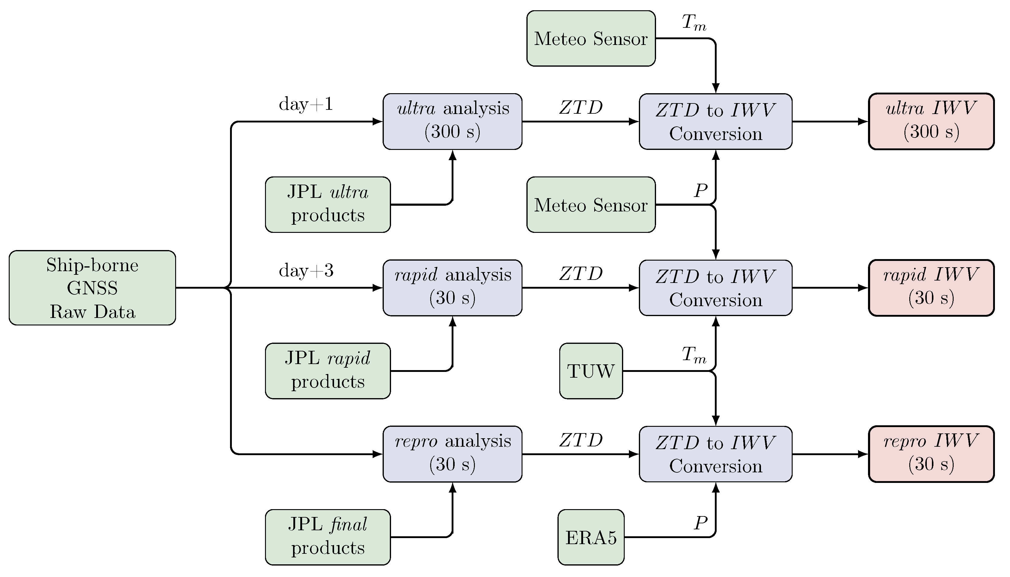
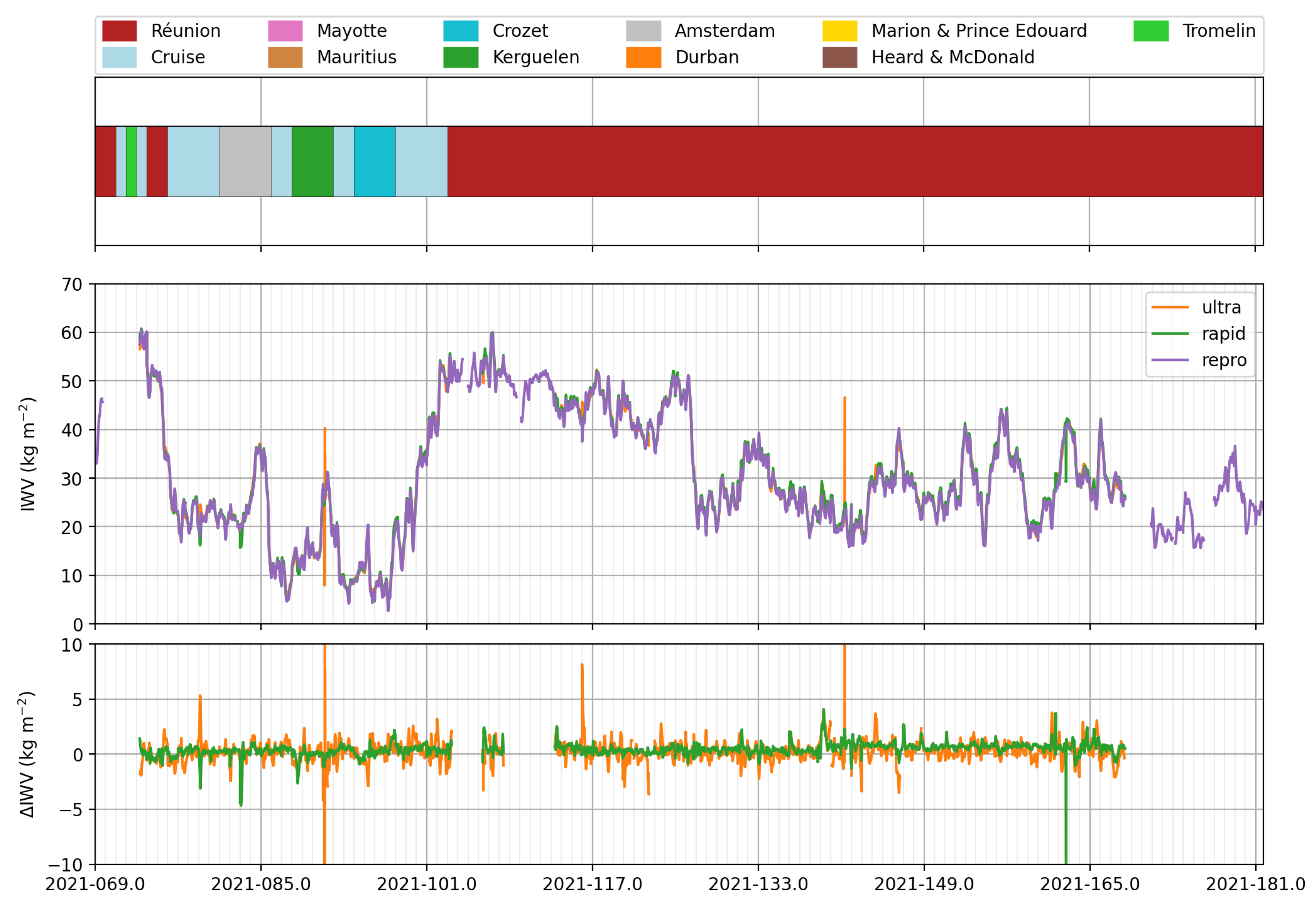
• Two operational daily routine analyses launched each day at day+1 (ultra) and day+3 (rapid). These analyses are intended to provide IWV retrieval with a low latency for short-term water vapour monitoring along the route of the vessel. These two routine analyses started from 14 March, after the change in location of the GNSS antenna on ship.
• One re-analysis of the raw data over the whole period (repro).

Note that GIPSY only allows post-processing of the acquired data with a minimum latency of about 1 h, which may limit its use for NWP issues. For real-time analysis of raw GNSS data, another processing tool should be preferred (e.g., RTKlib [39]).

The main characteristics of the three strategies are presented in

Table 1. GNSS analysis strategies; elevation cut-off angle, data weighting and ambiguity resolution are identical for the three analyses.

	ultra	rapid	repro
Elevation cut-off angle	3${}^{°}$
Data weighting	1 cm / $\sqrt{sin\left(elevation\right)}$
Ambiguity resolution	Yes
Orbits and clocks (sampling)	ultra-rapid (300 s)	rapid (30 s)	final (30 s)
Ionosphere model	Iono-free	Iono-free	Iono-free
			2nd order
Troposphere model	GPT	GPT	VMF1
	GMF	GMF	VMF1

. We used Jet Propulsion Laboratory (JPL) products for satellite orbits and clocks: ultra-rapid products, with a 300 s sampling, for the ultra analysis; rapid products, with a 30 s sampling, for the rapid analysis; final products, with a 30 s sampling, for the repro analysis. The phase and code raw data were analysed in a 30 h window centred on noon (GPS-Time) of each day from which the 00:00–24:00 parameters were extracted to avoid edge effects. Phase ambiguities were fixed using the wide-lane and phase bias information also provided by JPL [40]. The analysis is performed in a kinematic mode that estimates receiver position, clock offsets, zenith troposphere delays (ZTD) and troposphere horizontal gradients simultaneously for each epoch (sampling of 300 s for the ultra processing, 30 s for the two others). No constraint was applied to positions between consecutive epochs.

The troposphere effect on GNSS signal propagation was modelled by time-varying Zenith Hydrostatic Delays (ZHD), Zenith Wet Delays (ZWD) and horizontal gradients with a sampling of 30 s for rapid and repro and 300 s for ultra. A priori values for ZHDs and ZWDs were computed from ECMWF analysis (provided by TUV, https://vmf.geo.tuwien.ac.at/, accessed on 19 January 2022) for the repro processing; due to operational constraints, GPT model [41] is preferred for the ultra and rapid processing. Elevation dependency for both ZHD and ZWD is modelled by VMF1 mapping function [42] for the repro processing, and by GMF [43] mapping function for the rapid and ultra processing. The final GNSS ZTD are then obtained by the sum of ZHD and ZWD.

2.3. GNSS IWV Retrieval

The integrated water vapour content ($IWV$) is derived from the $ZTD$ estimates as:

$$IWV=\kappa \left(T_m\right)\times [ZTD-ZHD]$$

(1)

The $IWV$ is also related to the precipitable water vapour, $PWV$, by the relation [44]:

$$IWV={\rho }_w\times PWV$$

(2)

where ${\rho }_w$ is the liquid water density.

Here, $ZHD$ needs to be obtained from a more accurate method than the one used as a priori in the GNSS analysis (using, for example, surface pressure measurement or surface level pressure from a NWP reanalysis) [45]:

$$ZHD={10}^{-6}{k}_1{R}_d\frac{P}{g_m}$$

(3)

where $k_1=0.776452$ K Pa${}^{-1}$, is the dry air refractivity coefficient, $R_d=287.001$ J K kg${}^{-1}$ the dry air specific gas constant [22] and P the surface air pressure; $g_m$ is a parametric model for the mean acceleration due to gravity which depends on the latitude and ellipsoid height [46].

Since, the surface pressure value may be given for a slightly different height from the GNSS antenna, $ZHD$ may be extrapolated using the formulation proposed in [47] and already used in [23,32]:

$$ZHD\left(h\right)=ZHD(h+\mathsf{\Delta }h)-{10}^{-6}{k}_1\frac{P(h+\mathsf{\Delta }h)}{T(h+\mathsf{\Delta }h)}\times \frac{g(h+\mathsf{\Delta }h)}{g_{atm}}\times \mathsf{\Delta }h$$

(4)

where h is the ellipsoid height of the GNSS antenna, $\mathsf{\Delta }h$ is the difference in height between the GNSS antenna and the surface for pressure measurement; P is the pressure and T the temperature.

Finally, the conversion constant in Equation (1), $\kappa \left(T_m\right)$, is given by [14]:

$$\kappa \left(T_m\right)=\frac{{10}^6}{R_v(k_2^{\prime }+\frac{k_3}{T_m})}$$

(5)

where $R_v=461.522$ J ${\mathrm{K}}^{-1}$ kg${}^{-1}$ is the specific gas constant for water vapour, $k_2^{\prime }=k_2-k_1\frac{R_d}{R_v}=0.229$ K Pa${}^{-1}$, and $k_3=375.200$ K${}^2$ Pa${}^{-1}$ are refractivity coefficients for the water vapour [22]. $T_m$ is the weighted mean temperature [14].

From this, because of the latency in the availability of some data, different strategies are used for the ZTD to IWV conversion:

• ultra analysis: surface pressure measurements from a ship-borne meteorological sensor were used (Equation (3)) and extrapolated to GNSS antenna (Equation (4)); the weighted mean temperature was computed from $T_m=0.72\times T_d+70.2$ [14], where $T_d$ is the daily mean surface temperature [19], and used to compute $\kappa$ (Equation (5)).
• rapid analysis: surface pressure measurements from the ship-borne meteorological sensor were still used (Equation (3)) and extrapolated to GNSS antenna (Equation (4)); the weighted mean temperature was computed using global grid provided by TU Wien using a vertical extrapolation gradient of $-5.4$ K km${}^{-1}$ [17].
• repro analysis: the mean sea level pressure was extracted from ERA5 reanalysis with a horizontal resolution of 0.25${}^{°}$ and temporal sampling of 1 h [48]; the weighted mean temperature was computed using the global grid provided by TU Wien using a vertical extrapolation gradient of $-5.4$ K km${}^{-1}$ [17].

Figure 4 summarised the retrieval procedure from GNSS raw data to IWV.

Reference [49] presented a detailed error budget for ship-borne GNSS IWV retrieval and concluded with an uncertainty of shipborne GNSS IWV at 2.70 kg m${}^{-2}$. Although this value could be refined due to some differences in the ZTD estimation and the IWV conversion method (values and uncertainties for the constants of Equations (3)–(5); external data for surface pressure and mean temperature), we can reasonably expect an uncertainty of less than 3 kg m${}^{-2}$.

In order to identify and reject spurious estimates, a screening of the IWVs is performed from a range check on the formal errors for position and ZTD errors. The details of this screening are presented in

Table 2. Screening used for the GNSS estimates: threshold for range check on 3D position formal errors and ZTD formal errors; number of data points after screening and screening rejection rate. ${}^{*}$ corresponds to values that are computed after the change of the location of the antenna.

	${\mathit{R}\mathit{C}}_{{\mathit{\sigma }}_{\mathit{P}\mathit{O}\mathit{S}}}$ (mm)	${\mathit{R}\mathit{C}}_{{\mathit{\sigma }}_{\mathit{Z}\mathit{T}\mathit{D}}}$ (mm)	${\mathit{N}}_{\mathit{p}\mathit{t}\mathit{s}}$	${\%}_{\mathit{o}\mathit{u}\mathit{t}}$
ultra	0.1–1000	0.1–6.5	24,054	3.9
rapid	0.1–1000	0.1–3.0	249,734	0.2
repro	0.1–1000	0.1–3.0	729,868	1.9
repro${}^{*}$	0.1–1000	0.1–3.0	298,871	0.4

. The threshold values were established after a careful study of the formal error time series and distribution; the higher values used for the ultra solution are explained by the resolution of the calculation (300 s) which reduces the number of observations, decreases the redundancy, and thus induces an increase in the formal error. The rejection rate is the highest for the ultra analysis; it could be expected from the lowest accuracy of the ultra ephemerids and clocks and also by the lower time resolution of this analysis. For the repro processing, the screening rejection rate is considerably reduced after the change in location of the antenna on ship, from 1.9% to 0.4%, which corroborate the gain in quality due to this change. We also observe a larger number of rejected values for the repro solution than for the rapid solution: this difference is mainly due to the periods of interruption of the routine solutions around days 105, 109, 173 and 180 of 2021 (surface measurements data for IWV conversion were unavailable then) when a large number of outliers were rejected for the screening of the repro solution.

Figure 5 gives an overview of the final availability of GNSS IWV from the three analyses. Breaks include system failure of GNSS receiver, surface meteorological sensor interruption (affecting ultra and rapid retrieval), and outliers rejected by screening. For the ultra processing, 12.3% of the data is missing, with 14 interruptions longer than 30 min. For the rapid processing, 9.0% of the data is missing, with four interruptions longer than 30 min. Finally, For the repro processing, 7.4% of the expected data is missing, with 48 interruptions longer than 30 min.

3. Comparison Dataset

3.1. ERA5

The Total Column Water Vapour (TCWV) product form ERA5 reanalysis [48] is used to retrieve IWV estimates along the track. This product is provided with a horizontal sampling of 0.2$5^{°}$ and a time resolution of 1 h. Each 1-hour grid point surrounding the GNSS antenna was first extrapolated at the GNSS antenna height using the empirical gradient for IWV proposed by [50] and used in [17,23]:

$$IWV\left(h\right)=IWV(h+\mathsf{\Delta }h)\times \left[1-k\times \mathsf{\Delta }h\right]$$

(6)

where $k=4\times {10}^{-4}$ kg m${}^{-2}$ m${}^{-1}$.

The values are then bilinearly interpolating at the GNSS antenna horizontal position.

3.2. Ground-Launched Radiosonde

Two ground-launched radiosonde stations are considered: Le Gillot (Reunion Island) and Port-aux-Français (Kerguelen Island)—see Figure 1. For Le Gillot, two radiosondes are launched every day (at 11:15 and 23:15 UTC), while for Port-aux-Français only one day-time radiosonde is launched every day (at 11:15 UTC). Both stations used Modem M10 radiosondes and provide high vertical resolution profiles (about 5–10 m in the lower troposphere) of pressure, temperature and dew point temperature. A light quality check of the radiosondes profiles is performed: we only considered profiles that reach at least 10,000 m with a first point at most 5 m above the station (this check rejects 1.7% of the profiles for Le Gillot, 10% for Port-aux-Français); moreover, only ascending points are considered.

Various studies have already been conducted to evaluate the agreement of this type of radiosonde with other techniques or type of radiosondes. During a campaign dedicated to the evaluation of water vapour measurement methods, [16] presented large dry biases in humidity monitoring, especially in dry layers; this induced an overall dry bias in IWV retrieval compared to GNSS of about −12.6% and a standard deviation of 6.6%. More recently, [51] investigated the error sources that may degrade humidity measurements with Modem M10 radiosondes. They proposed a set of corrections that was shown to reduce differences with the well-known RS92 radiosonde by a factor of 2–3. However, this set of corrections is not yet implemented for all radiosonde stations. In another recent study, [19] presented differences in IWW retrieval from M10 and GNSS, with a bias of −1.93 kg m${}^{-2}$ (M10 dryer than GNSS).

Water vapour pressure of profiles are computed from dew-point temperature using Teten’s formula [52]. Then, IWV are obtained from the vertical interpolation of the water vapour density profiles from surface to the top of the profile:

$$IWV={\int }_{sfc}^{top}{\rho }_{wv}\left(h\right)dh$$

(7)

where ${\rho }_{wv}=\frac{e}{Rv\times T}$ is the water vapour density, e is Water vapour pressure, T is the temperature, $R_v$ = 461.522 J K${}^{-1}$ kg${}^{-1}$ is the specific gas constant for water vapour [22].

3.3. Ground GNSS Antenna

Along its track, the R/V Marion Dufresne passed close to ground continuously operating reference GNSS stations (CORS) as indicated in Figure 1. For each territory highlighted on the map, only one reference station was considered, the selection criteria being based on data availability, proximity of the station to the coastline and to mean sea level.

The GNSS raw data was also analysed using GIPSY, following a procedure that has been widely used in previous studies [22,23]. Hereafter, we present the main characteristics of the processing. Only GNSS data for the GPS constellation is considered and processed in PPP mode with ambiguity resolution; we used JPL final products for orbits and clocks of GPS satellites. Analysis was performed in static mode with the estimation of one single position per day for each station. ZWDs and horizontal gradients were estimated after a priori correction for ZHD and ZWD from ECMWF analysis, with a sampling of 300 s. Elevation dependency for troposphere delays was modelled by VMF1 mapping function. As for the ship-borne ZTDs, a screening of the ground estimated ZTDs was also performed in order to reject spurious data or outliers that would degrade comparisons. The screening was reduced to a range check on the formal errors of the estimated ZTDs. The threshold value of 4.0 mm was chosen on the basis of the distribution of formal errors over the period of interest. This threshold induces a low rejection rate in the range 0.0–0.1% except for the station DRBA, where it reaches 17.8%. This large rate may be linked to a large number of interruptions of acquisition from this antenna over the period.

Finally, IWV of CORS are retrieved for ZTD estimates using the same methodology as for the ship-borne repro solution.

4. Assessment of GNSS IWV Retrieval

An assessment of GNSS-derived IWV was conducted using estimates from the repro processing, from Oct. 2020 to Jun. 2021. We used IWV from the seven ground reference GNSS antennas, the two radiosonde sites (see Figure 1) and the ERA5 reanalysis for comparisons.

The Figure 6 shows the IWV times series from the different techniques. Overall, there is good consistency between the different sources of IWV. However, we should note the radiosondes, which occasionally deviate more strongly from the other techniques (in particular for the radiosondes launched at Réunion Island). It is easy to distinguish the different climatic zones crossed, with the drier southern passages (between Crozet, Kerguelen, Marion and Prince Edouard islands), with IWVs fluctuating around 15 kg m${}^{-2}$ and extreme values between 5 and 30 kg m${}^{-2}$, and the passages closer to the tropics (Réunion Mayotte, Mauritus), more humid, where IWVs fluctuate around 30 kg m${}^{-2}$ for extreme values between 20 and 65 kg m${}^{-2}$, which may be usual in tropical areas [29,53]. The long docking period in Réunion Island in spring 2021 is due to health constraints related to the COVID-19 pandemic.

Furthermore, it is worth noting:

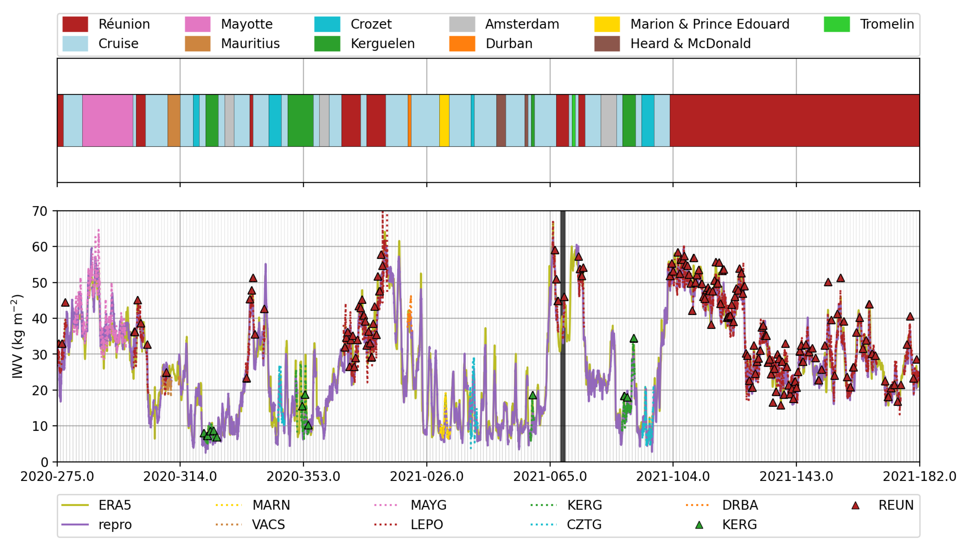
• The passage in the southern part of the Indian Ocean in February 2021 (days 30 to 60), with a succession of dry (<10 kg m${}^{-2}$) and wet (IWV $>30$ kg m${}^{-2}$) periods.
• A very wet period in early January 2021 near Reunion (days 11–13 of 2021, peak IWV above 60 kg m${}^{-2}$), coinciding with the passage of tropical storm Danilo.
• A very wet period in early March 2021 between Reunion and Tromelin (around day 65 of 2021, IWV $>60$ kg m${}^{-2}$), corresponding with the passage of tropical storm Iman.
• A long wet period when the Marion Dufresne was docked in Reunion during the last two weeks of April (around days 104 to 125, IWV around 50 kg m${}^{-2}$), corresponding to a very rainy sequence on the island, with a cumulative rainfall twice as high as the seasonal normal.

Differences of IWV retrieval from ERA5, CORS and radiosondes with respect to the ship-borne IWV (repro analysis) are computed by time matching and summarised in

Table 3. Statistics of difference with respect to the repro solution: comparisons with IWV retrievals from ERA5, CORS and radiosoundings. $N_{pts}$: number of data points; $\mu$ mean IWV (kg m${}^{-2}$); $b\pm \sigma$: bias ± standard-deviation of differences (kg m${}^{-2}$); rms: difference root mean square (kg m${}^{-2}$); $\rho$: correlation coefficient; d: mean distance between CORS or radiosonde station and the R/V (km); $\mathsf{\Delta }h$: mean difference in height between CORS or radiosonde station and the R/V (m). Lines marked with a ${}^{*}$ show the statistics after changing the position of the antenna on the ship.

	${\mathit{N}}_{\mathit{p}\mathit{t}\mathit{s}}$	$\mathit{\mu }$	$\mathit{b}\pm \mathit{\sigma }$	rms	$\mathit{\rho }$	d	$\mathbf{\Delta }\mathit{h}$
ERA5	6055	26.6	+0.21 ± 2.78	2.79	+0.98	-	-
ERA5 ${}^{*}$	2490	30.4	+0.45 ± 2.45	2.49	+0.98	-	-
CORS
CZTG	1800	+12.6	−0.08 ± 2.69	2.70	+0.90	9.5	120
KERG	3168	+12.0	+1.13 ± 2.47	2.71	+0.92	6.6	3
MARN	453	+10.7	+2.64 ± 2.50	3.63	+0.80	27.9	−12
LEPO	26,750	+34.5	+0.47 ± 2.15	2.21	+0.98	3.7	−13
MAYG	3922	+41.2	+0.35 ± 3.49	3.51	+0.88	23.1	−21
DRBA	65	+39.3	+0.66 ± 1.12	1.30	−0.43	21.3	7
VACS	573	+23.1	−2.30 ± 2.10	3.11	+0.29	26.3	398
CZTG ${}^{*}$	933	+9.2	−0.00 ± 2.84	2.84	+0.71	4.5	115
KERG ${}^{*}$	1055	+17.4	+0.31 ± 1.56	1.59	+0.97	5.0	−2
LEPO ${}^{*}$	20,485	+34.0	+0.60 ± 1.74	1.84	+0.99	3.3	−15
Radiosondes
REUN	153	+36.9	+2.54 ± 3.45	4.29	+0.96	26.3	11
KERG	11	+13.9	+2.36 ± 2.70	3.59	+0.94	5.0	0
REUN ${}^{*}$	116	+36.1	+2.28 ± 3.30	4.01	+0.97	25.9	9

. For CORS and radiosondes comparisons, we only considered data points when antennas were closer than 50 km.

The bias between the ERA5 and repro is quite small (0.21 kg m${}^{-2}$), with ERA5 being wetter than GNSS. This bias tends to increase after the change of the location of the antenna (0.45 kg m${}^{-2}$). One explanation for this increase may lie in the fact that the Marion Dufresne was docked in Reunion for a long time after the antenna change; at this location, one of the surrounding ERA5 grid points is on the western slope of the Python des Neiges: extrapolating the ERA5 value at this point to the height of the GNSS antenna may degrade the quality the extracted IWV value. The difference rms is also clearly reduced after changing the location of the antenna (from 2.79 to 2.49 kg m${}^{-2}$). The values (before and after the change of location of the antenna) are fairly consistent with the values already cited in the literature [32,49]; [33] provide lower rms difference between GNSS and ERA5 for an experiment performed in the Arctic Ocean, but it is known that in such areas, the low space and time distribution of water vapour may be more easy for the ERA5 to catch.

Regarding the comparison with CORS during the whole period, we observe a difference in rms of between 1.30 and 3.63 kg m${}^{-2}$, with biases that range from $-2.30$ to $2.64$ kg m${}^{-2}$. Mean IWV values range from 10.7 to 41.2 kg m${}^{-2}$ and are higher for low latitude stations (MAYG, LEPO) than for high latitude stations (CZTG, KERG, MARN). This was obviously expected, as a warm atmosphere can contain more water vapour than a cold atmosphere. Two stations present larger biases: for the station VACS, this large value can be attributed to the large difference in altitude between the two antennas (nearly 400 m); the large bias for station MARN is not yet explained, but might be linked to the small period of comparison and the largest distance between ship-borne and ground GNSS antenna (27.9 km in average), and/or the unfavourable location of the GNSS antenna on the ship at this time. Despite a good agreement in terms of differences (0.66 ± 1.12 kg m${}^{-2}$), comparison with DRBA station highlights a poor correlation coefficient (0.29); this can be linked to a low number of comparison points. Stations KERG and CZTG present similar differences, with a lower bias for CZTG (−0.08 kg m${}^{-2}$) and a smaller standard-deviation for KERG (2.47 kg m${}^{-2}$), with similar mean IWV values (around 12 kg m${}^{-2}$). Station MAYG, which is the closest CORS to the equator, presents the highest mean IWV value (41.2 kg m${}^{-2}$) and the highest difference rms too (3.51 kg m${}^{-2}$); such order of magnitude of differences with CORS were also observed over the Tropics in [32,49]. Station LEPO provide the largest number of comparison points, with a good agreement (rms of 2.21 kg m${}^{-2}$ for the whole period); It should be noted, however, that these good results were obtained under quite favourable conditions, as the proximity to the LEPO station corresponds to a dockside position of the R/V. Finally, we observe a clear improvement in the comparisons with KERG and LEPO when considering the period after the change in location of the antenna on the ship (difference rms decrease respectively from 2.71 to 1.59 kg m${}^{-2}$ and 2.21 to 1.84 kg m${}^{-2}$). For CZTG, the bias is reduced but the standard deviation slightly increases.

Comparisons with radiosondes exhibit a large difference in rms (4.29 kg m${}^{-2}$ and 3.59 kg m${}^{-2}$ for REUN and KERG, respectively) and bias (2.54 kg m${}^{-2}$ and 2.36 kg m${}^{-2}$ for REUN and KERG, respectively), with radiosonde wetter than ship-borne GNSS. These differences are larger than those presented in the majority of previous studies [33,49], even if larger ones are also observed [54]. We have previously mentioned that such radiosondes (Modem M10) were mainly known to have dry bias, which is not the case here. We also compared radiosonde IWV to IWV from closest CORS station (LEPO and KERG) over the whole period (435 profiles for REUN, 237 for KERG); wet biases (radiosonde wetter than CORS) were also observed (1.13 kg m${}^{-2}$ for KERG, 2.65 kg m${}^{-2}$ for REUN). Radiosondes profiles were also investigated. Relative humidity saturation in the lower layers was commonly observed (range 0–3 km for REUN, 0-1 km for KERG, not shown here) and may explain the highest IWV values. Currently, the cause of this saturation was not elucidated; some hypothesis has been put forward, such as radiosonde assent through deep clouds and precipitation or water vapour condensation on the its humidity sensor.

5. Operational Production of GNSS Derived IWV

Figure 7 shows the time series of the integrated water vapour contents of the three solutions presented previously (ultra, rapid and repro) as well as the deviations of the operational analysis from the repro analysis. During this period of comparison, the Marion Dufresne is, for the most part, docked in Reunion Island; this may tend to improve the results of the analyses and therefore overestimate the performance of the operational calculations. As mentioned previously, breaks in ultra and rapid solution are mainly due to interruptions in surface meteorological sensor (that is use for ZTD to IWV conversion). There is a good overall consistency between the three solutions; the time series for the ultra analysis show abrupt variations inherent to the lower accuracy and resolution of the ephemeris used. Whether the vessel is docked, anchored or on the open sea, the differences between the repro solution and the rapid solution are in the ±5 kg m${}^{-2}$ range (except one outlying point on day 162 that was not rejected by the screening). Over the period, the differences between the ultra and repro solutions are greater than 2 kg m${}^{-2}$ for only 0.3% of the points compared. Between the rapid and repro analyses, this rate is slightly higher, around 1.3%.

The statistics of the differences to the repro solution are presented in the

Table 4. Statistics of difference with respect to the repro solution of the two operational solutions, ultra and rapid. $N_{pts}$—number of data points; $\mu$—mean IWV (kg m${}^{-2}$); $b\pm \sigma$—bias ± standard deviation of differences (kg m${}^{-2}$); rms—root mean square of differences (kg m${}^{-2}$); $\rho$—correlation coefficient.

	${\mathit{N}}_{\mathit{p}\mathit{t}\mathit{s}}$	$\mathit{\mu }$	$\mathit{b}\pm \mathit{\sigma }$	rms	$\mathit{\rho }$
ultra	24,022	+29.3	+0.24 ± 1.00	1.03	+1.00
rapid	249,481	+29.5	+0.43 ± 0.59	0.73	+1.00

. The biases are small (less than 0.5 kg m${}^{-2}$); for the ultra solution, they are linked to the differences in the estimated ZTDs, to the differences in ZHDs (PTU vs. ERA5) and to the difference in $T_m$ (PTU vs. VMF1). For the rapid solution, the bias is only due to the differences in estimated ZTD and calculated ZHD. The standard deviations of the differences are reduced with the rapid analysis compared to the ultra analysis (1.00 kg m${}^{-2}$ for the ultra analysis down to 0.59 kg m${}^{-2}$ for the rapid analysis). The correlation coefficients of 1.00 highlight the high consistency of the time series. These statistics highlight the performance of the routine IWV retrieval with a low latency (from 1 to 3 days).

6. Discussion and Conclusions

In this study, we presented the IWV retrieval from a ship-borne GNSS antenna on the R/V Marion Dufresne as part of the MAP-IO project. The antenna was installed in October 2020 and has been operating continuously since then. The IWV retrieval aims at the long-term documentation, description and understanding of the space and time distribution of atmospheric water vapour over the Indian and Austral Oceans.

GNSS raw data are uploaded daily on an FTP server. A preliminary study of the raw data revealed an unfavourable location of the antenna on the ship. The change of its location was shown to reduce both multipath and cycle slips, which can severely degrade the results of GNSS analysis. In March 2021, two daily routine processing streams of the GNSS raw data were set up, with a latency of 1 and 3 days, respectively. They are intended to provide accurate and operational GNSS-based IWV to the scientific community. In parallel, a “reprocessing” analysis was carried out in order to obtain a long series of IWV since the installation of the antenna.

The reprocessing analysis was compared to IWVs extracted from ERA5, or measured by GNSS CORS and ground-launched radiosondes. The differences between the techniques are consistent with results from previous studies, with difference rms of 2.79 kg m${}^{-2}$ for ERA5, 1.30 to 3.6 kg m${}^{-2}$ for CORS and 3.59 to 4.29 kg m${}^{-2}$ for radiosondes. Differences were shown to be reduced after the change in location of the antenna on the ship. These results confirm the good performance of IWV restitution from a shipboard antenna. Next, the routine analyses were compared with the reprocessing analysis. A very good match is observed with the reprocessing analysis showing low difference rms and high correlation coefficient. These results highlight the performance of a routine observation of water vapour over the oceans with the help of ship-borne GNSS antennas.

The deployment of the GNSS antenna on the R/V Marion Dufresne is now sustainable. The IWV measurements retrieved, as presented in this study, will be used for long-term periods, as it is customary for ground-based antennas. Rms difference of routine analysis are consistent with threshold requirement mentioned by [55] for global and regional NWP, but the latency should be still reduced. This could be reached thanks to the maritime VSAT carried on the R/V Marion Dufresne. An hourly transmission of GNSS raw data is thus expected in the near future and will enable an hourly analysis with a latency of a few hours (typically below 2 h). The operational use of ship-borne GNSS IWV as assimilated data in NWP thus becomes reachable.

Further assessments of GNSS and IWV data quality collected onboard the RV Marion Dufresne will be conducted in the near future through organising dedicated GNSS verification experiments, based on the launch of collocated radiosondes onboard the vessel and also on the use of satellite-borne water vapour measurements [49,56]. Moreover, further intercomparison procedures will also be set up in the the tropical Indian Ocean to benefit from the recent, and relatively dense, ground-based GNSS network deployed in Madagascar and Scattered Island of Grande Glorieuse, Juan de Nova, Europa and Tromelin in the frame of the IOGA4MET research program [57,58].

References

1. Bengtsson, L. The global atmospheric water cycle. Environ. Res. Lett. 2010, 5, 025202. [Google Scholar] [CrossRef]
2. Dessler, A.E.; Zhang, Z.; Yang, P. Water-vapor climate feedback inferred from climate fluctuations, 2003–2008. Geophys. Res. Lett. 2008, 35, L20704. [Google Scholar] [CrossRef] [Green Version]
3. Corringham, T.W.; Martin Ralph, F.; Gershunov, A.; Cayan, D.R.; Talbot, C.A. Atmospheric rivers drive flood damages in the western United States. Sci. Adv. 2019, 5, eaax4631. [Google Scholar] [CrossRef] [Green Version]
4. Binder, H.; Riviere, G.; Abrogast, P.; Maynard, K.; Bosser, P.; Joly, B.; Labadie, C. Dynamics of forecast error growth along cut-off Sanchez and its consequence for the prediction of a high-impact weather event over southern France. Q. J. R. Meteorol. Soc. 2021, 147, 3263–3285. [Google Scholar] [CrossRef]
5. Ducrocq, V.; Braud, I.; Davolio, S.; Ferretti, R.; Flamant, C.; Jansa, A.; Kalthoff, N.; Richard, E.; Taupier-Letage, I.; Ayral, P.A.; et al. HyMeX-SOP1: The Field Campaign Dedicated to Heavy Precipitation and Flash Flooding in the Northwestern Mediterranean. Bull. Am. Meteorol. Soc. 2014, 95, 1083–1110. [Google Scholar] [CrossRef]
6. Trenberth, K.E.; Smith, L.; Qian, T.; Dai, A.; Fasullo, J. Estimates of the Global Water Budget and Its Annual Cycle Using Observational and Model Data. J. Hydrometeorol. 2007, 8, 758–769. [Google Scholar] [CrossRef]
7. Nuissier, O.; Ducrocq, V.; Ricard, D.; Lebeaupin, C.; Anquetin, S. A numerical study of three catastrophic precipitating events over southern France. I: Numerical framework and synoptic ingredients. Q. J. R. Meteorol. Soc. 2008, 134, 111–130. [Google Scholar] [CrossRef]
8. Kato, T. Quasi-stationary Band-Shaped Precipitation Systems, Named “Senjo-Kousuitai”, Causing Localized Heavy Rainfall in Japan. J. Meteorol. Soc. Japan. Ser. II 2020, 98, 485–509. [Google Scholar] [CrossRef] [Green Version]
9. Smith, S.R.; Alory, G.; Andersson, A.; Asher, W.; Baker, A.; Berry, D.I.; Drushka, K.; Figurskey, D.; Freeman, E.; Holthus, P.; et al. Ship-Based Contributions to Global Ocean, Weather, and Climate Observing Systems. Front. Mar. Sci. 2019, 6, 434. [Google Scholar] [CrossRef] [Green Version]
10. Gao, B.C.; Kaufman, Y.J. Water vapor retrievals using Moderate Resolution Imaging Spectroradiometer (MODIS) near-infrared channels. J. Geophys. Res. 2003, 108. [Google Scholar] [CrossRef]
11. Mears, C.A.; Smith, D.K.; Ricciardulli, L.; Wang, J.; Huelsing, H.; Wentz, F.J. Construction and Uncertainty Estimation of a Satellite-Derived Total Precipitable Water Data Record Over the World’s Oceans. Earth Space Sci. 2018, 5, 197–210. [Google Scholar] [CrossRef] [Green Version]
12. Yoneyama, K.; Zhang, C.; Long, C.N. Tracking Pulses of the Madden–Julian Oscillation. Bull. Am. Meteorol. Soc. 2013, 94, 1871–1891. [Google Scholar] [CrossRef]
13. Guerova, G.; Jones, J.; Douša, J.; Dick, G.; de Haan, S.; Pottiaux, E.; Bock, O.; Pacione, R.; Elgered, G.; Vedel, H.; et al. Review of the state of the art and future prospects of the ground-based GNSS meteorology in Europe. Atmos. Meas. Tech. 2016, 9, 5385–5406. [Google Scholar] [CrossRef] [Green Version]
14. Bevis, M.; Bussinger, S.; Herring, T.A.; Rocken, C.; Anthes, R.A.; Ware, R.H. GPS Meteorology: Remote Sensing of Atmospheric Water Vapor Using the Global Positioning System. J. Geophys. Res. 1992, 97, 15787–15801. [Google Scholar] [CrossRef]
15. Haase, J.; Ge, M.; Vedel, H.; Calais, E. Accuracy and Variability of GPS Tropospheric Delay Measurements of Water Vapor in the Western Mediterranean. J. Appl. Meteorol. 2003, 42, 1547–1568. [Google Scholar] [CrossRef]
16. Bock, O.; Bosser, P.; Bourcy, T.; David, L.; Goutail, F.; Hoareau, C.; Keckhut, P.; Legain, D.; Pazmino, A.; Pelon, J.; et al. Accuracy assessment of water vapour measurements from in situ and remote sensing techniques during the DEMEVAP 2011 campaign at OHP. Atmos. Meas. Tech. 2013, 6, 2777–2802. [Google Scholar] [CrossRef] [Green Version]
17. Parracho, A.C.; Bock, O.; Bastin, S. Global IWV trends and variability in atmospheric reanalyses and GPS observations. Atmos. Chem. Phys. 2018, 18, 16213–16237. [Google Scholar] [CrossRef] [Green Version]
18. Bock, O.; Parracho, A.C. Consistency and representativeness of integrated water vapour from ground-based GPS observations and ERA-Interim reanalysis. Atmos. Chem. Phys. 2019, 19, 9453–9468. [Google Scholar] [CrossRef] [Green Version]
19. Lees, E.; Bousquet, O.; Leclair De Bellevue, J. Analysis of diurnal to seasonal variability of Integrated Water Vapour in the South Indian Ocean basin using ground-based GNSS and fifth-generation ECMWF reanalysis (ERA5) data. Q. J. R. Meteorol. Soc. 2020, 1–20. [Google Scholar] [CrossRef]
20. Van Baelen, J.; Reverdy, M.; Tridon, F.; Labbouz, L.; Dick, G.; Bender, M.; Hagen, M. On the relationship between water vapour field evolution and the life cycle of precipitation systems. Q. J. R. Meteorol. Soc. 2011, 137, 204–223. [Google Scholar] [CrossRef] [Green Version]
21. Bock, O.; Bosser, P.; Pacione, R.; Nuret, M.; Fourrié, N.; Parracho, A. A high-quality reprocessed ground-based GPS dataset for atmospheric process studies, radiosonde and model evaluation, and reanalysis of HyMeX Special Observing Period. Q. J. R. Meteorol. Soc. 2016, 142, 56–71. [Google Scholar] [CrossRef]
22. Bock, O.; Bosser, P.; Flamant, C.; Doerflinger, E.; Jansen, F.; Fages, R.; Bony, S.; Schnitt, S. IWV observations in the Caribbean Arc from a network of ground-based GNSS receivers during EUREC4A. Earth Syst. Sci. Data 2021. [Google Scholar] [CrossRef]
23. Bosser, P.; Bock, O. IWV retrieval from ground GNSS receivers during NAWDEX. Adv. Geosci. 2021, 55, 13–22. [Google Scholar] [CrossRef]
24. Poli, P.; Moll, P.; Rabier, F.; Desroziers, G.; Chapnik, B.; Berre, L.; Healy, S.B.; Andersson, E.; El Guelai, F.Z. Forecast impact studies of zenith total delay data from European near real-time GPS stations in Météo-France 4DVAR. J. Geophys. Res. 2007, 112, D06114. [Google Scholar] [CrossRef]
25. Bennitt, G.V.; Jupp, A. Operational Assimilation of GPS Zenith Total Delay Observations intothe Met Office Numerical Weather Prediction Models. Mon. Weather Rev. 2012, 140, 2706–2719. [Google Scholar] [CrossRef]
26. Mahfouf, J.F.; Ahmed, F.; Moll, P.; Teferle, F.N. Assimilation of zenith total delays in the AROME France convective scale model: A recent assessment. Tellus A Dyn. Meteorol. Oceanogr. 2015, 67, 26106. [Google Scholar] [CrossRef]
27. Chadwell, C.D.; Bock, Y. Direct estimation of absolute precipitable water in oceanic regions by GPS tracking of a coastal buoy. Geophys. Res. Lett. 2001, 28, 3701–3704. [Google Scholar] [CrossRef]
28. Fujita, M.; Kimura, F.; Yoneyama, K.; Yoshizaki, M. Verification of precipitable water vapor etimated from shipborne GPS measurements. Geophys. Res. Lett. 2008, 35, L13803. [Google Scholar] [CrossRef]
29. Adams, D.K.; Fernandes, R.M.S.; Maia, J.M.F. GNSS Precipitable Water Vapor from an Amazonian Rain Forest Flux Tower. J. Atmos. Ocean. Technol. 2011, 28, 1192–1198. [Google Scholar] [CrossRef]
30. Boniface, K.; Champollion, C.; Chery, J.; Ducrocq, V.; Rocken, C.; Doerflinger, E.; Collard, P. Potential of shipborne GPS atmospheric delay data for prediction of Mediterranean intense weather events. Atmos. Sci. Lett. 2012, 13, 250–256. [Google Scholar] [CrossRef]
31. Wang, J.; Wu, Z.; Semmling, M.; Zus, F.; Gerland, S.; Ramatschi, M.; Ge, M.; Wickert, J.; Schuh, H. Retrieving Precipitable Water Vapor From Shipborne Multi-GNSS Observations. Geophys. Res. Lett. 2019, 46, 5000–5008. [Google Scholar] [CrossRef] [Green Version]
32. Bosser, P.; Bock, O.; Flamant, C.; Bony, S.; Speich, S. Integrated water vapour content retrievals from ship-borne GNSS receivers during EUREC4A. Earth Syst. Sci. Data 2021, 13, 1499–1517. [Google Scholar] [CrossRef]
33. Männel, B.; Zus, F.; Dick, G.; Glaser, S.; Semmling, M.; Balidakis, K.; Wickert, J.; Maturilli, M.; Dahlke, S.; Schuh, H. GNSS-based water vapor estimation and validation during the MOSAiC expedition. Atmos. Meas. Tech. 2021, 14, 5127–5138. [Google Scholar] [CrossRef]
34. Liu, Y.; Liu, Y.; Chen, G.; Wu, Z. Evaluation of HY-2A satellite-borne water vapor radiometer with shipborne GPS and GLONASS observations over the Indian Ocean. GPS Solut. 2019, 23, 23–87. [Google Scholar] [CrossRef]
35. Wu, Z.; Liu, Y.; Liu, Y.; Wang, J.; He, X.; Xu, W.; Ge, M.; Schuh, H. Validating HY-2A CMR precipitable water vapor using ground-based and shipborne GNSS observations. Atmos. Meas. Tech. 2020, 13, 4963–4972. [Google Scholar] [CrossRef]
36. Ikuta, Y.; Seko, H.; Shoji, Y. Assimilation of shipborne precipitable water vapour by Global Navigation Satellite Systems for extreme precipitation events. Q. J. R. Meteorol. Soc. 2021, 148, 57–75. [Google Scholar] [CrossRef]
37. Zumberge, J.F.; Heflin, M.B.; Jefferson, D.C.; Watkins, M.M. Precise point positioning for the efficient and robust analysis of GPS data from large networks. J. Geophys. Res. 1997, 102, 5005–5017. [Google Scholar] [CrossRef] [Green Version]
38. Estey, L.; Meertens, C. TEQC: The Multi-Purpose Toolkit for GPS/GLONASS Data. GPS Solut. 1999, 3, 42–49. [Google Scholar] [CrossRef]
39. Shoji, Y.; Sato, K.; Yabuki, M.; Tsuda, T. Comparison of shipborne GNSS-derived precipitable water vapor with radiosonde in the western North Pacific and in the seas adjacent to Japan. Earth Planets Space 2017, 69, 153. [Google Scholar] [CrossRef]
40. Bertiger, W.; Desai, S.D.; Haines, B.; Harvey, N.; Moore, A.W.; Owen, S.; Weiss, J.P. Single receiver phase ambiguity resolution with GPS data. J. Geod. 2010, 84, 327–337. [Google Scholar] [CrossRef]
41. Boehm, J.; Heinkelmann, R.; Schuh, H. Short Note: A global model of pressure and temperature for geodetic applications. J. Geod. 2007, 81, 679–683. [Google Scholar] [CrossRef]
42. Boehm, J.; Werl, B.; Schuh, H. Troposphere mapping functions for GPS and very long baseline interferometry from European Centre for Medium-Range Weather Forecasts operational analysis data. J. Geophys. Res. 2006, 11, B02406. [Google Scholar] [CrossRef]
43. Boehm, J.; Niell, A.E.; Tregoning, P.; Schuh, H. The Global Mapping Function (GMF): A new empirical mapping function based on numerical weather model data. Geophys. Res. Lett. 2006, 33, L07304. [Google Scholar] [CrossRef] [Green Version]
44. Adams, D.K.; Gutman, S.I.; Holub, K.L.; Pereira, D.S. GNSS observations of deep convective time scales in the Amazon. Geophys. Res. Lett. 2013, 40, 2818–2823. [Google Scholar] [CrossRef]
45. Davis, J.L.; Herring, T.A.; Shapiro, I.I.; Rogers, A.E.E.; Elgered, G. Geodesy by radio interferometry: Effects of atmospheric modeling errors on estimates of baseline length. Radio Sci. 1985, 20, 1593–1607. [Google Scholar] [CrossRef]
46. Bosser, P.; Bock, O.; Pelon, J.; Thom, C. An improved mean gravity model for GPS hydrostatic delay calibration. Geosci. Remote Sens. Lett. 2007, 4, 3–7. [Google Scholar] [CrossRef]
47. Steigenberger, P.; Boehm, J.; Tesmer, V. Comparison of GMF/GPT with VMF1/ECMWF and implications for atmospheric loading. J. Geod. 2009, 83, 943–951. [Google Scholar] [CrossRef]
48. Hersbach, H.; Bell, B.; Berrisford, P.; Hirahara, S.; Horányi, A.; Muñoz-Sabater, J.; Nicolas, J.; Peubey, C.; Radu, R.; Schepers, D.; et al. The ERA5 global reanalysis. Q. J. R. Meteorol. Soc. 2020, 146, 1999–2049. [Google Scholar] [CrossRef]
49. Wu, Z.; Lu, C.; Zheng, Y.; Liu, Y.; Liu, Y.; Xu, W.; Jin, K.; Tang, Q. Evaluation of Shipborne GNSS Precipitable Water Vapor Over Global Oceans From 2014 to 2018. IEEE Trans. Geosci. Remote Sens. 2022, 60, 1–15. [Google Scholar] [CrossRef]
50. Bock, O.; Keil, C.; Richard, E.; Flamant, C.; Bouin, M.N. Validation of precipitable water from ECMWF model analyses with GPS and radiosonde data during the MAP SOP. Q. J. R. Meteorol. Soc. 2005, 131, 3013–3036. [Google Scholar] [CrossRef]
51. Dupont, J.C.; Haeffelin, M.; Badosa, J.; Clain, G.; Raux, C.; Vignelles, D. Characterization and Corrections of Relative Humidity Measurement from Meteomodem M10 Radiosondes at Midlatitude Stations. J. Atmos. Ocean. Technol. 2020, 37, 857–871. [Google Scholar] [CrossRef] [Green Version]
52. Tetens, O. Über einige meteorologische Begriff. Zeitschrift für Geophys. 1930, 6, 297–309. [Google Scholar]
53. Bock, O.; Bouin, M.N.; Doerflinger, E.; Collard, P.; Masson, F.; Meynadier, R.; Nahmani, S.; Koité, M.; Gaptia Lawan Balawan, K.; Didé, F.; et al. West African Monsoon observed with ground-based GPS receivers during African Monsoon Multidisciplinary Analysis (AMMA). J. Geophys. Res. 2008, 113, 21005. [Google Scholar] [CrossRef] [Green Version]
54. Sohn, D.Y.; Choi, B.K.; Park, Y.; Kim, Y.C.; Ku, B. Precipitable Water Vapor Retrieval from Shipborne GNSS Observations on the Korean Research Vessel ISABU. Sensors 2020, 20, 4261. [Google Scholar] [CrossRef] [PubMed]
55. Offiler, D. EIG EUMETNET GNSS Vater Vapour Program: Products Requirements Document Version 1.0.; Technical Report; EUMETNET: Brussels, Belgium, 2010. [Google Scholar]
56. Gong, Y.; Liu, Z.; Foster, J.H. Evaluating the Accuracy of Satellite-Based Microwave Radiometer PWV Products Using Shipborne GNSS Observations Across the Pacific Ocean. IEEE Trans. Geosci. Remote Sens. 2022, 60, 1–10. [Google Scholar] [CrossRef]
57. Bousquet, O.; Lees, E.; Durand, J.; Peltier, A.; Duret, A.; Mekies, D.; Boissier, P.; Donal, T.; Fleischer-Dogley, F.; Zakariasy, L. Densification of the Ground-Based GNSS Observation Network in the Southwest Indian Ocean: Current Status, Perspectives, and Examples of Applications in Meteorology and Geodesy. Front. Earth Sci. 2020, 8, 566105. [Google Scholar] [CrossRef]
58. Bousquet, O.; Barruol, G.; Cordier, E.; Barthe, C.; Bielli, S.; Calmer, R.; Rindraharisaona, E.; Roberts, G.; Tulet, P.; Amelie, V.; et al. Impact of Tropical Cyclones on Inhabited Areas of the SWIO Basin at Present and Future Horizons. Part 1: Overview and Observing Component of the Research Project RENOVRISK-CYCLONE. Atmosphere 2021, 12, 544. [Google Scholar] [CrossRef]
Figure 1. R/V Marion Dufresne tracks from 1 October 2020 to 30 June 2021 (black line); blue circles denote ground GNSS reference stations; orange triangles denote ground-based radiosounding stations; coloured bold lines correspond to the different geographical zones that are crossed during the period.
Atmosphere 13 00903 g001
Figure 2. Daily quality check diagnostics of GPS phase observations for the period of interest: on the upper panel, MP1 (red) and MP2 (blue) are multipath combinations for L1 and L2 carrier; on the lower panel, O/S is the ratio between complete observations and the number of slips.
Atmosphere 13 00903 g002
Figure 3. Schematic view of the R/V Marion Dufresne. The coloured circles denote the successive location of the GNSS antenna on ship: in red, the first location (from 1 October 2020 to 10 March 2021); in green the second location (from 10 March 2021). Schematic view is courtesy of Nicolas Marquestaut (OSU-R/LACy).
Atmosphere 13 00903 g003
Figure 4. Workflow of IWV retrieval procedure from ship-borne GNSS raw data.
Atmosphere 13 00903 g004
Figure 5. Final availability of the GNSS derived IWV from the three GNSS data streams. The thick vertical black line denotes the change of antenna location on ship. Vertical red marks denote interruptions in IWV retrieval due to interruptions in GNSS raw data or meteorological measurements acquisition.
Atmosphere 13 00903 g005
Figure 6. IWV time series along the route of the R/V Marion Dufresne. The upper panel of the figure indicates the location of the R/V Marion Dufresne. The lower panels represent the IWV time series as seen by the Marion Dufresne (purple solid line, repro solution), ERA5 (olive solid line), CORS (dotted lines; MARN, VACS, MAYG, LEPO, KERG, CZTG and DRBA) and radiosondes (triangles, REUN and KERG); the thick vertical black line denotes the change of antenna location on the ship.
Atmosphere 13 00903 g006
Figure 7. IWV time series along the route of the R/V Marion Dufesne. The upper panel of the figure indicates the location of the R/V Marion Dufresne. The middle panel represents the IWV time series as seen by the Marion Dufresne GNSS antenna for the repro (purple solid line), ultra (orange solid line) and rapid (green solid line) solution. The lower panel represents the difference of the ultra and rapid solutions with respect to the repro solution.
Atmosphere 13 00903 g007