A Suitable Model for Spatiotemporal Particulate Matter Concentration Prediction in Rural and Urban Landscapes, Thailand

Abstract

Spatiotemporal particulate matter (PM) concentration prediction using MODIS AOD with significant PM factors in rural and urban landscapes in Thailand is necessary for public health and has been complicated by the limitations of PM monitoring stations. The research objectives were (1) to identify significant factors affecting PM10 concentrations in rural landscapes and PM2.5 in urban landscapes; (2) to predict spatiotemporal PM10 and PM2.5 concentrations using geographically weighted regression (GWR) and mixed-effect model (MEM), and (3) to evaluate a suitable spatiotemporal model for PM10 and PM2.5 concentration prediction and validation. The research methodology consisted of four stages: data collection and preparation, the identification of significant spatiotemporal factors affecting PM concentrations, the prediction of spatiotemporal PM concentrations, and a suitable spatiotemporal model for PM concentration prediction and validation. As a result, the predicted PM10 concentrations using the GWR model varied from 50.53 to 85.79 µg/m³ and from 36.92 to 51.32 µg/m³ in winter and summer, while the predicted PM10 concentrations using the MEM model varied from 50.68 to 84.59 µg/m³ and from 37.08 to 50.81 µg/m³ in both seasons. Likewise, the PM2.5 concentration prediction using the GWR model varied from 25.33 to 44.37 µg/m³ and from 16.69 to 24.04 µg/m³ in winter and summer, and the PM2.5 concentration prediction using the MEM model varied from 25.45 to 44.36 µg/m³ and from 16.68 and 23.75 µg/m³ during the two seasons. Meanwhile, according to Thailand and U.S. EPA standards, the monthly air quality index (AQI) classifications of the GWR and MEM were similar. Nevertheless, the derived average corrected Akaike Information Criterion (AICc) values of the GWR model for PM10 and PM2.5 predictions during both seasons were lower than that of the MEM model. Therefore, the GWR model was chosen as a suitable model for spatiotemporal PM10 and PM2.5 concentration predictions. Furthermore, the result of spatial correlation analysis for GWR model validation based on a new dataset provided average correlation coefficient values for PM10 and PM2.5 concentration predictions with a higher than the expected value of 0.5. Subsequently, the GWR model with significant monthly and seasonal factors could predict spatiotemporal PM 10 and PM2.5 concentrations in rural and urban landscapes in Thailand.

1. Introduction

Air pollution is a significant problem, with profound toxicological impacts on human health and the environment [1]. According to a World Health Organization (WHO) report, 3.7 million premature deaths worldwide were related to ambient air pollution in 2012. Premature deaths increased to 4.2 million worldwide in 2016 [2,3]. Moreover, the Western-Pacific and South-East Asia region (SEAR) had 799,000 deaths in 2012 [4].

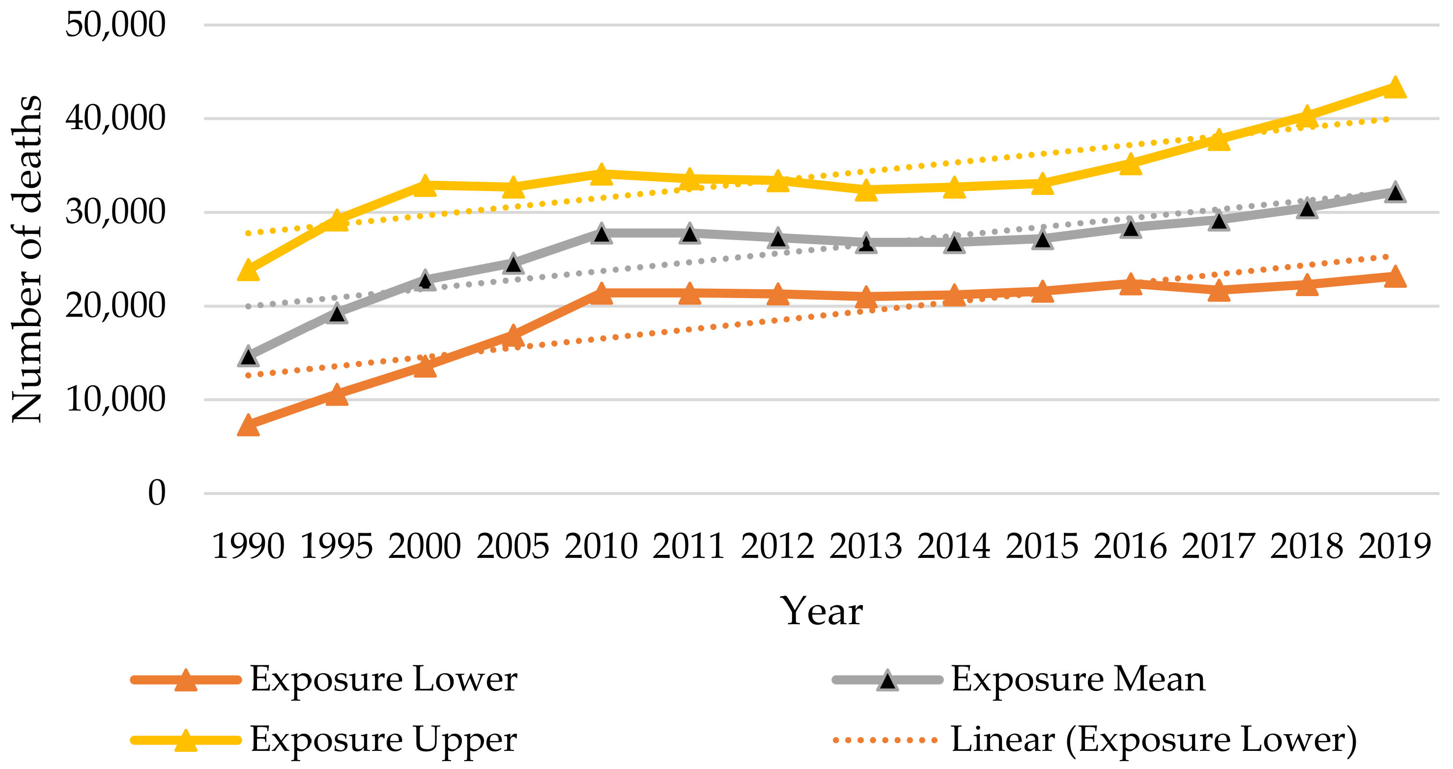
The Health Effects Institute [5] presented the increasing number of deaths attributable to PM2.5 in a given year as those deaths that had occurred earlier than would have been expected in the absence of PM2.5, which was computed based on nonlinear integrated-exposure-response (IER) functions, for all ages and sexes combined between 1990 and 2019 in Thailand. These data are presented in Figure 1. However, Apte et al. [6] suggested that exposure to ambient fine particulate matter (PM2.5) air pollution was a significant risk for premature death. However, if PM2.5 in all countries met the WHO’s air quality guideline (10 µg/m³), the estimated life expectancy could increase by a population-weighted median of 0.6 years (interquartile range of 0.2–1.0 years).

Ambient air pollutants include particulate matter (PM), ozone, nitrogen dioxide, sulfur dioxide, and other contaminants. PM is a complex mixture of solid and liquid particles of primary and secondary origin, and contains a wide range of inorganic and organic components. PM mass and composition are also highly variable in spatiotemporal terms and are strongly influenced by climatic and meteorological conditions [7]. PM can be emitted from natural and human-made sources, including forest fires, dust storms, traffic, and industry.

Basically, PM is measured as particles with an aerodynamic diameter of less than 10 μm (PM10) and less than 2.5 μm (PM2.5) [8]. Particles at PM10 are inhalable and may reach the upper part of the airways and lungs, while smaller PM2.5 particles are more able to penetrate the lungs and perhaps reach the alveoli. Ultrafine particles, which have a cut-off at 0.1 μm, may be a small proportion of the total mass but may also have the most significant health impacts due to their ability to pass from the lung directly into the bloodstream and their larger reactive surface area, which may be capable of inducing more significant damage [7].

PM exposure depends on physical characteristics, including breathing mode, rate, and volume of a person’s lungs; particle size has been linked as a leading cause of health problems. Generally, the smaller a particle is, the more deeply and rapidly it can penetrate and deposit on the respiratory tract. In nasal breathing, the cilia and the mucus together act as an active filter for most particulates exceeding 10 μm, or coarse PM. As the coarse PM fraction settles quickly, it tends to lodge in the upper throat or the bronchi. If humans inhale this PM, it will be initially collected in the nose and throat. The body will then react to eliminate these intruding PMs through sneezing and coughing [9].

Furthermore, many researchers studied the effects of air pollution, including PM, on the materials. Varotsos and Cartalis [10] stated that atmospheric pollution accelerates the material deterioration of buildings and other structures and objects of cultural heritage. The corrosive effects of gaseous SO₂, NO_x, O₃, HNO₃, PM, and acid rainfall in combination with climatic parameters are crucial, especially for mega-cities such as Athens with unique historic monuments ([10,11]). Tzanis et al. [12] reported nitric acid and particulate matter measurements in Athens, Greece.

In Thailand, PM has had diverse and far-reaching effects on the economy, impacting tourism, property values, and medical treatment costs. According to the Kasikorn Research Centre report in 2019, the smog could cost Thailand THB 6.6 billion in losses due to air pollution in the healthcare and tourism sectors [13]. The Thai Public Broadcasting Service reported the effect of PM2.5 on medical expenses and the loss of tourism opportunities in and around Bangkok if PM2.5 does not ease within a month: Medical expenses per person could reach an average of THB 1000 for each medical visit and THB 22.50 per day for face masks. Total medical costs alone could be in the range of THB 1.6–3.1 million, depending on the intensity of the air pollution [14].

Therefore, the monitoring of PM10 and PM2.5 should be improved in many countries to assess population exposure and to encourage local authorities to improve air quality [15]. However, most pollutant concentration information has been obtained from ground monitoring stations, which have significant limitations: limited in number, unequally distributed, and varied measure frequency ranges. These can affect the geographical and demographic range of studies, resulting in an information bias and a lack of exposure–response studies [2].

The spatiotemporal variations of PM10 and PM2.5 are complex, and continuous monitoring is not possible in many countries and regions. Therefore, satellite-based remote sensing has become a widely used technique for monitoring. It can provide extensive spatial coverage and is cost-effective for studies. In addition, the data is acquired directly from the measured spectral aerosol optical depth (AOD), which is the integration of aerosol light extinction across a vertical path through the atmosphere [16]. However, atmospheric aerosols are a complex mixture of particles (being ubiquitous in air, often observable as dust, smoke, and haze) arising from a large number of discrete natural and anthropogenic sources (e.g., Ondov and Wexler [17]; Murr and Garza [18]; Varotsos and Zellner [19]; Varotsos et al. [20]).

Therefore, a suitable model for spatiotemporal PM concentration prediction in rural and urban landscapes was investigated based on the review article of Chu et al. [2], “A Review on Predicting Ground PM2.5 Concentration Using Satellite Aerosol Optical Depth.” They found that four predicting models were widely used: multiple linear regression (MLR), mixed-effect model (MEM), chemical transport model (CTM) and geographically weighted regression (GWR). Regarding the prediction accuracy, MEM performs the best, while MLR performs the worst. CTM predicts PM2.5 better on a global scale, while GWR performs well on a regional level. Therefore, MEM and GWR models were chosen to examine a suitable model for spatiotemporal PM concentration prediction in rural and urban landscapes. Consequently, spatiotemporal PM concentration predictions using a moderate resolution imaging spectroradiometer (MODIS) AOD with significant PM factors in rural and urban landscapes in Thailand are necessary due to the limitations of PM monitoring stations.

The expected results provide significant spatiotemporal data affecting PM10 and PM2.5 concentrations in rural and urban landscapes. The results can also provide the spatial patterns of PM10 and PM2.5 concentrations in both landscapes at the district level in the winter and summer seasons. Additionally, the results can be used as guidelines for improving air quality and reducing impacts on human health. The objective of this research was to predict spatiotemporal PM10 and PM2.5 concentrations in rural and urban regions during the winter and summer seasons. The specific research concerns were (1) to identify significant factors of PM10 concentrations in rural regions and PM2.5 concentrations in urban landscapes in the winter and summer seasons as well as their interrelationships using the multicollinearity test and an ordinary least squares (OLS) regression analysis; (2) to predict spatiotemporal PM10 and PM2.5 concentrations using GWR and MEM models, and (3) to evaluate a suitable spatiotemporal model for PM10 and PM2.5 concentration prediction and validation.

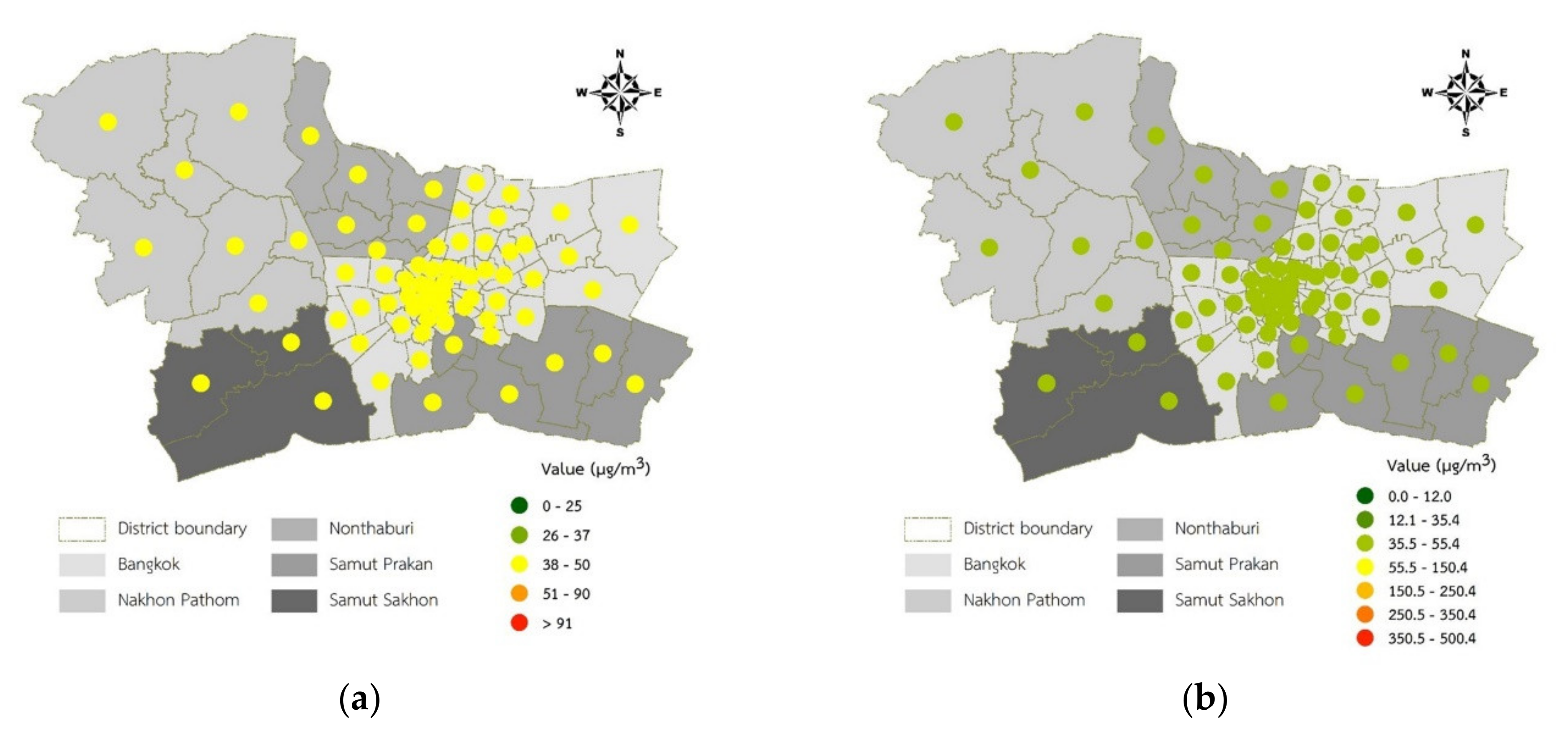
2. Study Area

Two study areas were chosen for two different studies affecting PM10 concentrations in rural landscapes and PM2.5 concentrations in urban landscapes, as shown in Figure 2. We chose rural and urban landscapes according to recent land use data from Thailand’s Land Development Department [21].

According to the Land Development Department [21], more than 65 percent of rural landscapes, which covers approximately 15,827 sq km with 60 districts from 6 provinces (i.e., Ang Thong, Lop Buri, Phra Nakhon Si Ayutthaya, Pathum Thani, Saraburi, and Sing Buri) are agricultural, including features such as paddy fields, field crops, orchards, and perennial trees. Agricultural operations, mainly agricultural debris burning, generate massive sources of PM10 contribution. Arslan and Aybek [22] stated that agricultural field operations caused dust production in conventional crop production, including soil tillage and seedbed preparation, planting, fertilization, pesticide application, harvesting, and post-harvest processes. The high PM10 concentration distribution in the dust is circulated and spread by the wind, especially on the surfaces without cement and asphalt [23].

Meanwhile, urban landscapes cover approximately 6180 sq km with 72 districts from 5 provinces, including Bangkok, Nakhon Pathom, Nonthaburi, Samut Prakan, and Samut Sakhon. This landscape, especially in Bangkok, the capital city of Thailand, has a high-density population and economic activity clusters. Lin et al. [24] stated that high PM2.5 concentrations have primarily been identified in regions with high populations, rapid urban expansion, and local economic growth.

3. Material and Method

The overview framework of the research methodology consisted of four components, including (1) data collection and preparation; (2) identification of significant spatiotemporal factors affecting PM concentrations; (3) prediction of spatiotemporal PM concentrations, and (4) a suitable spatiotemporal model for PM concentration prediction and validation, as shown in Figure 3. Details of each stage are separately described in the following sections.

3.1. Data Collection and Preparation

Data included ground-level PM data, as dependent variables, and meteorological, biophysical, and socioeconomic data, as independent variables, from October 2019 to May 2020, that were collected from national and international organizations and then prepared using standard tools in the Environmental Systems Research Institute (ESRI) ArcMap software, as summarized in

Table 1. List of data collection and preparation for analysis and modeling in the study.

Categories	Variables	Source	Time-Frequency	Data Preparation
PM data at ground level	PM10	PCD BMA	Daily Daily	Optimal interpolation method
	PM2.5	PCD BMA	Daily Daily
Meteorological data	Relative humidity (RH)	TMD	Daily	Optimal interpolation method
	Temperatures (TEMP)	TMD	Daily
	Wind speed (WS)	TMD	Daily
	Pressure (P)	TMD	Daily
	Visibility (VIS)	TMD	Monthly
Biophysical data	MCD19A2 (AOD)	USGS	Daily	Raster calculator
	NDVI	USGS	Seasonal	Raster calculator from Landsat 8 operational land imager (OLI) data
	BUI	USGS	Seasonal
	Road density (RD)	MOT	-	Calculate geometry and field calculator
	Factory density (FD)	DIW	-	Spatial join and field calculator
	Elevation (ELEV)	USGS	-	Fill (spatial analysis) from shuttle radar topography mission (SRTM) data
	Brightness temperature (BT)	NASA	daily	Optimal interpolation method
	Fire radiative power (FRP)	NASA	daily
	Fire hotspot (FH)	NASA	daily	Spatial join and field calculator
Socioeconomic data	Population density (POP)	NSO	Yearly	Field calculator (extract from population data at district level)
	Gross provincial product (GPP)	NESDC	Yearly

Note: BMA: Bangkok Metropolitan Administration; DIW: Department of Industrial Works; MOT: Ministry of Transport; NASA: NASA’s Earth Science Data Systems; NSO: National Statistical Office; NESDC: Office of the National Economic and Social Development Council; PCD: Pollution Control Department; TMD: Thai Meteorological Department; USGS: United States Geological Survey.

.

In this study, available interpolation methods under the ESRI ArcMap software, which many researchers use, were examined to identify an optimal method for specific factors. Seven interpolation methods, namely inverse distance weighted (IDW), global polynomial interpolation (GPI), radial basis functions (RBF), ordinary kriging (OK), ordinary cokriging (OCK), simple kriging (SK), and simple cokriging (SCK), were selected to examine an optimal interpolation method for appropriate dependent and independent variables, including average monthly PM data at ground level, meteorological data (e.g., relative humidity, temperature, wind speed, pressure, visibility), and MODIS fire data (e.g., brightness temperature and radiative firepower) based on the existing data between October 2019 to May 2020 using the average monthly root mean squared error (RMSE) from each method. The RMSE indicates how closely a model predicts measured values. The RMSE value was derived using the following equation:

$$\mathrm{RMSE}=\sqrt{\frac{{{\displaystyle \sum }}_{\mathrm{i}=1}^{\mathrm{n}}{\left(\mathrm{predicted} - \mathrm{measured}\right)}^2}{\mathrm{n}}}$$

(1)

where n is the number of measured data.

However, appropriate standard tools for the Spatial Analyst tool in ESRI ArcMap software were applied with other independent variables, including MODIS AOD, normalized difference vegetation index (NDVI), built-up index (BUI), road density, factory density, elevation, fire hotspot, population density, and gross provincial product (GPP).

After that, all prepared variables were normalized using the Z-score method to identify significant spatiotemporal factors in PM concentrations in the next stage.

In practice, mean and standard deviation values at the district level of all dependent and independent variables were first extracted using the zonal statistics analysis. Then, they were exported into Microsoft Excel spreadsheets and normalized using the Z-score method as follows:

$$\mathrm{Z}=\frac{(\mathrm{X} - \mathsf{\mu })}{\mathsf{\sigma }}$$

(2)

where Z is the standard score, X is the observed value, μ is the mean of the sample, and σ is the standard deviation of the sample. As a result, the mean values of all variables are zero, and their standard deviation values are one.

3.2. Identification of Significant Spatiotemporal Factors Affecting PM Concentrations and Relationships

Normalized dependent and independent variables affecting PM10 concentrations in rural landscapes and PM2.5 concentrations in urban landscapes in the winter (October 2019–February 2020) and summer (March 2020–May 2020) were applied to identify significant spatiotemporal factors using the multicollinearity test with a variance inflation factor (VIF) and the OLS regression analysis.

VIF measures the amount of multicollinearity in a set of multiple regression variables. A high VIF value indicates that the associated independent variable is redundant with the other variables in the model. Therefore, the VIF value should be lower than 7.5 to avoid multicollinearity, as suggested in ArcGIS 10.3.1 documentation [25], as follows:

$${\mathrm{VIF}}_{\mathrm{i}}=\frac{1}{ 1 -{ \mathrm{R}}_{\mathrm{i}}^2}$$

(3)

where R_i² comprises multiple coefficients of determination in a regression of the ith predictor on the others.

The main output of the OLS regression analysis was the significant spatiotemporal factors affecting PM10 concentrations in rural landscapes and PM2.5 concentrations in urban landscapes in the winter and summer seasons.

3.3. Prediction of Spatiotemporal PM Concentrations

Under this component, primary input data (MODIS AOD) and significant spatiotemporal independent variables (the output from component 1) affecting PM10 and PM2.5 concentrations in the rural and urban landscapes, respectively, were separately applied to predict monthly PM concentrations in winter and summer seasons using the GWR and MEM models.

In this study, the standard function of the GWR model (as a local model) with an adaptive kernel type and AICc bandwidth was applied to predict PM concentrations in the ESRI ArcMap software environment. The efficiency of the GWR model was automatically reported using the corrected Akaike information criterion (AICc), coefficient of determination (R²), and adjusted R-squared (${\overline{\mathrm{R}}}^2$) using the following equations:

$$\mathrm{AICc}=\left(-2\log \left(\mathrm{L}\right) +2\mathrm{k}\right)+\frac{2\mathrm{k}(\mathrm{k}+1)}{\mathrm{n} - \mathrm{k} - 1}$$

(4)

$${\mathrm{R}}^{2 }=1 -\frac{{\mathrm{SS}}_{\mathrm{res}}}{{\mathrm{SS}}_{\mathrm{tot}}}$$

(5)

$${\overline{\mathrm{R}}}^2=1 -\frac{\raisebox{1ex}{${\mathrm{SS}}_{\mathrm{res}}$}\!\left/ \!\raisebox{-1ex}{$(\mathrm{n} - \mathrm{k})$}\right.}{ \raisebox{1ex}{${\mathrm{SS}}_{\mathrm{tot}}$}\!\left/ \!\raisebox{-1ex}{$(\mathrm{n} - 1)$}\right.}$$

(6)

Here, L is the maximum likelihood for the estimated model, k is the number of independent variables, n is the number of sample sizes, ${\mathrm{SS}}_{\mathrm{res}}$ is the sum of squares of residual or called the residual sum of squares, and ${\mathrm{SS}}_{\mathrm{tot}}$ is the total sum of squares.

Meanwhile, the MEM model (as a global model) with fixed effects intercepts and scaled identity covariance type was applied to predict PM concentrations using the IBM SPSS statistics software. The efficiency of the models was automatically reported using the AIC, corrected Akaike information criterion (AICc), and Bayesian information criterion (BIC) as follows:

$$\mathrm{AIC}=-2\log \left(\mathrm{L}\right)+2\mathrm{k}$$

(7)

$$\mathrm{BIC}=-2\log \left(\mathrm{L}\right)+\mathrm{klog}\left(\mathrm{N}\right)$$

(8)

where $\log \left(\mathrm{L}\right)$ is the value of the log-likelihood function of the fitted model evaluated at the model estimate, k is the number of fitted model parameters, and N is the recorded measurements.

The results of this analysis were the monthly and seasonally predictive equations for monthly PM10 concentrations in rural landscapes and PM2.5 concentrations in urban landscapes during the winter and summer seasons. Additionally, the air quality index (AQI), based on the monthly PM10 concentrations in rural landscapes and PM2.5 concentrations in urban landscapes over two seasons, and according to Thailand and the U.S. EPA AQI standards, was mapped (see

Table 2. Thailand’s air quality index classification based on affected PM concentrations.

Level of Thai AQI	PM10 (µg/m3)	PM2.5 (µg/m3)	Meaning
1	0–50	0–25	Excellent
2	51–80	26–37	Satisfactory
3	81–120	38–50	Moderate
4	121–180	51–90	Unhealthy
5	>181	>91	Very unhealthy

Source: Pollution Control Department [26].

and

Table 3. The U.S. EPA air quality index classification based on affected PM concentrations.

Level of AQI	PM10 (µg/m3)	PM2.5 (µg/m3)	Meaning
1	0–54	0.0–12.0	Good
2	55–154	12.1–35.4	Moderate
3	155–254	35.5–55.4	Unhealthy for sensitive groups
4	255–354	55.5–150.4	Unhealthy
5	355–424	150.5–250.4	Very unhealthy
6	425–504	250.5–350.4	Hazardous
7	505–604	350.5–500.4

Source: U.S. Environmental Protection Agency [27].

).

3.4. Suitable Spatiotemporal Model for PM Concentration Prediction and Validation

Under this component, a suitable model for spatiotemporal PM10 and PM2.5 concentration predictions between GWR and MEM models was first identified based on their AICc values. (See also Section 3.3). In general, a lower AICc value indicates a better fit model. In practice, average AICc values for PM10 concentrations in rural landscapes, and PM2.5 concentrations in urban landscapes in winter and summers from GWR and MEM models, were calculated to identify a suitable model for spatiotemporal PM10/PM2.5 concentration predictions.

Furthermore, a suitable model for spatiotemporal PM10 and PM2.5 concentration predictions was validated with a new dataset (October 2020–May 2021) using Pearson’s correlation analysis. The expected correlation coefficient value should be equal to or more than 0.5, which indicates a strong linear relationship between the dependent and independent variables [28].

4. Results and Discussion

4.1. Optimal Method for a Specific Variable Identification

The optimal methods for monthly mean PM10 concentrations, PM2.5 concentrations, relative humidity, temperature, wind speed, pressure, visibility, brightness temperature, and radiative firepower interpolation with seven different methods (i.e., IDW, GPI, RBF, OK, OCK, SK, and SCK) based on the average RMSE value under cross-validation are summarized below.

4.1.1. PM10 and PM2.5 Concentrations

The SCK method with either the hole effect or the K-Bessel function could have been used as an optimal method for monthly mean PM10 concentration interpolation since both functions could provide the lowest RMSE value. As a result, the average RMSE value of monthly mean PM10 concentration interpolation was 15.73 µg/m³. The SCK method with the K-Bessel function was chosen as an optimal method for monthly mean PM2.5 concentration interpolation. The average RMSE value of monthly mean PM2.5 concentration interpolation was 15.73 µg/m³. Nevertheless, previous research on a suitable interpolation method for predicting PM10 and PM2.5 concentrations at international and national levels reported success using different methods.

Sajjadi et al. [29] selected four interpolation methods (i.e., IDW, RBF, OK, and UK) to identify an optimal method for predicting PM10 and PM2.5 in Sabzevar City in the Razavi Khorasan Province, Iran, using RMSE, MAE, and MAPE. They found that IDW was the best interpolation method for PM10 and PM2.5 concentration predictions. Meanwhile, Vorapracha et al. [30] selected three methods (i.e., IDW, OK, and UK) to identify a suitable method for predicting PM10 in the central region of Thailand using RMSE. They also found that the most suitable method for PM10 prediction was IDW. Meanwhile, Wong et al. [31] identified OK as a suitable method for PM10 prediction compared to IDW. Likewise, Kumar et al. [32] reported OK as the best interpolation method for PM10 concentration prediction among the three selected methods (i.e., IDW, OK, and spline).

As compared to previous studies, we examined more interpolation methods with various functions to ensure the accuracy and efficiency of our results. After considering seven different methods, namely IDW, GPI, RBF, OK, OCK, SK, and SCK, for use with RMSE, we selected the SCK method, as it applies the covariance between two or more realizations of cross-correlated random fields [33], which would be the most suitable for our research objectives.

4.1.2. Relative Humidity

The SCK method with the J-Bessel function was selected as an optimal method for monthly mean relative humidity interpolation. The average RMSE value of monthly mean relative humidity interpolation was 3.43%.

4.1.3. Temperature

The SCK method with the hole effect function is selected as an optimal method for monthly mean temperature interpolation. The average RMSE value of monthly mean temperature interpolation was 0.79 degrees Celsius.

4.1.4. Wind Speed

The RBF method, with the spline with tension and one sector, was chosen as an optimal method for monthly mean wind speed interpolation. The average RMSE value of monthly mean wind speed interpolation was 1.54 knots.

4.1.5. Pressure

The SCK method with the stable function was selected as an optimal method for monthly mean pressure interpolation. The average RMSE value of monthly mean pressure interpolation was 0.40 hPa.

4.1.6. Visibility

The OCK method with the hole effect function was selected as an optimal method for monthly mean visibility interpolation. The average RMSE value of monthly mean visibility interpolation was 1.32 km.

As reported in Section 4.1.2, Section 4.1.3, Section 4.1.4, Section 4.1.5 and Section 4.1.6, the average RMSE values from the seven interpolation methods of monthly mean meteorological data were similar. In the meantime, the previous studies on a suitable interpolation method for predicting monthly mean meteorological data at international and national levels have reported different methods. Prasomsup [34] found that the SCK was the optimal method for monthly mean temperatures in November, December, February, and March, while OCK was optimal in January and April. Jantakat and Ongsomwang [35] selected OCK for interpolated monthly mean temperatures in January, November, and December, while they selected Distinctive Cokriging (DCK) for February–October. At the same time, Ozturk and Kilic [36] chose OK for interpolated temperature and precipitation during 5-year periods. Similar to what Cao et al. [37] presented, the OK with exponential and spherical had the best interpolation precision.

Likewise, as Keskin and Özdoğu [38] presented, OK performed better overall than the other interpolation methods for wind speed data. In contrast, this study suggested RBF with spline with tension functions; the geometry of the search neighborhood was an ellipse. We followed the study of Gradka and Kwinta [39]. The RBF was conceptually similar to fitting a rubber membrane through the measured sample values while minimizing the surface’s total curvature and selecting one functional parameter to control the surface’s smoothness using cross-validation. In addition, the RBF represented an irregular surface using many linear functions that connected the node with the data point and could be an alternative to kriging.

Equally, the other techniques could be used to interpolate meteorological data. However, the most commonly used have been the kriging technique and the additions of the cross-correlated variables to reduce the estimation error variance [40]. However, Kuo et al. [41] used the kriging method to interpolate the temperature data with a focus on the optimal sample size of the sensors. In addition, Deligiorgi and Philippopoulos [42] reported that the most common kriging method was simple kriging, which assumes a known constant mean, as compared to ordinary kriging, which assumes an unknown constant mean. As well, kriging is also known as the best unbiased linear estimator.

Many suitable interpolation methods are possible for predicting monthly mean meteorological data; the method selected should be based on the objective and parameters involved in the research, as mentioned in Section 4.1.1.

4.1.7. MODIS Brightness Temperature

The SCK method with the stable function was selected as an optimal method for monthly mean brightness temperature interpolation. The average RMSE value of monthly mean brightness temperature interpolation was 4.56 degrees Kelvin.

4.1.8. MODIS Fire Radiative Power

The RBF method with the spline with tension and eight sector functions was selected as an optimal method for monthly mean fire radiative power interpolation. The average RMSE value of monthly mean fire radiative power interpolations was 19.44 MW.

Several methods were used to interpolate MODIS fire data from previous studies. For example, Veraverbeke et al. [43] used kriging for interpolating the MODIS active fire as kriging is based on local variogram analysis and allows uncertainty analysis by spatially estimating the kriging standard error. Similar to Devkota [44], Ponomarev et al. [45] used kriging to interpolate the MODIS fire radiative power data. Loboda et al. [46] used IDW to determine the fire spread from MODIS active fire points data.

As discussed in Section 4.1.1, Section 4.1.2, Section 4.1.3, Section 4.1.4, Section 4.1.5 and Section 4.1.6, the rationale for a suitable interpolation method for predicting monthly mean MODIS fire data should be based on the research objective and required parameters.

4.2. Suitable Method for Specific Factors Preparation

Standard tools under ESRI ArcMap software were applied to prepare other independent variables, including MODIS AOD, NDVI, BUI, road density, factory density, elevation, fire hotspot, population density, and GPP, as summarized in

Table 4. Summary of the standard tools for other independent variable preparation.

No.	Variable	Data Preparation
1	MODIS AOD	Raster calculator
2	NDVI	Raster calculator from Landsat 8 OLI data
3	BUI	Raster calculator from Landsat 8 OLI data
4	Road density	Calculate geometry and field calculator
5	Factory density	Spatial join and field calculator
6	Elevation	Fill (spatial analysis) from SRTM data
7	Fire hotspot	Spatial join and field calculator
8	Population density	Field calculator (extract from population data at district level)
9	Gross provincial product	Field calculator (extract from population data at district level)

.

All prepared dependent and independent variables with Z-score normalization were further applied to identify significant spatiotemporal factors affecting PM concentrations using the multicollinearity test and the OLS regression analysis.

4.3. Significant Spatiotemporal Factors Affecting PM10 Concentrations in Rural Landscapes

The multicollinearity test of independent factors affecting PM10 concentrations after normalization is reported in

Table 5. Multicollinearity test of explanatory variables for PM10 concentrations.

No.	Variable	The VIF Value
		Winter Season					Summer Season
		Oct 2019	Nov 2019	Dec 2019	Jan 2020	Feb 2020	Mar 2020	Apr 2020	May 2020
1	RH	5.50	4.84	22.76 *	44.83 *	22.93 *	22.23 *	38.47 *	15.69 *
2	TEMP	2.22	2.95	3.35	2.64	1.83	4.16	23.13 *	6.06
3	WS	4.54	3.81	4.01	16.13 *	5.85	8.43 *	9.10 *	8.12 *
4	P	2.65	6.46	7.24	63.79 *	8.65	5.42	2.42	4.96
5	VIS	3.05	3.90	3.66	9.76 *	5.03	6.62	3.93	4.51
6	AOD	4.61	2.49	3.48	6.35	2.63	2.15	3.99	2.47
7	NDVI	20.14 *	24.17 *	22.76 *	18.97 *	18.65 *	18.64 *	18.70 *	22.42 *
8	BUI	25.74 *	29.89 *	24.22 *	24.66 *	21.81 *	16.76 *	15.52 *	17.86 *
9	RD	12.18 *	13.25 *	12.05 *	11.97 *	10.92 *	11.41 *	15.53 *	15.58 *
10	FD	5.63	5.60	6.94	6.61	6.80	4.77	5.87	4.96
11	BT	3.47	3.00	3.07	2.87	1.63	7.33	4.32	1.30
12	FRP	1.92	2.76	2.94	3.34	3.22	2.70	3.62	4.04
13	FH	1.49	1.63	1.73	1.65	1.54	2.10	1.79	2.05
14	ELEV	3.50	3.54	4.74	5.58	4.22	4.14	5.73	3.98
15	POP	11.58 *	10.21 *	12.49 *	13.39 *	12.44 *	10.53 *	13.35 *	11.23 *
16	GPP	5.66	4.50	4.36	4.72	5.02	5.21	5.18	4.62
Total uncorrelated factors		12	12	11	8	10	10	9	10

Note: * These factors are excluded for significant factor identification since the VIF value is equal to or more than 7.5 for the OLS regression analysis.

. The results showed that the uncorrelated factors varied by 8–10 factors per month. In addition, NDVI, BUI, road density, and population density were redundant in PM10 concentrations every month. Therefore, the next step would exclude the correlated factors with a VIF value equal to or more than 7.5 for the OLS regression analysis.

The results of the OLS regression analysis for significant factors in PM10 concentrations identification are summarized in

Table 6. Monthly and seasonally significant factors affecting PM10 concentrations.

No.	Candidate Factors	Significant Factors Affecting PM10 Concentrations
		Winter Season					Summer Season
		Oct 2019	Nov 2019	Dec 2019	Jan 2020	Feb 2020	Mar 2020	Apr 2020	May 2020
1	RH	N.S.	N.S.	N.A.	N.A.	N.A.	N.A.	N.A.	N.A.
2	TEMP	TEMP *	N.S.	TEMP *	TEMP *	N.S.	TEMP *	N.A.	N.S.
3	WS	WS *	WS *	WS *	N.A.	WS *	N.A.	N.A.	N.A.
4	P	N.S.	N.S.	N.S.	N.A.	N.A.	N.S.	N.S.	N.S.
5	VIS	VIS *	VIS *	VIS *	N.A.	N.S.	N.S.	N.S.	VIS *
6	AOD	N.S.	AOD *	N.S.	AOD *	N.S.	AOD *	N.S.	N.S.
7	FD	N.S.	N.S.	N.S.	N.S.	N.S.	FD *	N.S.	N.S.
8	BT	N.S.	N.S.	N.S.	N.S.	N.S.	N.S.	BT *	N.S.
9	FRP	N.S.	N.S.	N.S.	N.S.	FRP *	N.S.	N.S.	N.S.
10	FH	N.S.	N.S.	N.S.	N.S.	N.S.	N.S.	N.S.	N.S.
11	ELEV	N.S.	N.S.	N.S.	N.S.	N.S.	N.S.	N.S.	N.S.
12	GPP	N.S.	N.S.	N.S.	N.S.	N.S.	N.S.	N.S.	N.S.
Total significant factors		3	3	3	2	2	3	1	1

Note: N.A. indicates not applied after multicollinearity test, * indicates significant at the confident level of 99% using OLS regression analysis, and N.S. indicates not significant at the confident level of 99% using OLS regression analysis.

. The results indicated significant differences among the monthly factors for PM10 concentrations. The number of significant factors affecting PM10 concentrations in winter and summer was five each season, and they varied per season. Three common factors impacting PM10 concentrations were temperature, visibility, and MODIS AOD that were identified in both seasons. Two significant factors affecting PM10 concentrations only found during the winter season included wind speed and fire radiative power. In contrast, factory density and brightness temperature were the only factors during the summer season. These findings indicated that factory density (FD) related to human activity in April might be managed to reduce the impact on PM10 concentrations in rural landscapes.

The significant factors affecting PM10 concentrations in this study were similar to those found in a previous study by Harnkijroong and Panich [47]. They reported that PM10 concentrations on the roadsides of Bangkok were most relevant to the temperature, followed by the wind speed. They also found that rainfall did not influence PM10 concentrations.

Furthermore, Unal et al. [48] suggested that PM10 concentrations were associated with wind speed, and high PM10 concentrations were found in high pressure and low wind speed. Likewise, the most significant meteorological factors, including planetary boundary layer height, temperature, wind speed, and precipitation influenced by the seasonal dynamics of PM10 concentrations, were reported by Czernecki et al. [49].

In addition, many studies reported the relationship between MODIS AOD and PM10 concentrations [50,51,52,53]. Ferrero et al. [51] found a strong relationship between the two and developed a high accuracy algorithm to predict ground PM concentrations based on AOD mixing height and wind speed. Similarly, Kanabkaew [53] reported that the relationship between AOD and hourly PM improved accuracy when corrected with meteorological factors, including relative humidity and temperature data.

4.4. Significant Spatiotemporal Factors Affecting PM2.5 Concentrations in Urban Landscapes

The multicollinearity test of independent factors affecting PM2.5 concentrations after normalization in urban landscapes in the winter and summer seasons is reported in

Table 7. Multicollinearity test of explanatory variables affecting PM2.5 concentrations.

No.	Variable	The VIF Value
		Winter Season					Summer Season
		Oct 2019	Nov 2019	Dec 2019	Jan 2020	Feb 2020	Mar 2020	Apr 2020	May 2020
1	RH	11.88 *	6.51	15.56 *	25.58 *	2.50	20.80 *	16.97 *	41.35 *
2	TEMP	11.69 *	9.87 *	28.18 *	7.19	9.30 *	5.47	13.14 *	9.45 *
3	WS	4.03	4.81	4.83	4.94	3.38	6.10	4.46	4.24
4	P	7.11	8.70 *	16.09 *	26.68 *	6.10	17.24 *	16.03 *	38.35 *
5	VIS	2.11	1.86	6.65	4.26	1.46	2.19	3.62	6.06
6	AOD	2.41	2.43	8.33 *	5.60	2.07	1.50	2.82	2.47
7	NDVI	42.06 *	48.43 *	75.04 *	73.29 *	48.76 *	24.12 *	32.56 *	27.57 *
8	BUI	76.13 *	79.61 *	105.99 *	110.25 *	88.86 *	38.65 *	49.40 *	42.13 *
9	RD	20.30 *	15.60 *	16.47 *	16.43 *	17.19 *	14.29 *	16.94 *	13.31 *
10	FD	2.88	2.59	2.63	4.12	2.88	2.51	3.55	2.62
11	BT	2.39	1.56	13.88 *	8.11 *	3.55	3.48	2.68	2.96
12	FRP	4.13	4.28	7.87 *	5.12	3.55	4.50	6.25	5.90
13	FH	2.07	1.25	2.42	2.20	1.18	2.10	1.45	1.91
14	ELEV	5.89	5.29	5.73	5.49	5.83	5.46	6.19	5.11
15	POP	44.96 *	38.81 *	46.98 *	36.86 *	37.13 *	28.17 *	25.59 *	30.01 *
16	GPP	28.92 *	30.98 *	36.30 *	27.77 *	25.59 *	19.19 *	20.42 *	18.67 *
Total uncorrelated factors		9	9	5	8	10	9	8	8

Note: * These factors are excluded for significant factor identification in the OLS regression analysis.

. The uncorrelated factors varied by 5–10 factors per month. In addition, NDVI, BUI, road density, population density, and GPP were redundant with PM2.5 concentrations every month. Therefore, the next step would exclude the correlated factors with a VIF value equal to or more than 7.5 in the OLS regression analysis.

The results of the OLS regression analysis for significant factors affecting PM2.5 concentration identification are summarized in

Table 8. Monthly and seasonally significant factors affecting PM2.5 concentrations.

No.	Candidate Factors	Significant Factors Affecting PM2.5 Concentrations
		Winter Season					Summer Season
		Oct 2019	Nov 2019	Dec 2019	Jan 2020	Feb 2020	Mar 2020	Apr 2020	May 2020
1	RH	N.A.	N.S.	N.A.	N.A.	RH *	N.A.	N.A.	N.A.
2	TEMP	N.A.	N.A.	N.A.	TEMP *	N.A.	N.S.	N.A.	N.A.
3	WS	WS *	N.S.	WS *	N.S.	WS *	N.S.	WS *	WS *
4	P	P *	N.A.	N.A.	N.A.	P *	N.A.	N.A.	N.A.
5	VIS	VIS *	VIS *	VIS *	VIS *	N.S.	N.S.	VIS *	VIS *
6	AOD	AOD *	N.S.	N.A.	AOD *	N.S.	N.S.	AOD *	N.S.
7	FD	N.S.	N.S.	N.S.	N.S.	N.S.	N.S.	FD *	FD *
8	BT	BT *	N.S.	N.A.	N.A.	N.S.	N.S.	BT *	BT *
9	FRP	FRP *	FRP *	N.A.	N.S.	FRP *	FRP *	FRP *	N.S.
10	FH	FH *	N.S.	N.S.	FH *	N.S.	N.S.	FH *	N.S.
11	ELEV	ELEV *	N.S.	N.S.	ELEV *	ELEV *	N.S.	N.S.	ELEV *
Total significant factors		8	2	2	5	5	1	7	5

Note: N.A. indicates not applied after multicollinearity test, * indicates significant at the confident level of 99% using OLS regression analysis, and N.S. indicates not significant at the confident level of 99% using OLS regression analysis.

. The significant factors affecting PM2.5 in winter and summer were ten and eight, respectively. Many meteorological factors significantly influenced PM2.5, as compared to PM10 concentrations [54]. This study found seven common factors affecting PM2.5 concentrations in both seasons: wind speed, visibility, brightness temperature, fire radiative power, MODIS AOD, fire hotspot, and elevation. Three significant factors affecting PM2.5 concentrations were only found in the winter season: relative humidity, temperature, and pressure. In contrast, one significant factor affecting PM2.5 concentrations, factory density, was only identified in the summer season. These findings imply that factory density (FD), MODIS brightness temperature (BT), MODIS fire radiative power (FRP), and MODIS fire hotspot (FH) factors that are related to human activities which are found in a specific month might be managed to reduce the impact on PM2.5 concentrations.

The findings showed similar results to the previous study of Guo and Zhang [55], who had reported that PM2.5 concentrations were most relevant to visibility, followed by wind speed. The least pertinent factors were temperature and relative humidity. Likewise, these findings were consistent with Chen et al. [54], who showed the strong influence of wind speed on local PM2.5 concentrations. They also observed strong interactions between wind speed and other meteorological factors influencing PM2.5 concentrations. Galindo et al. [56] found that the winter wind speed was the main influence on the dilution of atmospheric aerosols, while temperature and solar radiation strongly influenced coarser particles. This indicated that the meteorological data and the solar heating at the Earth’s surface via the active fire data were significantly related to PM2.5 concentrations. In addition, MODIS AOD had a strong correlation to PM2.5 concentrations [57,58]. Similarly, Lee et al. [59] reported potentially helpful methods for predicting PM2.5 concentrations. Chudnovsky et al. [60] predicted PM2.5 concentrations with MODIS AOD and improved the accuracy when land use and meteorological data were included. However, Chu et al. [2] suggested using AOD data with higher resolution to obtain a more accurate estimation of PM2.5 concentrations in relatively small areas.

4.5. Prediction of PM10 Concentrations in Rural Landscapes Using GWR and MEM Models

The generic equations for PM10 concentrations in winter and summer in rural landscapes using the GWR model as a local model are shown in Equations (9) and (10):

$${\mathrm{y}}_{(\mathrm{i},\mathrm{j})}=\beta {\mathrm{o}}_{\mathrm{i},\mathrm{j}}+ \beta {\mathrm{k}}_{1(\mathrm{i},\mathrm{j})}\mathrm{TEMP}+ \beta {\mathrm{k}}_{2(\mathrm{i},\mathrm{j})}\mathrm{WS}+\beta {\mathrm{k}}_{3(\mathrm{i},\mathrm{j})}\mathrm{VIS}+\beta {\mathrm{k}}_{4(\mathrm{i},\mathrm{j})}\mathrm{FRP}+\beta {\mathrm{k}}_{5(\mathrm{i},\mathrm{j})}\mathrm{AOD}+ {\epsilon }_{(\mathrm{i}.\mathrm{j})}$$

(9)

$${\mathrm{y}}_{(\mathrm{i},\mathrm{j})}= \beta {\mathrm{o}}_{\mathrm{i},\mathrm{j}}+\beta {\mathrm{k}}_{1(\mathrm{i},\mathrm{j})}\mathrm{TEMP}+\beta {\mathrm{k}}_{3(\mathrm{i},\mathrm{j})}\mathrm{VIS}+\beta {\mathrm{k}}_{5(\mathrm{i},\mathrm{j})}\mathrm{AOD}+ \beta {\mathrm{k}}_{6(\mathrm{i},\mathrm{j})}\mathrm{BT}+\beta {\mathrm{k}}_{7(\mathrm{i},\mathrm{j})}\mathrm{FD}+ {\epsilon }_{(\mathrm{i}.\mathrm{j})}$$

(10)

where $\beta {\mathrm{o}}_{\mathrm{i},\mathrm{j}}$ denotes intercept value at district i, month j; $\beta {\mathrm{k}}_{1(\mathrm{i},\mathrm{j})}$ denotes the coefficients of temperature; $\beta {\mathrm{k}}_{2(\mathrm{i},\mathrm{j})}$ denotes the coefficients of wind speed; $\beta {\mathrm{k}}_{3(\mathrm{i},\mathrm{j})}$ denotes the coefficients of visibility; $\beta {\mathrm{k}}_{4(\mathrm{i},\mathrm{j})}$ denotes the coefficients of fire radiative power; $\beta {\mathrm{k}}_{5(\mathrm{i},\mathrm{j})}$ denotes the coefficients of MODIS AOD; $\beta {\mathrm{k}}_{6(\mathrm{i},\mathrm{j})}$ denotes the coefficients of brightness temperature; $\beta {\mathrm{k}}_{7(\mathrm{i},\mathrm{j})}$ denotes the coefficients of factory density, and ${\epsilon }_{\left(i.j\right)}$ is residual values. TEMP, WS, VIS, FRP, AOD, BT, and FD as significant factors on PM10 concentrations, which were identified using multicollinearity test and OLS regression analysis (see Table 6), were applied to predict monthly and seasonal PM10 concentrations in winter and summer seasons using Equations (9) and (10).

Table 9. The predictive equations of PM10 concentrations and coefficient values in December 2019 using the GWR model.

No.	District	Intercept	Regression Coefficient			Residual	Local R2	Predicted (µg/m3)
			TEMP	WS	VIS
1	Chaiyo	−0.10	0.15	0.30	−0.11	0.00	0.75	74.42
2	Mueang Ang Thong	−0.13	0.25	0.13	0.05	−0.04	0.91	74.41
3	Pa Mok	−0.08	−0.03	0.03	0.26	−0.01	0.68	74.46
4	Pho Thong	−0.12	−0.01	0.25	−0.04	0.00	0.96	74.23
5	Samko	−0.13	0.03	0.20	−0.02	0.00	0.90	74.15
6	Sawaeng Ha	−0.11	0.00	0.22	−0.02	−0.01	0.96	74.18
7	Wiset Chai Chan	−0.14	0.08	0.14	0.04	0.00	0.81	74.21
8	Ban Mi	−0.14	0.10	0.01	0.13	−0.11	0.29	74.42
9	Chai Badan	−0.13	0.63	1.02	0.16	0.36	0.42	73.53
10	Khok Charoen	−0.37	0.03	0.41	−0.16	0.00	0.26	74.08
11	Khok Samrong	−0.24	0.46	1.21	−0.32	−0.53	0.46	75.17
12	Lam Sonthi	−0.21	0.39	0.81	−0.02	−0.25	0.34	74.47
13	Mueang Lop Buri	−0.88	0.65	2.50	−3.27	−0.34	0.70	75.96
14	Nong Muang	−0.38	−0.01	0.30	−0.16	−0.12	0.16	74.29
15	Phatthana Nikhom	0.29	1.09	1.44	0.22	−0.18	0.62	75.13
16	Sa Bot	−0.26	0.31	0.66	0.07	−0.11	0.38	74.27
17	Tha Luang	0.19	0.91	1.05	0.36	0.46	0.49	73.38
18	Tha Wung	0.06	0.09	0.77	−0.44	0.03	0.84	74.52
19	Khlong Luang	−0.34	−0.06	0.06	−0.20	−0.25	0.52	73.95
20	Lam Luk Ka	−0.37	−0.02	0.13	−0.20	0.19	0.61	74.24
21	Lat Lum Kaeo	−0.27	−0.12	0.05	−0.17	0.10	0.55	73.54
22	Mueang Pathum Thani	−0.30	−0.07	0.06	−0.20	0.06	0.54	73.39
23	Nong Suea	−0.41	−0.03	0.17	−0.18	−0.08	0.53	74.27
24	Sam Khok	−0.28	−0.15	0.03	−0.16	−0.17	0.52	73.52
25	Thanyaburi	−0.36	−0.03	0.11	−0.20	−0.10	0.58	74.14
26	Ban Phraek	−0.24	1.40	0.12	−0.37	−0.02	0.82	74.72
27	Bang Ban	0.11	−1.03	0.08	0.40	−0.02	0.59	74.71
28	Bang Pa-In	0.01	−0.86	−0.06	0.01	−0.06	0.43	74.46
29	Bang Pahan	−0.19	0.83	−0.04	0.25	−0.10	0.70	74.83
30	Bang Sai	−0.01	−0.62	0.07	0.02	−0.09	0.57	74.22
31	Bang Sai	0.09	−0.87	0.12	0.29	−0.08	0.72	74.21
32	Lat Bua Luang	−0.09	−0.48	0.09	0.01	0.00	0.61	73.92
33	Maha Rat	−0.31	1.53	0.04	−0.26	−0.06	0.85	74.64
34	Nakhon Luang	−0.22	0.99	−0.07	0.31	−0.08	0.69	74.84
35	Phachi	−0.30	1.43	−0.21	0.43	−0.06	0.59	74.86
36	Phak Hai	−0.02	−0.85	0.02	0.32	0.02	0.68	74.24
37	Phra Nakhon Si Ayutthaya	0.13	−0.86	0.14	0.23	0.37	0.29	74.84
38	Sena	0.08	−0.91	0.10	0.27	0.04	0.66	74.12
39	Tha Ruea	−0.35	2.18	−0.39	0.11	0.04	0.63	75.22
40	Uthai	−0.16	0.35	0.06	0.17	0.09	0.32	74.56
41	Wang Noi	−0.31	0.17	−0.06	−0.20	−0.14	0.19	74.55
42	Ban Mo	−0.56	1.97	0.58	−2.62	0.45	0.54	75.67
43	Chaloem Phra Kiat	1.10	−1.20	1.65	−4.39	1.79	0.43	80.60
44	Don Phut	−0.46	2.46	−0.14	−0.59	0.01	0.86	74.97
45	Kaeng Khoi	3.78	0.53	−1.94	0.66	−0.36	0.15	76.81
46	Muak Lek	2.10	0.34	0.12	−0.94	0.08	0.65	74.30
47	Mueang Saraburi	0.61	0.89	0.03	0.60	−0.24	0.04	77.48
48	Nong Don	−1.04	2.05	1.40	−3.91	−0.14	0.77	76.78
49	Nong Khae	−0.25	1.19	−0.02	0.83	−0.18	0.45	75.02
50	Nong Saeng	−0.29	1.68	−0.17	0.51	−0.76	0.23	76.70
51	Phra Phutthabat	−0.36	−1.28	3.15	−6.15	0.70	0.69	79.22
52	Sao Hai	0.28	−0.06	1.11	−1.79	0.35	0.13	77.74
53	Wang Muang	1.61	0.36	0.58	−1.07	−0.02	0.64	74.65
54	Wihan Daeng	−0.26	1.11	0.22	1.08	−0.29	0.34	75.14
55	Bang Rachan	−0.14	0.00	0.10	0.09	0.00	0.86	74.17
56	In Buri	−0.13	0.02	0.11	0.08	0.02	0.55	74.13
57	Khai Bang Rachan	−0.10	0.01	0.22	0.00	0.00	0.96	74.19
58	Mueang Sing Buri	−0.08	0.04	0.24	−0.02	0.02	0.69	74.23
59	Phrom Buri	−0.07	−0.01	0.31	−0.06	−0.01	0.90	74.41
60	Tha Chang	−0.09	0.00	0.25	−0.02	0.00	0.96	74.29

shows an example of the predictive equations and their predicted PM10 concentrations using the GWR model in rural landscapes in December 2019.

As shown in Table 9, the model performance indicated that AICc, R-square, and adjusted R-square values were 123.24, 0.90, and 0.80, respectively. The maximum value of the predicted PM10 in December 2019 was 55.03 µg/m³ in Chaloem Phra Kiat District, Saraburi Province. In contrast, the minimum value was 50.53 µg/m³ in Mueang Pathum Thani District, Pathum Thani Province. Meanwhile, the classification of the AQI of the predicted PM10 concentrations using the GWR model is displayed in Figure 4.

Comparatively, the generic equations for PM10 concentrations in winter and summer in rural landscapes using the MEM model as a global model are shown in Equations (11) and (12):

$${\mathrm{PM}10}_{\mathrm{i},\mathrm{j}}=\mu +{\beta }_1{\mathrm{TEMP}}_{\mathrm{i},\mathrm{j}}+{\beta }_2{\mathrm{WS}}_{\mathrm{i},\mathrm{j}}+ {\beta }_3{\mathrm{VIS}}_{\mathrm{i},\mathrm{j}}+ {\beta }_4{\mathrm{FRP}}_{\mathrm{i}.\mathrm{j}}+{\beta }_5{\mathrm{AOD}}_{\mathrm{i},\mathrm{j}}+\epsilon$$

(11)

$${\mathrm{PM}10}_{\mathrm{i},\mathrm{j}}=\mu +{\beta }_1{\mathrm{TEMP}}_{\mathrm{i},\mathrm{j}}+{\beta }_2{\mathrm{VIS}}_{\mathrm{i},\mathrm{j}}+{\beta }_3{\mathrm{AOD}}_{\mathrm{i},\mathrm{j}}+{\beta }_4{\mathrm{BT}}_{\mathrm{i}.\mathrm{j}}+{\beta }_5{\mathrm{FD}}_{\mathrm{i},\mathrm{j}}+\epsilon$$

(12)

where ${\mathrm{PM}10}_{\mathrm{i},\mathrm{j}}$ is the averaged PM10 concentrations at district i on month j; $\mu$ is the fixed intercept; ${\beta }_1$ − ${\beta }_5$ are coefficients of fixed effect for independent variables; ${\mathrm{TEMP}}_{\mathrm{i},\mathrm{j}}$ is the temperature on month j; ${\mathrm{WS}}_{\mathrm{i},\mathrm{j}}$ is the wind speed at district i on month j; ${\mathrm{VIS}}_{\mathrm{i},\mathrm{j}}$ is visibility at district i on month j; ${\mathrm{FRP}}_{\mathrm{i}.\mathrm{j}}$ is fire radiative power at district i on month j; ${\mathrm{AOD}}_{\mathrm{i},\mathrm{j}}$ is MODIS AOD at district i on month j; ${\mathrm{BT}}_{\mathrm{i}.\mathrm{j}}$ is brightness temperature at district i on month j; ${\mathrm{FD}}_{\mathrm{i},\mathrm{j}}$ is factory density at district i on month j, and $\epsilon$ is the residual error.

The results of the predicted PM10 concentrations for each month and season by the district in rural landscapes using the MEM model are reported in

Table 10. The predictive value of PM10 concentrations in each month and season using the MEM model.

No.	District	Oct	Nov	Dec	Jan	Feb	Mar	Apr	May	Winter	Summer
1	Chaiyo	52.68	65.12	74.42	79.12	82.03	48.62	43.94	37.29	70.61	43.21
2	Mueang Ang Thong	52.60	64.80	74.37	79.10	81.68	48.60	43.74	37.28	70.53	43.25
3	Pa Mok	52.22	64.43	74.42	79.08	81.47	48.71	43.89	37.32	70.33	43.36
4	Pho Thong	52.45	64.78	74.19	79.07	81.28	48.41	43.69	37.28	70.39	43.12
5	Samko	52.33	64.49	74.11	79.03	80.61	48.32	43.74	37.28	70.24	43.19
6	Sawaeng Ha	52.25	64.81	74.19	79.03	81.14	48.40	43.62	37.28	70.40	43.09
7	Wiset Chai Chan	52.33	64.45	74.23	79.05	80.94	48.49	43.83	37.27	70.31	43.30
8	Ban Mi	52.52	65.36	74.46	79.10	81.58	48.48	44.26	37.29	70.98	43.30
9	Chai Badan	51.98	64.61	73.82	78.91	81.55	48.35	43.77	37.25	70.08	43.10
10	Khok Charoen	52.09	64.48	74.29	78.99	80.97	48.77	43.81	37.25	70.46	43.18
11	Khok Samrong	52.61	65.47	74.81	79.07	81.56	48.51	44.18	37.29	70.95	43.33
12	Lam Sonthi	51.64	63.50	74.14	78.88	80.84	48.62	43.47	37.19	69.86	42.90
13	Mueang Lop Buri	53.17	65.94	75.39	79.21	82.79	48.96	44.36	37.37	71.28	43.47
14	Nong Muang	52.33	65.02	74.59	79.06	80.84	48.50	43.87	37.27	70.77	43.04
15	Phatthana Nikhom	52.72	65.75	74.87	79.00	82.06	48.79	44.23	37.38	70.94	43.45
16	Sa Bot	52.35	64.77	74.41	78.99	80.99	48.47	43.90	37.26	70.50	43.22
17	Tha Luang	51.86	65.14	73.81	78.89	81.55	48.48	43.98	37.26	70.08	43.19
18	Tha Wung	52.73	65.38	74.51	79.15	82.20	48.62	44.09	37.30	70.72	43.33
19	Khlong Luang	51.87	64.01	73.95	79.04	81.05	48.69	43.97	37.15	69.83	43.26
20	Lam Luk Ka	51.90	64.46	75.05	79.02	81.67	48.94	44.13	37.55	70.45	43.61
21	Lat Lum Kaeo	50.94	63.84	73.61	79.04	79.88	48.64	42.91	37.18	69.18	42.69
22	Mueang Pathum Thani	50.68	63.90	73.98	79.14	80.50	48.78	43.14	37.08	69.40	43.06
23	Nong Suea	52.73	64.26	74.68	79.04	81.66	48.69	44.10	37.25	70.56	43.41
24	Sam Khok	50.87	63.48	73.47	79.10	80.65	48.75	43.17	37.11	69.11	42.83
25	Thanyaburi	52.01	64.36	74.63	79.04	81.30	48.79	44.10	37.32	70.38	43.68
26	Ban Phraek	52.87	65.43	74.79	79.16	82.71	48.78	44.08	37.30	70.91	43.31
27	Bang Ban	51.85	64.32	74.31	79.10	81.47	48.85	43.93	37.46	69.94	43.47
28	Bang Pa-In	51.36	64.11	74.20	79.06	81.65	48.86	44.01	37.41	69.80	43.30
29	Bang Pahan	52.34	64.80	74.64	79.12	81.67	48.89	44.15	37.44	70.42	43.55
30	Bang Sai	51.30	64.04	73.95	79.00	80.55	48.64	43.42	37.29	69.57	42.99
31	Bang Sai	51.30	64.04	73.95	79.00	80.55	48.62	43.42	37.29	69.57	42.95
32	Lat Bua Luang	51.13	63.74	73.78	78.98	80.02	48.71	43.18	37.23	69.25	42.76
33	Maha Rat	52.75	65.34	74.73	79.12	82.22	48.87	44.06	37.30	70.89	43.47
34	Nakhon Luang	52.67	65.01	75.05	79.13	82.00	48.83	44.36	37.43	70.66	43.60
35	Phachi	53.01	65.02	75.40	79.13	82.46	48.74	44.31	37.35	71.06	43.60
36	Phak Hai	51.98	64.59	74.23	79.03	80.86	48.53	43.81	37.27	70.21	43.16
37	Phra Nakhon Si Ayutthaya	51.65	64.23	74.80	79.16	81.79	49.56	44.27	38.05	70.07	44.11
38	Sena	51.48	64.05	74.03	78.99	80.48	48.65	43.48	37.28	69.63	43.03
39	Tha Ruea	53.28	65.73	75.73	79.22	82.96	48.91	44.40	37.40	71.36	43.64
40	Uthai	52.54	64.59	75.19	79.12	82.16	48.99	44.31	37.43	70.81	43.76
41	Wang Noi	52.53	64.30	74.85	79.08	81.99	48.96	44.22	37.28	70.62	43.50
42	Ban Mo	53.62	66.13	76.18	79.28	83.64	49.17	44.49	37.57	71.67	43.67
43	Chaloem Phra Kiat	54.50	67.46	79.97	79.39	84.59	50.81	45.22	39.18	73.26	45.22
44	Don Phut	53.11	65.78	75.31	79.19	82.97	48.80	44.29	37.33	71.22	43.44
45	Kaeng Khoi	53.22	66.01	76.06	79.19	83.28	49.31	44.43	37.43	71.63	43.91
46	Muak Lek	52.13	65.70	74.60	78.91	81.56	48.81	44.03	37.28	70.47	43.35
47	Mueang Saraburi	53.39	65.64	76.94	79.36	83.54	49.48	44.39	37.33	71.97	44.00
48	Nong Don	53.74	66.16	76.10	79.29	83.61	49.17	44.45	37.48	71.74	43.68
49	Nong Khae	52.91	64.97	75.73	79.15	82.54	48.94	44.15	37.28	71.23	43.64
50	Nong Saeng	53.22	65.53	75.91	79.21	82.94	48.84	44.37	37.37	71.41	43.64
51	Phra Phutthabat	54.23	66.98	78.22	79.36	84.34	50.02	44.98	38.34	72.68	44.39
52	Sao Hai	53.85	66.33	77.44	79.38	83.83	49.80	44.69	37.93	72.19	44.38
53	Wang Muang	52.33	65.93	74.65	78.94	81.72	48.88	44.16	37.31	70.72	43.37
54	Wihan Daeng	52.63	65.05	75.91	79.17	83.68	48.68	44.21	37.26	71.49	43.52
55	Bang Rachan	52.05	65.07	74.04	79.05	81.22	48.65	43.91	37.30	70.38	43.29
56	In Buri	51.99	65.07	74.05	79.05	81.26	48.56	44.17	37.30	70.40	43.32
57	Khai Bang Rachan	52.20	65.06	74.22	79.06	81.32	48.53	43.83	37.29	70.52	43.19
58	Mueang Sing Buri	52.34	65.06	74.15	79.08	81.54	48.58	44.26	37.30	70.45	43.36
59	Phrom Buri	52.58	65.20	74.40	79.13	81.94	48.51	44.04	37.29	70.56	43.14
60	Tha Chang	52.41	65.08	74.29	79.10	81.64	48.37	43.91	37.29	70.51	42.98

.

As shown in Table 10, the maximum value of the predicted PM10 in December 2019 was 79.97 µg/m³ in Chaloem Phra Kiat District, Pathum Thani Province. In contrast, the minimum value was 73.47 µg/m³ in Sam Khok District, Pathum Thani Province. The classifications of the AQI maps of predicted values for PM10 concentrations in December 2019 using the MEM model are displayed in Figure 5.

4.6. Prediction of PM2.5 Concentrations in Urban Landscapes Using GWR and MEM Models

Similarly to Section 4.4, the generic equations for PM2.5 concentrations in winter and summer in urban landscapes using the GWR model as a local model are shown in Equations (13) and (14):

$$\begin{gathered} {\mathrm{y}}_{\left(\mathrm{i},\mathrm{j}\right)}=\beta {\mathrm{o}}_{\mathrm{i},\mathrm{j}}+ \beta {\mathrm{k}}_{1\left(\mathrm{i},\mathrm{j}\right)}\mathrm{RH}+\beta {\mathrm{k}}_{2\left(\mathrm{i},\mathrm{j}\right)}\mathrm{TEMP}+ \beta {\mathrm{k}}_{3\left(\mathrm{i},\mathrm{j}\right)}\mathrm{WS}+ \beta {\mathrm{k}}_{4\left(\mathrm{i},\mathrm{j}\right)}\mathrm{P}+\beta {\mathrm{k}}_{5\left(\mathrm{i},\mathrm{j}\right)}\mathrm{VIS}+ \\ \beta {\mathrm{k}}_{6\left(\mathrm{i},\mathrm{j}\right)}\mathrm{BT}+\beta {\mathrm{k}}_{7(\mathrm{i},\mathrm{j})}\mathrm{FRP}+\beta {\mathrm{k}}_{8(\mathrm{i},\mathrm{j})}\mathrm{FH}+\beta {\mathrm{k}}_{9(\mathrm{i},\mathrm{j})}\mathrm{AOD}+\beta {\mathrm{k}}_{10(\mathrm{i},\mathrm{j})}\mathrm{ELEV}+{\epsilon }_{(\mathrm{i}.\mathrm{j})} \end{gathered}$$

(13)

$$\begin{gathered} {\mathrm{y}}_{(\mathrm{i},\mathrm{j})}=\beta {\mathrm{o}}_{\mathrm{i},\mathrm{j}}+\beta {\mathrm{k}}_{3(\mathrm{i},\mathrm{j})}\mathrm{WS}+\beta {\mathrm{k}}_{5(\mathrm{i},\mathrm{j})}\mathrm{VIS}+\beta {\mathrm{k}}_{6(\mathrm{i},\mathrm{j})}\mathrm{BT}+\beta {\mathrm{k}}_{7(\mathrm{i},\mathrm{j})}\mathrm{FRP}+ \beta {\mathrm{k}}_{8(\mathrm{i},\mathrm{j})}\mathrm{FH}+ \\ \beta {\mathrm{k}}_{9(\mathrm{i},\mathrm{j})}\mathrm{AOD}+\beta {\mathrm{k}}_{11(\mathrm{i},\mathrm{j})}\mathrm{FD}+ \beta {\mathrm{k}}_{10(\mathrm{i},\mathrm{j})}\mathrm{ELEV}+{\epsilon }_{(\mathrm{i}.\mathrm{j})} \end{gathered}$$

(14)

where$\beta {\mathrm{o}}_{\mathrm{i},\mathrm{j}}$ denotes intercept value at district $\mathrm{i}$, month $\mathrm{j}$; $\beta {\mathrm{k}}_{1(\mathrm{i},\mathrm{j})}$ denotes the coefficients of relative humidity; $\beta {\mathrm{k}}_{2(\mathrm{i},\mathrm{j})}$ denotes the coefficients of temperature; $\beta {\mathrm{k}}_{3(\mathrm{i},\mathrm{j})}$ denotes the coefficients of wind speed; $\beta {\mathrm{k}}_{4(\mathrm{i},\mathrm{j})}$ denotes the coefficients of pressure; $\beta {\mathrm{k}}_{5(\mathrm{i},\mathrm{j})}$ denotes the coefficients of visibility; $\beta {\mathrm{k}}_{6(\mathrm{i},\mathrm{j})}$ denotes the coefficients of brightness temperature; $\beta {\mathrm{k}}_{7(\mathrm{i},\mathrm{j})}$ denotes the coefficients of fire radiative power; $\beta {\mathrm{k}}_{8(\mathrm{i},\mathrm{j})}$ denotes the coefficients of fire hotspot; $\beta {\mathrm{k}}_{9(\mathrm{i},\mathrm{j})}$ denotes the coefficients of MODIS AOD; $\beta {\mathrm{k}}_{10(\mathrm{i},\mathrm{j})}$ denotes the coefficients of elevation;$\beta {\mathrm{k}}_{11(\mathrm{i},\mathrm{j})}$ denotes the coefficients of factory density, and ${\epsilon }_{(\mathrm{i}.\mathrm{j})}$ is residual values. RH, TEMP, WS, P, VIS, BT, FRP, FH, AOD, ELEV, and FD as significant factors on PM2.5 concentrations, which were identified using multicollinearity test and OLS regression analysis (see Table 8), were applied to predict monthly and seasonal PM2.5 concentrations in winter and summer seasons using Equations (13) and (14).

Table 11. The predictive equations of PM2.5 concentrations and coefficient values in December 2019 using the GWR model.

No.	District	Intercept	Regression Coefficient		Residual	Local R2	Predicted (µg/m3)
			WS	VIS
1	Bang Bon	1.20	−0.85	−0.93	0.10	0.50	40.00
2	Bang Kapi	−1.13	0.25	1.34	−0.25	0.57	39.53
3	Bang Khae	0.93	−0.38	−0.44	0.05	0.31	40.11
4	Bang Khen	−0.87	1.01	1.41	−0.13	0.50	39.90
5	Bang Kho Laem	−1.09	0.49	1.34	−0.23	0.20	39.87
6	Bang Khun Thian	1.54	−1.31	−1.77	0.08	0.62	39.76
7	Bang Na	−1.32	−0.12	0.53	−0.11	0.77	39.31
8	Bang Phlat	0.73	0.59	0.07	0.13	0.67	40.17
9	Bang Rak	0.21	0.53	0.30	0.00	0.34	39.85
10	Bang Sue	0.58	0.60	0.13	0.10	0.44	40.13
11	Bangkok Noi	0.81	0.28	−0.17	0.18	0.35	40.14
12	Bangkok Yai	0.31	0.48	0.29	0.01	0.33	40.09
13	Bueng Kum	−1.00	0.51	1.26	−0.20	0.48	39.59
14	Chatuchak	0.17	0.41	0.21	0.09	0.15	40.01
15	Chom Thong	0.69	−0.10	−0.57	0.02	0.05	39.98
16	Din Daeng	−0.22	0.64	1.03	−0.08	0.40	39.81
17	Don Mueang	0.22	0.11	0.67	0.39	0.12	40.04
18	Dusit	0.61	0.74	0.24	0.20	0.68	40.06
19	Huai Khwang	−1.15	0.32	1.91	0.04	0.45	39.61
20	Khan Na Yao	−0.99	0.64	0.91	−0.21	0.49	39.51
21	Khlong Sam Wa	−0.83	0.52	0.63	0.00	0.61	39.32
22	Khlong San	−0.04	0.49	0.52	0.02	0.27	39.97
23	Khlong Toei	−1.26	0.01	0.97	−0.16	0.52	39.51
24	Lak Si	0.42	0.12	0.06	0.35	0.01	40.08
25	Lat Krabang	−0.98	−0.21	0.26	0.02	0.86	39.03
26	Lat Phrao	−1.10	0.67	2.09	−0.14	0.48	39.82
27	Min Buri	−0.88	0.01	0.40	−0.09	0.62	39.21
28	Nong Chok	−0.68	−0.11	0.42	0.07	0.70	38.98
29	Nong Khaem	0.99	−0.53	−0.38	0.04	0.68	40.13
30	Pathum Wan	0.40	0.71	0.34	0.24	0.54	39.74
31	Phasi Charoen	0.29	0.37	0.27	0.10	0.11	40.11
32	Phaya Thai	0.30	0.80	0.61	0.03	0.50	39.94
33	Phra Khanong	−1.32	−0.08	0.77	−0.07	0.64	39.34
34	Phra Nakhon	0.84	0.58	−0.11	0.13	0.68	40.09
35	Pom Prap Sattru Phai	0.78	0.61	−0.06	0.15	0.64	40.01
36	Prawet	−1.19	−0.05	0.41	−0.09	0.69	39.24
37	Rat Burana	−1.61	0.53	1.81	−0.24	0.15	39.83
38	Ratchathewi	0.41	0.81	0.49	0.27	0.65	39.81
39	Sai Mai	−0.79	1.03	1.19	0.17	0.59	39.77
40	Samphanthawong	0.77	0.56	−0.12	0.12	0.53	39.98
41	Saphan Sung	−1.01	0.06	0.48	−0.17	0.56	39.33
42	Sathon	−0.62	0.37	0.86	−0.22	0.33	39.80
43	Suan Luang	−1.27	0.11	1.19	−0.10	0.62	39.38
44	Taling Chan	0.90	−0.10	−0.31	−0.05	0.30	40.13
45	Thawi Watthana	0.90	−0.30	−0.25	0.08	0.81	40.23
46	Thon Buri	−0.49	0.64	1.01	0.02	0.26	40.01
47	Thung Khru	−0.51	−0.02	0.26	−0.19	0.05	39.66
48	Vadhana	−1.14	0.15	1.21	0.00	0.49	39.46
49	Wang Thonglang	−1.38	0.30	2.22	−0.36	0.57	39.71
50	Yan Nawa	−1.58	0.08	1.37	−0.50	0.38	39.73
51	Bang Len	0.94	−0.24	0.02	0.07	0.65	40.49
52	Don Tum	1.00	−0.23	0.07	0.16	0.61	40.51
53	Kamphaeng Saen	1.03	−0.21	0.09	−0.25	0.51	40.52
54	Mueang Nakhon Pathom	1.03	−0.24	0.14	0.08	0.71	40.52
55	Nakhon Chai Si	0.94	−0.25	−0.01	−0.21	0.78	40.42
56	Phutthamonthon	0.89	−0.14	−0.20	0.06	0.76	40.31
57	Sam Phran	0.88	−0.22	−0.16	0.10	0.70	40.28
58	Bang Bua Thong	0.90	−0.16	−0.10	−0.07	0.81	40.37
59	Bang Kruai	0.91	−0.19	−0.28	−0.01	0.64	40.22
60	Bang Yai	0.89	−0.17	−0.16	0.06	0.77	40.30
61	Mueang Nonthaburi	0.81	0.23	−0.18	−0.04	0.29	40.24
62	Pak Kret	0.79	−0.07	−0.19	0.18	0.06	40.19
63	Sai Noi	0.89	−0.26	−0.01	−0.02	0.89	40.45
64	Bang Bo	−1.18	−0.20	0.20	−0.02	0.97	38.76
65	Bang Phli	−1.24	−0.18	0.19	0.01	0.96	39.03
66	Bang Sao Thong	−1.17	−0.20	0.21	−0.03	0.95	38.88
67	Mueang Samut Prakan	−1.25	−0.08	0.36	−0.19	0.71	39.19
68	Phra Pradaeng	−1.50	0.10	1.17	−0.36	0.51	39.52
69	Phra Samut Chedi	−0.88	0.04	0.51	−0.25	0.12	39.46
70	Ban Phaeo	0.95	−0.31	−0.02	0.11	0.74	40.20
71	Krathum Baen	0.92	−0.43	−0.25	0.03	0.78	40.23
72	Mueang Samut Sakhon	1.04	−0.81	−0.77	0.12	0.71	40.02

shows an example of the predictive equations and their predicted PM2.5 concentrations in urban landscapes in December 2019 using the GWR model.

As shown in Table 11, the model performance showed that the AICc, R-square, and adjusted R-square values were 24.44, 0.97, and 0.95, respectively. The maximum predicted value of PM2.5 concentrations was 40.52 µg/m³ in Kamphaeng Saen District, Nakhon Pathom Province. In contrast, the minimum value was 38.76 µg/m³ in Bang Bo District, Samut Prakan province. The classifications of AQI of the predicted PM2.5 concentrations in December 2019 using the GWR model are displayed in Figure 6.

In contrast, the generic equations for PM2.5 concentrations in winter and summer in urban landscapes using the MEM model as a global model are shown in Equations (15) and (16):

$$\begin{gathered} \mathrm{PM}2{.5}_{\mathrm{i},\mathrm{j}}=\mu +{\beta }_1{\mathrm{RH}}_{\mathrm{i},\mathrm{j}}+ {\beta }_2{\mathrm{TEMP}}_{\mathrm{i},\mathrm{j}}+ {\beta }_3{\mathrm{WS}}_{\mathrm{i},\mathrm{j}}+{\beta }_4{\mathrm{P}}_{\mathrm{i}.\mathrm{j}}+ {\beta }_5{\mathrm{VIS}}_{\mathrm{i},\mathrm{j}}+{\beta }_6{\mathrm{BT}}_{\mathrm{i},\mathrm{j} }+ \\ {\beta }_7{\mathrm{FRP}}_{\mathrm{i},\mathrm{j}}+ {\beta }_8{\mathrm{FH}}_{\mathrm{i},\mathrm{j}}+{\beta }_9{\mathrm{AOD}}_{\mathrm{i},\mathrm{j}}+ {\beta }_{10}{\mathrm{ELEV}}_{\mathrm{i},\mathrm{j}}+\epsilon \end{gathered}$$

(15)

Here, $\mathrm{PM}2{.5}_{\mathrm{i},\mathrm{j}}$ is the averaged PM2.5 concentrations at district i on month j in the winter season; $\mu$ is the fixed intercept; ${\beta }_1$ − ${\beta }_{10}$are coefficients of fixed effect for independent variables; ${\mathrm{RH}}_{\mathrm{i},\mathrm{j}}$, ${\mathrm{TEMP}}_{\mathrm{i},\mathrm{j}}$, ${\mathrm{WS}}_{\mathrm{i},\mathrm{j}}$, ${\mathrm{P}}_{\mathrm{i}.\mathrm{j}}$, ${\mathrm{VIS}}_{\mathrm{i},\mathrm{j}}$, ${\mathrm{BT}}_{\mathrm{i},\mathrm{j} }$, ${\mathrm{FRP}}_{\mathrm{i},\mathrm{j}}$, ${\mathrm{FH}}_{\mathrm{i},\mathrm{j}}$, ${\mathrm{AOD}}_{\mathrm{i},\mathrm{j}}$, ${\mathrm{ELEV}}_{\mathrm{i},\mathrm{j}}$ are relative humidity, temperature, wind speed, pressure, visibility, brightness temperature, fire radiative power, fire hotspot, MODIS AOD, elevation at district i on month j, respectively, and $\epsilon$ is the residual error.

$$\begin{gathered} \mathrm{PM}2{.5}_{\mathrm{i},\mathrm{j}}=\mu +{\beta }_1{\mathrm{VIS}}_{\mathrm{i},\mathrm{j}}+ {\beta }_2{\mathrm{WS}}_{\mathrm{i},\mathrm{j}}+ {\beta }_3{\mathrm{BT}}_{\mathrm{i},\mathrm{j}}+{\beta }_4{\mathrm{FRP}}_{\mathrm{i}.\mathrm{j}}+ {\beta }_5{\mathrm{FH}}_{\mathrm{i},\mathrm{j}}+{\beta }_6{\mathrm{AOD}}_{\mathrm{i},\mathrm{j} }+ \\ {\beta }_7{\mathrm{FD}}_{\mathrm{i},\mathrm{j}}+ {\beta }_8{\mathrm{ELEV}}_{\mathrm{i},\mathrm{j}}+\epsilon \end{gathered}$$

(16)

Here, $\mathrm{PM}2{.5}_{\mathrm{i},\mathrm{j}}$ is the averaged PM2.5 concentrations at district i on month j in the summer season; $\mu$ is the fixed intercept; ${\beta }_1$ − ${\beta }_8$are coefficients of fixed effect for independent variables; ${\mathrm{VIS}}_{\mathrm{i},\mathrm{j}}$, ${\mathrm{WS}}_{\mathrm{i},\mathrm{j}}$, ${\mathrm{BT}}_{\mathrm{i},\mathrm{j}}$, ${\mathrm{FRP}}_{\mathrm{i}.\mathrm{j}}$, ${\mathrm{FH}}_{\mathrm{i},\mathrm{j}}$, ${\mathrm{AOD}}_{\mathrm{i},\mathrm{j} }$, ${\mathrm{FD}}_{\mathrm{i},\mathrm{j}}$, ${\mathrm{ELEV}}_{\mathrm{i},\mathrm{j}}$ are visibility, wind speed, brightness temperature, fire radiative power, fire hotspot, MODIS AOD, factory density, and elevation at district i on month j, respectively, and $\epsilon$ is the residual error.

The results of the predicted PM2.5 concentrations in each month and season by the district in rural landscapes using the MEM model are shown in

Table 12. The predictive value of PM2.5 concentrations in each month and season using the MEM model.

No.	District	Oct	Nov	Dec	Jan	Feb	Mar	Apr	May	Winter	Summer
1	Bang Bon	28.16	35.09	39.84	43.49	44.07	23.37	21.76	16.69	38.14	20.61
2	Bang Kapi	26.40	33.73	39.63	43.67	44.15	23.54	22.35	16.77	37.47	20.90
3	Bang Khae	27.99	34.99	39.93	43.51	44.19	23.26	21.71	16.74	38.06	20.59
4	Bang Khen	27.09	34.03	39.77	43.74	44.30	23.64	22.34	16.82	37.79	20.92
5	Bang Kho Laem	27.64	34.26	39.88	43.63	44.06	23.26	21.60	16.69	37.87	20.47
6	Bang Khun Thian	27.76	34.76	39.68	43.37	44.04	23.41	22.00	16.72	38.14	20.73
7	Bang Na	26.47	33.82	39.58	43.55	43.98	23.30	21.90	16.71	37.38	20.64
8	Bang Phlat	27.73	34.57	40.08	43.71	44.21	23.06	21.58	16.77	38.04	20.47
9	Bang Rak	27.58	34.20	40.00	43.68	44.13	23.44	21.79	16.75	38.06	20.63
10	Bang Sue	27.29	34.46	40.02	43.58	44.21	23.24	21.74	16.77	37.97	20.57
11	Bangkok Noi	27.71	34.41	40.08	43.77	44.24	23.19	21.79	16.77	38.09	20.56
12	Bangkok Yai	27.66	34.28	40.02	43.69	44.21	23.35	21.83	16.73	38.02	20.58
13	Bueng Kum	26.49	33.84	39.63	43.77	44.23	23.55	22.23	16.79	37.56	20.86
14	Chatuchak	27.10	34.34	39.97	43.62	44.21	23.31	21.87	16.79	37.88	20.67
15	Chom Thong	27.95	34.80	39.91	43.43	44.10	23.19	21.59	16.70	37.98	20.48
16	Din Daeng	27.41	34.17	39.91	43.51	44.10	23.10	21.70	16.77	37.73	20.52
17	Don Mueang	27.06	34.41	39.92	43.78	44.36	23.75	22.39	16.82	37.93	20.95
18	Dusit	27.88	34.50	40.06	43.64	44.18	23.06	21.73	16.78	37.97	20.52
19	Huai Khwang	26.95	34.06	39.82	43.49	44.08	23.26	21.86	16.77	37.60	20.64
20	Khan Na Yao	26.58	33.78	39.55	43.77	44.22	23.45	22.26	16.79	37.51	20.81
21	Khlong Sam Wa	26.31	33.68	39.44	43.71	44.27	23.55	22.34	16.78	37.40	20.88
22	Khlong San	27.69	34.37	40.00	43.72	44.14	23.36	21.75	16.72	38.00	20.56
23	Khlong Toei	26.89	34.04	39.84	43.51	44.04	23.29	21.69	16.73	37.64	20.58
24	Lak Si	27.06	34.54	40.00	43.78	44.31	23.66	22.28	16.82	37.98	20.89
25	Lat Krabang	25.79	33.02	39.21	43.75	44.03	23.45	22.23	16.77	36.97	20.81
26	Lat Phrao	26.95	34.06	39.79	43.65	44.20	23.42	22.23	16.79	37.72	20.88
27	Min Buri	26.22	33.11	39.34	43.75	44.16	23.44	22.32	16.78	37.24	20.82
28	Nong Chok	26.01	33.05	39.25	43.74	44.20	23.54	22.22	16.78	37.14	20.88
29	Nong Khaem	28.08	35.07	39.90	43.54	44.18	23.31	21.71	16.73	38.14	20.63
30	Pathum Wan	27.69	34.23	40.03	43.63	44.12	23.30	21.77	16.78	37.97	20.64
31	Phasi Charoen	28.08	34.62	39.99	43.52	44.20	23.26	21.76	16.74	38.00	20.57
32	Phaya Thai	27.43	34.32	39.98	43.59	44.12	23.03	21.67	16.79	37.87	20.50
33	Phra Khanong	26.48	33.69	39.63	43.52	44.00	23.23	21.85	16.73	37.38	20.60
34	Phra Nakhon	27.86	34.47	40.08	43.75	44.21	23.21	21.81	16.77	38.08	20.59
35	Pom Prap Sattru Phai	27.85	34.44	40.07	43.72	44.20	23.30	21.75	16.73	38.10	20.52
36	Prawet	26.18	33.39	39.44	43.54	43.99	23.38	22.13	16.74	37.18	20.75
37	Rat Burana	27.73	34.40	39.81	43.47	44.03	23.10	21.50	16.68	37.82	20.39
38	Ratchathewi	27.69	34.21	40.02	43.63	44.12	23.15	21.71	16.77	37.91	20.54
39	Sai Mai	26.69	34.02	39.74	43.71	44.34	23.71	22.38	16.82	37.71	20.95
40	Samphanthawong	27.78	34.12	40.05	43.66	44.19	23.42	21.85	16.74	38.00	20.63
41	Saphan Sung	26.18	33.26	39.46	43.74	44.09	23.42	22.17	16.77	37.22	20.78
42	Sathon	27.38	34.22	39.94	43.64	44.08	23.37	21.69	16.72	37.92	20.56
43	Suan Luang	26.28	33.63	39.62	43.49	44.06	23.40	22.03	16.75	37.36	20.72
44	Taling Chan	27.78	34.51	39.98	43.68	44.24	23.21	21.73	16.77	38.07	20.58
45	Thawi Watthana	27.75	34.61	40.03	43.54	44.25	23.25	21.71	16.77	38.05	20.65
46	Thon Buri	27.96	34.45	39.99	43.66	44.15	23.28	21.73	16.72	38.02	20.54
47	Thung Khru	27.49	34.55	39.65	43.40	44.01	23.19	21.75	16.72	37.84	20.58
48	Vadhana	26.98	33.94	39.80	43.58	44.07	23.28	21.77	16.76	37.64	20.61
49	Wang Thonglang	26.70	34.01	39.74	43.58	44.14	23.38	22.05	16.77	37.56	20.74
50	Yan Nawa	27.10	34.20	39.79	43.63	44.02	23.27	21.59	16.70	37.72	20.50
51	Bang Len	26.53	33.82	40.31	43.63	44.26	23.44	21.90	16.76	37.94	20.69
52	Don Tum	26.85	34.11	40.40	43.62	44.22	23.43	21.94	16.75	37.99	20.72
53	Kamphaeng Saen	27.03	33.98	40.33	43.68	44.24	23.47	22.00	16.77	37.85	20.69
54	Mueang Nakhon Pathom	27.15	34.82	40.38	43.80	44.20	23.42	21.95	16.75	38.18	20.70
55	Nakhon Chai Si	27.24	34.76	40.19	43.67	44.20	23.41	21.90	16.75	38.08	20.71
56	Phutthamonthon	27.41	34.46	40.10	43.62	44.22	23.38	21.82	16.76	38.07	20.67
57	Sam Phran	27.60	35.10	40.07	43.61	44.20	23.39	21.84	16.74	38.20	20.69
58	Bang Bua Thong	27.25	34.80	40.14	43.77	44.28	23.43	21.87	16.77	37.93	20.67
59	Bang Kruai	27.60	34.67	40.03	43.68	44.25	23.26	21.72	16.77	38.08	20.60
60	Bang Yai	27.62	34.69	40.14	43.69	44.25	23.38	21.82	16.76	38.06	20.66
61	Mueang Nonthaburi	27.24	34.89	40.00	43.66	44.26	23.37	21.84	16.79	38.05	20.66
62	Pak Kret	27.14	35.07	40.08	43.72	44.30	23.52	21.97	16.79	38.00	20.74
63	Sai Noi	26.52	34.27	40.25	43.72	44.27	23.43	21.86	16.77	38.01	20.69
64	Bang Bo	25.45	32.64	38.93	43.64	44.02	23.40	22.01	16.75	36.84	20.71
65	Bang Phli	26.09	33.31	39.21	43.53	43.98	23.47	22.22	16.71	37.05	20.87
66	Bang Sao Thong	25.69	32.87	39.04	43.68	44.02	23.44	22.30	16.75	36.94	20.88
67	Mueang Samut Prakan	26.33	33.60	39.30	43.45	43.99	23.44	22.12	16.70	37.32	20.77
68	Phra Pradaeng	27.03	34.13	39.63	43.48	43.99	23.20	21.71	16.70	37.60	20.54
69	Phra Samut Chedi	27.12	34.00	39.41	43.30	44.02	23.33	22.01	16.72	37.85	20.70
70	Ban Phaeo	27.70	35.54	40.00	43.78	44.11	23.39	21.93	16.73	38.31	20.72
71	Krathum Baen	28.05	35.19	39.96	43.64	44.13	23.38	21.76	16.72	38.23	20.68
72	Mueang Samut Sakhon	27.73	35.27	39.81	43.66	44.05	23.35	21.87	16.72	38.32	20.70

.

As shown in Table 12, the maximum value of the predicted PM2.5 in December 2019 was 43.80 µg/m³ in Mueang Nakhon Pathom District, Samut Prakan Province. In contrast, the minimum value was 43.30 µg/m³ in Phra Samut Chedi District, Samut Prakan Province. The classifications of AQI of the predicted values for PM10 concentrations in December 2019 using the MEM model are displayed in Figure 7.

4.7. Comparison of Spatiotemporal Patterns of PM Concentrations Using GWR and MEM Models

The spatiotemporal patterns of PM10 and PM2.5 concentrations using the GWR model as a local model and MEM model as a global model are summarized in terms of similarity/dissimilarity based on the derived results in Section 4.5 and Section 4.6.

4.7.1. Monthly Air Quality Index Classification

Overall monthly AQI classification according to Thailand and U.S. EPA standards of PM10 and PM2.5 concentrations using the GWR and MEM models are summarized in

Table 13. Comparison of monthly AQI classifications according to Thailand and U.S. EPA standards of PM10 concentrations using the GWR and MEM models.

Month	AQI Classification by GWR Model		AQI Classification by MEM Model		Compare
	Thailand	U.S. EPA	Thailand	U.S. EPA
October	Satisfactory	Good	Satisfactory	Good	Similarity
November	Satisfactory	Moderate	Satisfactory	Moderate	Similarity
December	Satisfactory	Moderate	Satisfactory	Moderate	Similarity
January	Satisfactory	Moderate	Satisfactory	Moderate	Similarity
February	Moderate	Moderate	Moderate	Moderate	Similarity
March	Excellent	Good	Excellent	Good	Similarity
April	Excellent	Good	Excellent	Good	Similarity
May	Excellent	Good	Excellent	Good	Similarity

and

Table 14. Comparison of monthly AQI classifications according to Thailand and U.S. EPA standards of PM2.5 concentrations using the GWR and MEM models.

Month	GWR Model		MEM Model		Compare
	Thailand	U.S. EPA	Thailand	U.S. EPA
October	Satisfactory	Moderate	Satisfactory	Moderate	Similarity
November	Satisfactory	Moderate	Satisfactory	Moderate	Similarity
December	Moderate	Unhealthy for sensitive group	Moderate	Unhealthy for sensitive group	Similarity
January	Moderate	Unhealthy for sensitive group	Moderate	Unhealthy for sensitive group	Similarity
February	Moderate	Unhealthy for sensitive group	Moderate	Unhealthy for sensitive group	Similarity
March	Excellent	Moderate	Excellent	Moderate	Similarity
April	Excellent	Moderate	Excellent	Moderate	Similarity
May	Excellent	Moderate	Excellent	Moderate	Similarity

.

Monthly AQI classifications according to Thailand and U.S. EPA standards were similar. The interpretation of each AQI class from two standards yielded quantitative information in corresponding tables due to the number of AQI classes and the quantity of PM10 and PM2.5 concentrations being slightly different. Nevertheless, as a local model, the GWR model provided the predictive equation for each district.

4.7.2. Seasonal Air Quality Index Classification

According to Thailand and the U.S. EPA standards of PM10 and PM2.5 concentrations and using the GWR and MEM models, seasonally, AQI classifications are summarized in

Table 15. Comparison of seasonal AQI classifications according to Thailand and U.S. EPA standards of PM10 and PM2.5 concentrations using the GWR and MEM models.

Season	GWR Model		MEM Model		Comparison
	Thailand	U.S. EPA	Thailand	U.S. EPA
PM10 concentrations
Winter	Satisfactory	Moderate	Satisfactory	Moderate	Similarity
Summer	Excellent	Good	Excellent	Good	Similarity
PM2.5 concentrations
Winter	Moderate	Unhealthy for sensitive group	Moderate	Unhealthy for sensitive group	Similarity
Summer	Excellent	Moderate	Excellent	Moderate	Similarity

.

As shown in Table 15, seasonal AQI classifications according to Thailand and U.S. EPA standards were similar. As mentioned in Section 4.7.1, the interpretation of each AQI class from two standards yielded the quantitative information in corresponding tables due to the number of AQI classes and the quantity of PM10 and PM2.5 concentrations being slightly different. However, the predicted value of PM10 and PM2.5 concentrations should be further classified according to WHO air quality guidelines for long-term prevention of PM exposure.

4.8. Suitable Model for Spatiotemporal PM Concentration Predictions

Suitable models for spatiotemporal PM10 and PM2.5 concentration predictions are summarized and discussed in the following section.

4.8.1. Suitable Models for Spatiotemporal PM10 Concentration Prediction

The AICc values of PM10 concentration prediction in sixty districts with rural landscapes during the winter and summer seasons and compared between the GWR and MEM models are summarized in

Table 16. Monthly AICc values and the average for two competing models for PM10 concentration prediction in the winter and summer.

Month/Season	AICc Value		Number of Districts
	GWR Model	MEM Model
October	89.88	140.84	60
November	91.16	140.99	60
December	123.24	158.62	60
January	106.85	173.06	60
February	78.45	163.92	60
Average	97.92	155.49	60
Winter season	132.89	151.24	60
March	119.61	157.31	60
April	64.75	159.37	60
May	154.74	177.62	60
Average	113.03	164.77	60
Summer season	120.34	158.70	60

. The average AICc values of PM10 concentrations in the winter and summer seasons using the GWR model were lower than in the MEM model. Therefore, the GWR model was suitable for spatiotemporal PM10 concentration prediction in both seasons.

4.8.2. Suitable Models for Spatiotemporal PM2.5 Concentration Prediction

The AICc values of PM2.5 concentration prediction on seventy-two districts in urban landscapes in the winter and summer seasons and compared between GWR and MEM models are reported in

Table 17. Monthly AICc values and the average for two competing models for PM2.5 concentration prediction in the winter and summer.

Month/Season	AICc Value		Number of Districts
	GWR Model	MEM Model
October	73.70	128.03	72
November	10.54	187.33	72
December	24.44	191.46	72
January	177.81	194.28	72
February	82.82	141.95	72
Average	73.86	168.61	72
Winter season	79.58	143.34	72
March	114.63	210.62	72
April	162.63	174.03	72
May	90.38	175.35	72
Average	122.55	186.67	72
Summer season	181.86	204.30	72

.

As shown in Table 17, the average AICc values of PM2.5 concentrations in the winter and summer seasons using the GWR model were lower than in the MEM model. Therefore, the GWR model was suitable for spatiotemporal PM2.5 concentration prediction in both seasons.

In summary, we concluded that the GWR model was suitable for monthly PM10 and PM2.5 concentration predictions in rural and urban landscapes in the winter and summer seasons. This finding was consistent with many previous studies. Chu et al. [2] concluded that GWR was suitable for PM2.5 concentration prediction at a regional scale. Similarly, Wei et al. [61] suggested that the GWR model could provide a better spatiotemporal PM2.5 concentration prediction than the MEM model. In addition, Gu [57] stated that the GWR generated the best performance compared with the mixed linear regression (MEM) model.

However, statistical methods, such as artificial neural networks, nonlinear regression, support vector machine, and multiple linear regression have been used for PM concentrations in recent years (Hoi et al. [62]; Li et al. [63]; Zhang et al. [64]). Therefore, these developed methods should be examined in future studies. For example, Zaman et al. [65] applied machine learning models (random forest and support vector regression) to predict PM2.5 concentrations at a national scale in Malaysia by combining satellite aerosol retrievals with ground-based pollutants and meteorological factors.

4.9. Validation of a Suitable Model for Spatiotemporal PM Concentration Predictions

Under this section, a newly collected and prepared dataset in the winter and summer seasons (between October 2020 and May 2021) was reapplied to validate the spatiotemporal PM10 and PM2.5 concentration predictions using the GWR model as a suitable model.

4.9.1. Validation of PM10 Concentration Prediction

Using the GWR as a suitable model, the predictive values of monthly PM10 concentrations at the centroid of each district in the winter and summer seasons from the existing dataset (October 2019–February 2020) and the new dataset (October 2020–February 2021) were extracted for the spatial correlation analysis. The results of the spatial correlation analysis between the predictive values of the monthly PM10 concentrations in the winter and summer seasons from the existing dataset and the new dataset are summarized in

Table 18. The correlation coefficient values for PM10 concentrations in the winter and summer seasons between the existing and new datasets.

Month	Season	Correlation Coefficient	Sig.	Number of Samples
October	Winter	0.91 **	0.00	60
November	Winter	0.89 **	0.00	60
December	Winter	0.83 **	0.00	60
January	Winter	0.81 **	0.00	60
February	Winter	0.91 **	0.00	60
Average		0.87
March	Summer	0.75 **	0.00	60
April	Summer	0.94 **	0.00	60
May	Summer	0.76 **	0.00	60
Average		0.82

** Correlation is significant at the 0.01 level (2-tailed).

.

According to Table 18, the correlation coefficient values for PM10 concentrations in the winter season between the existing dataset and the new dataset varied from 0.81 to 0.91, with an average value of 0.87. Similarly, the correlation coefficient values between the existing dataset and the new dataset in the summer season varied from 0.75 to 0.94, with an average value of 0.82. As suggested by Chowdhury et al. [66], these values showed a strong positive relationship. Therefore, we concluded that the predicted PM10 concentrations during two seasons in rural landscapes using the GWR model could be accepted in the current study.

Additionally, these findings indicated that the identified significant monthly factors affecting the PM10 concentrations in two seasons from the existing dataset could be managed to mitigate the PM10 concentrations in rural landscapes. For example, fire radiative power due to burning activity as a significant factor affecting PM10 concentrations in February should be reduced by setting up a schedule for burning agricultural debris.

4.9.2. Validation of PM2.5 Concentration Prediction

Similar to the PM10 concentration prediction, the predictive values of the monthly PM2.5 concentrations during the winter and summer seasons at the centroid of each district from the existing dataset and the new dataset were extracted using the GWR model for spatial correlation analysis. The results of the spatial correlation analysis between the predictive values of monthly PM2.5 concentrations in both seasons from the existing dataset and the new dataset are summarized in

Table 19. The correlation coefficient values for PM2.5 concentrations in the winter and summer seasons between the existing and new datasets.

Month	Season	Correlation Coefficient	Sig.	Number of Samples
October	Winter	0.71 **	0.00	72
November	Winter	0.92 **	0.00	72
December	Winter	0.67 **	0.00	72
January	Winter	0.78 **	0.00	72
February	Winter	0.76 **	0.00	72
Average		0.77
March	Summer	0.67 **	0.00	72
April	Summer	0.81 **	0.00	72
May	Summer	0.84 **	0.00	72
Average		0.77

** Correlation is significant at the 0.01 level (2-tailed).

.

According to Table 19, the correlation coefficient values for PM2.5 concentrations in the winter season between the existing dataset and the new dataset varied from 0.67 to 0.92, with an average value of 0.77. Similarly, the correlation coefficient values between the existing dataset and the new dataset in the summer season varied from 0.67 to 0.84, with an average value of 0.77. Chowdhury et al. [66] suggested that these values showed a strong positive relationship. Therefore, we concluded that the predicted PM2.5 concentrations during two seasons in urban landscapes using the GWR model could be accepted in the current study as the expected correlation coefficient value should be equal to or more than 0.5.

Additionally, these findings indicated that the significant monthly factors affecting PM2.5 concentrations in two seasons from the existing dataset could be managed to mitigate PM2.5 concentrations in urban landscapes. For example, brightness temperature, fire radiative power, and fire hotspots as significant factors affecting PM2.5 concentrations in October should lead to reduced burning activities in the agricultural areas, particularly in Nakhon Pathom Province.

Moreover, AOD data of AErosol RObotic NETwork (AERONET) strongly correlated with PM concentrations with a coefficient of determination (R2) of 0.81, RMSE of 0.13, and an overall overestimation of only 1% [67] which can be downloaded to validate the spatiotemporal PM10 and PM2.5 concentration predictions using the GWR model. Kondratyev et al. [68] mentioned that global AERONET with regular surface observations contributed substantially to raising the adequate level of aerosol models.

5. Conclusions

A suitable interpolation method was identified among seven methods (IDW, GPI, RBF, OK, OCK, SK, and SCK) for variable preparation based on the average RMSE value from October to May under the ESRI ArcMap software. As a result, the SCK method with either the hole effect or the K-Bessel function was suitable for monthly mean PM10 concentration with an average RMSE value of 15.73 µg/m³. The SCK method with the K-Bessel function was suitable for monthly mean PM2.5 concentration with an average RMSE value of 15.73 µg/m³. The SCK method with the J-Bessel function was suitable for monthly mean relative humidity with an average RMSE value of 3.43%. The SCK method with the hole effect function was suitable for monthly mean temperature with an average RMSE value of 0.79 degrees Celsius. The RBF method with the spline with tension and one sector was suitable for monthly mean wind speed with an average RMSE value of 1.54 knots. The SCK method with the stable function was suitable for monthly mean pressure with an average RMSE value of 0.40 hPa. The OCK method with the hole effect function was suitable for monthly mean visibility with an average RMSE value of 1.32 km. The SCK method with the stable function was suitable for monthly mean MODIS brightness temperature with an average RMSE value of 4.56 degrees Kelvin. The RBF method with the spline with tension and eight sector function was suitable for monthly mean MODIS fire radiative power with an average RMSE value of 19.44 MW.

For spatiotemporal significant PM concentration identification using multicollinearity test and PLS regression analysis, the significant factors on PM10 concentrations in winter and summer were five and five. Herein, three common factors on PM10 concentrations: temperature, visibility, and MODIS AOD, were identified in both seasons. Two significant factors on PM10 concentrations were only found in the winter season, including wind speed and fire radiative power. On the contrary, two significant factors of PM10 concentrations, factory density and brightness temperature, were only found in the summer season. In the meantime, there were seven common factors on PM2.5 concentrations in both seasons: wind speed, visibility, brightness temperature, fire radiative power, MODIS AOD, fire hotspot, and elevation. Three significant factors on PM2.5 concentrations were only found in the winter season, including relative humidity, temperature, and pressure. In contrast, one significant factor in PM2.5 concentrations, factory density, was only found in the summer season.

The identified significant factors on PM10 and PM2.5 concentrations were further applied to predict monthly concentrations in rural and urban landscapes in the winter and summer seasons using the GWR and MEM models. The predicted PM10 concentrations using the GWR model varied from 50.53 to 85.79 µg/m³ and from 36.92 to 51.32 µg/m³ in winter and summer, while the predicted PM10 concentrations using the MEM model varied from 50.68 to 84.59 µg/m³ and from 37.08 to 50.81 µg/m³ in both seasons. At the same time, the PM2.5 concentration prediction using the GWR model varied from 25.33 to 44.37 µg/m³ and from 16.69 to 24.04 µg/m³ in winter and summer, and the PM2.5 concentration prediction using the MEM model varied from 25.45 to 44.36 µg/m³ and from 16.68 and 23.75 µg/m³ during the two seasons. The average AICc values of the GWR model for spatiotemporal PM10 and PM2.5 concentration predictions were 97.92 and 73.86 in the winter season and 113.03 and 122.55 in the summer season, respectively; while the average AICc values of the MEM model for spatiotemporal PM10 and PM2.5 concentration predictions were 155.49 and 168.61 in the winter season and 164.77 and 186.67 in the summer season, respectively. As a result, the average AICc values of the GWR model for spatiotemporal PM10 and PM2.5 concentration predictions in two seasons were lower than the MEM model. Thus, this study chose the GWR model as a suitable model for spatiotemporal PM10 and PM2.5 concentration predictions. The validation of the GWR model for PM10 and PM2.5 concentration predictions based on existing and new datasets using spatial correlation analysis showed a strong correlation with average correlation coefficient values of 0.87 and 0.77 in the winter season and 0.82 and 0.77 in the summer, respectively. Therefore, spatiotemporal PM10 and PM2.5 concentration predictions using the GWR model were accepted as expected, with a correlation coefficient value of more than 0.5. The prediction of the PM concentrations using the GWR model could provide significant information to the public in rural areas without relying on PM monitoring stations.