Consolidated Amateur Radio Signal Reports as Indicators of Intense Sporadic E Layers

Abstract

A case study is presented which demonstrates the value and validity of a novel approach to the use of consolidated amateur (‘ham’) radio reception reports as indicators of the presence of intense ionospheric sporadic E (Es). It is shown that the use of amateur data can provide an important supplement to other techniques, allowing the detection and tracking of Es where no suitable ionosonde or other measurements are available. The effectiveness of the approach is demonstrated by reference to ionosonde data, and the advantages and limitations of the technique are discussed.

1. Introduction

Mid-latitude sporadic E (Es) is a phenomenon of the ionospheric E layer, in the mesosphere—lower thermosphere (MLT) region. The MLT is at the boundary between the turbulent, well mixed, lower atmosphere and the stratified, partially ionized upper atmosphere [1,2]. The MLT is the interface region, where the ionosphere and the neutral atmosphere interact.

Mid-latitude sporadic E [3,4,5,6] consists of regions of enhanced ionization that occur intermittently, in thin layers up to a few km thick [7,8], at altitudes of 90–130 km [5,9,10] and with horizontal extent typically between 10 km and a few hundred km [11]. The ionization density within Es clouds is much higher than in the normal E region, due to a high density of metallic ions ablated from meteors, and the associated free electrons [8,10,12]. Ions and neutrals are strongly coupled in the lower E region and there is a strong correlation between the occurrence of Es and the presence of sporadic metal layers [13,14,15]. Collisional coupling also causes ions to be swept along by neutral winds. The wind shear theory [16,17] is widely accepted as describing the principal mechanism for mid-latitude E-layer formation, by which verticals gradients in the zonal wind concentrate the metal ions into narrow height ranges [5,18] through Lorentz forces. Observations that clearly support this theory have recently come from the COSMIC2 and ICON studies [19].

Sporadic E can have an important influence on radio communications at HF and above, causing anomalous long-distance ground-to-ground propagation, at radio frequencies higher than those normally reflected from the ionosphere [20]. This can be problematic for radars operating at UHF and below, as well as for communication systems, particularly those where the angle between the sporadic E layer and the incident radio signal is shallow [21]. Es can also cause radio scintillation at L-band, again for low elevation signals, on both satellite-to-ground and satellite-to-satellite paths [22].

Techniques commonly used to detect and characterize Es include incoherent scatter radar (ISR), GNSS satellite radio occultation (RO), rocket studies, and ionosondes. Unfortunately, they all have geographical and temporal coverage limitations, making it difficult to find data relating to the exact time and location of any given Es event.

ISR studies can provide a very detailed picture of the structure and evolution of sporadic E layers [5,7], but there are not many ISR stations worldwide and most do not run continuously. RO observations have genuinely global coverage and are now the best way of studying the overall seasonal and geographical distribution of Es [19,23,24,25], but they are currently too sparse in both time and space to be relied on for studying individual events. Rocket studies produce accurate, in situ, measurements of ion and electron concentration [8,10,12] but are very restricted in terms of both launch date/time and location. Finally, ionosondes permit clear and unequivocal identification and investigation of Es [26,27,28,29], and many do operate continuously, but there are large gaps in geographical coverage, particularly over the oceans but also on land. Sporadic E clouds can be very limited in horizontal extent, and it is only by chance that they will happen to form close to an operating ionosonde.

Although there is a marked seasonal pattern to the occurrence of sporadic E, with a maximum in the hemispheric summer months [23,29,30], it remains very difficult to predict, both in terms of time of occurrence and of location. For this reason, an opportunistic approach, using oblique propagation of signals of opportunity, has frequently been adopted to study signals propagated via Es reflection [30,31,32,33,34,35].

The recent advent of automatic reporting and data capture networks for amateur radio signal reports offers a new resource. Such networks are beginning to be used to explore ionospheric phenomena [36,37,38,39] but they have not previously been applied to sporadic E. Amateur radio stations are widely distributed, and many are actively searching for Es events in order to extend their communications range at VHF. The focus of amateur signal reporting is, therefore, highly likely to be in the right place and at the right time to support studies of intense Es—defined here as events strong enough to support oblique reflection of VHF signals.

This article outlines a novel approach to using data from amateur radio reporting networks to map sporadic E events. A description of the collection and presentation of the data is given, and the use of ionosonde records to validate the amateur data is described. A case study from 18 August 2018 is then presented to illustrate the use of the technique to reveal the temporal and spatial evolution of an Es event. Finally, the advantages and limitations of the technique are discussed, and conclusions presented.

2. Materials and Methods

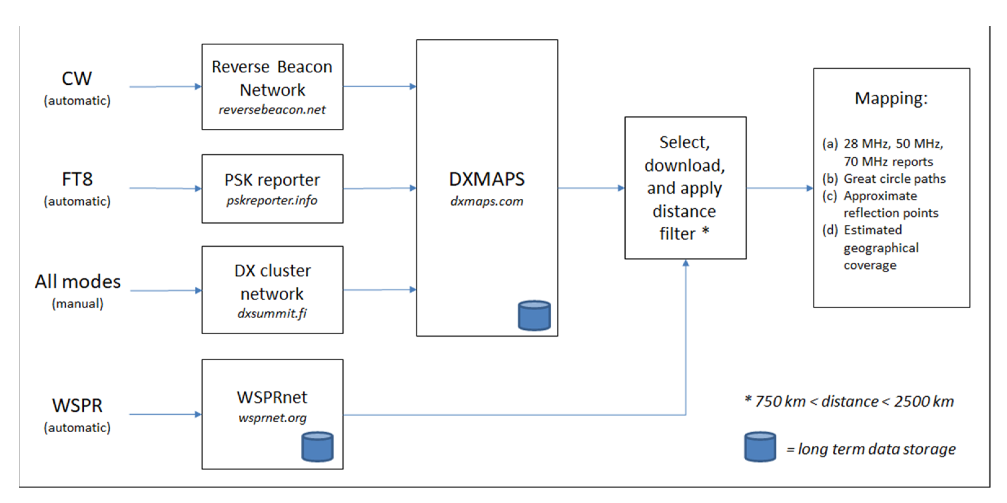
2.1. Es Detection Using Amateur Data

Figure 1 gives an overview of the approach adopted to the collection, filtering, and mapping of amateur radio reception data. Primary sources of data include the Reverse Beacon Network [40], PSK reporter [41], WSPRNet [42], and the DX cluster [43], all of which automatically and continuously collect reports from amateur radio stations of signal reception from other amateur stations. Recorded data include reception date/time, transmitter and receiver locations, and radio frequency, and sometimes also signal strength, doppler shift, and transmitter power. Another system, DXMaps [44], continuously aggregates and archives the data from the primary reporting networks. All these systems are operated on a voluntary basis, but they have proved to be a very reliable information source in recent years.

For this study, selected reception reports were downloaded from DXMaps, supplemented with a subsidiary direct feed from WSPRNet. Reception reports in the 28 MHz, 50 MHz, and 70 MHz amateur frequency bands only were selected, on the basis that at lower frequencies ionospheric propagation modes other than Es are very likely also to be operating, while at higher frequencies Es reflections are relatively rare.

For frequencies in the selected bands, consistent long-distance propagation of signals was much more likely to be via sporadic E than by any other mode. However, to reduce/eliminate possible ground wave, tropospheric, and scatter effects, a minimum station separation of 750 km was applied in the processing.

Similarly, an upper limit of 2500 km was set to reject obvious multi-hop Es paths, so that a single hop could be assumed, allowing a midpoint to be easily assigned to the path to indicate the likely point of reflection.

It was possible that some signals propagated by mechanisms other than Es (particularly meteor scatter) would still be present in the data after distance filtering, but sporadic E has other distinguishing features. Sporadic E reflection is characterized by moderately persistent signals (minutes to hours), and transient, mobile, reflecting clouds of limited horizontal extent (10 km—a few hundred km). Where these characteristics are present, confident identification of Es is possible.

Figure 2 shows an example map of Western Europe, on which are plotted reception reports from a single 15 min period on 18 August 2018. Solid lines indicate the great circle paths between transmitting and receiving stations. It can be seen that there is clear triangulation, from multiple directions, of a number of concentrated areas of reflection.

In order to show the pattern of estimated reflection points more clearly, Figure 3 represents the same reception reports as in Figure 2 but with solid circles indicating the midpoints of the great circle paths, with the paths themselves omitted for clarity.

One of the limitations of using signals of opportunity, such as amateur radio signals, for research is a lack of firm knowledge about which stations were transmitting and/or receiving during the selected time period. Similarly, geographical coverage will inevitably be incomplete where there are no amateur radio stations in suitable locations. Because of these factors, it is clear that, although the presence of a signal path on the map indicates the probable presence of Es, the absence of a signal path in a given location does not reliably indicate the absence of Es.

For these reasons, an estimated coverage plot was derived which shows the midpoints of all possible paths between all stations known (from the reception report data) to have been either transmitting or receiving, on each frequency band, during the selected time period. This is shown by the additional background in Figure 3, in which the estimated geographical coverage is indicated by a small dot for the midpoint of every possible path between active stations.

As an example of the usefulness of the geographical coverage estimate, in Figure 3 it can be seen that the reception reports show no Es reflection points in north-west France, but nonetheless there is a considerable density of coverage markers in that area. This indicates that the apparent local absence of Es was probably genuine.

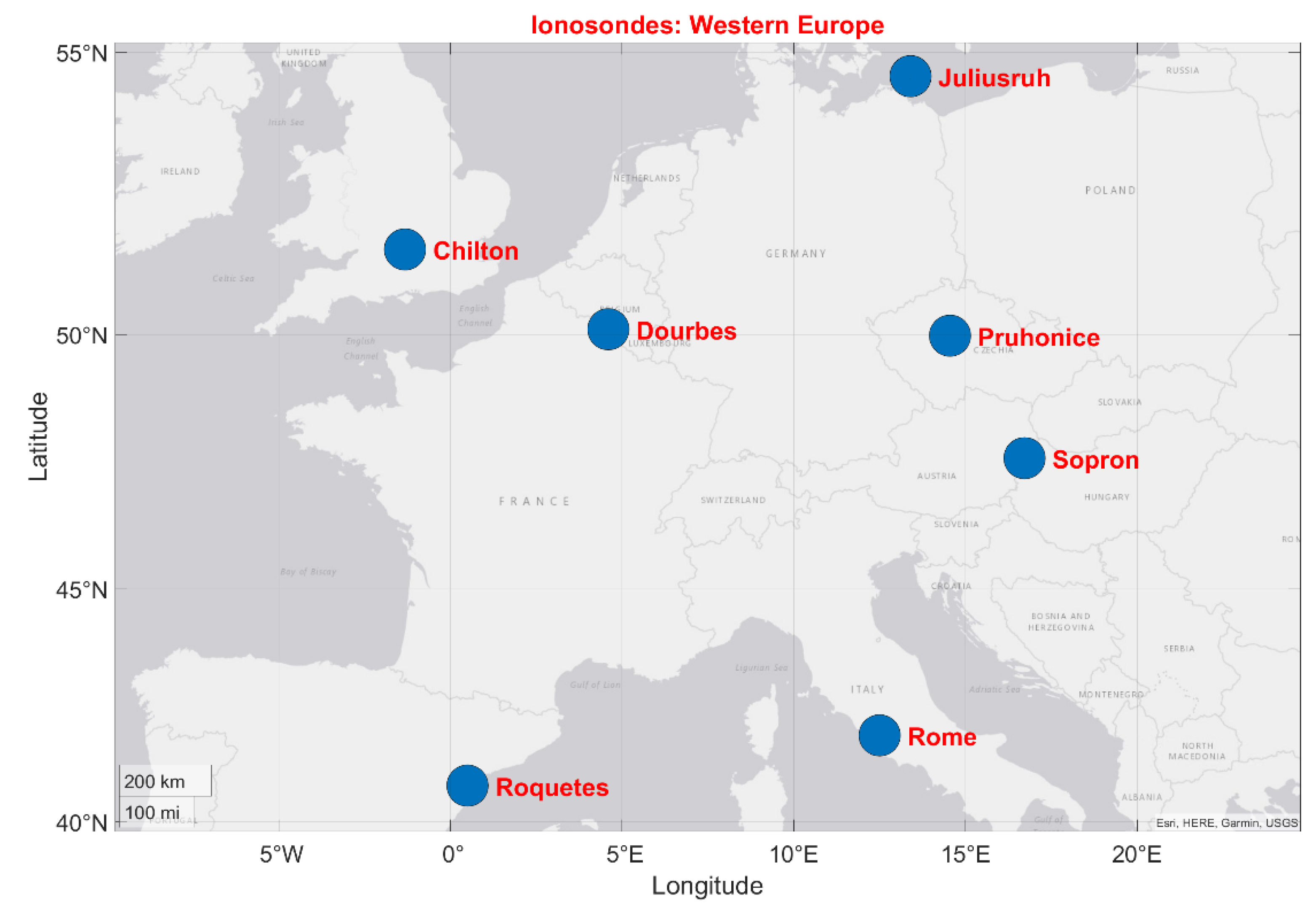
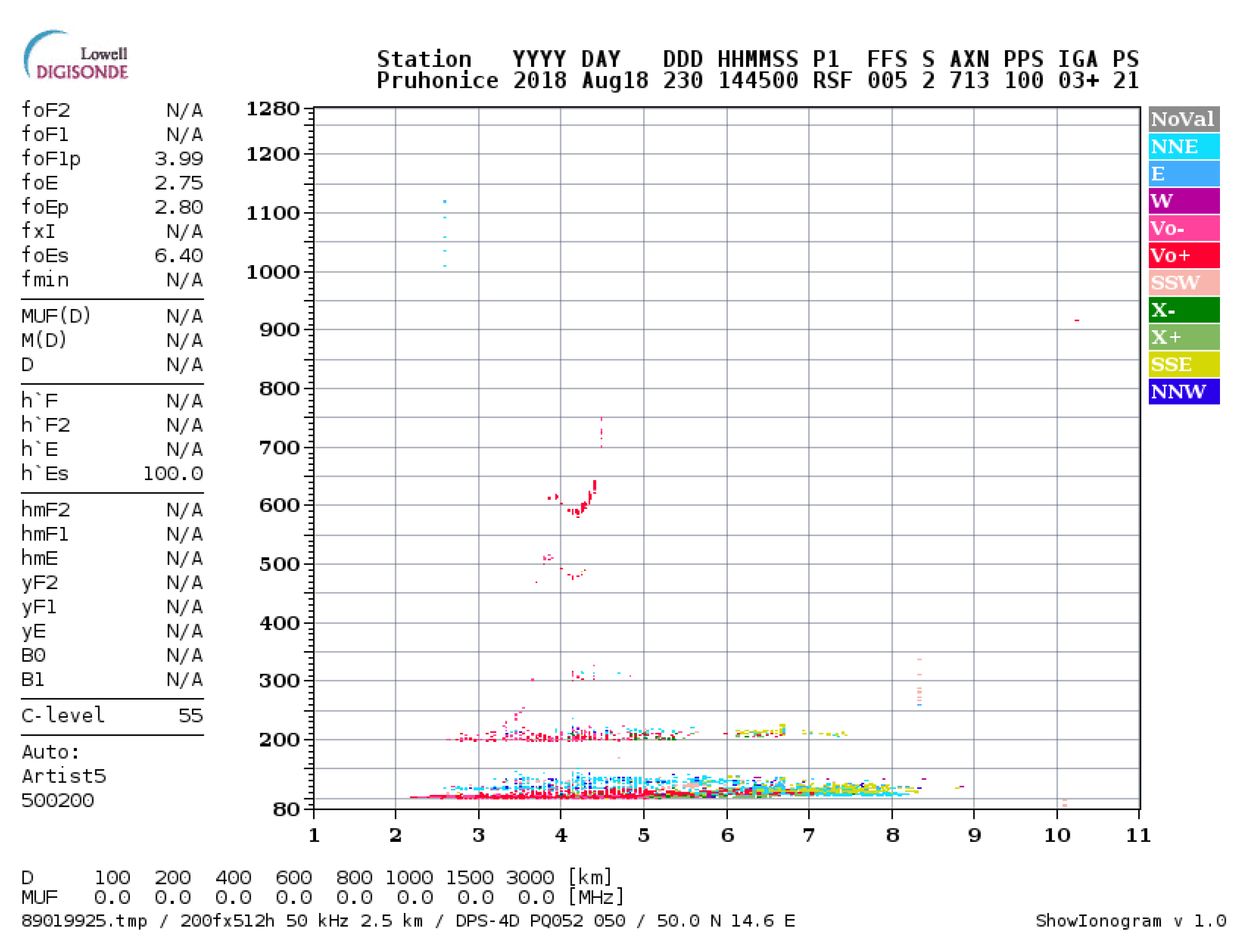
2.2. Validation against Ionosonde Data

Ionosonde data can give unequivocal evidence of the presence or absence of sporadic E. Figure 4 shows a map of the continuously operating ionosondes in the area of this study; the gaps in coverage can clearly be seen, but where Es occurs close to an ionosonde site, valuable information can be gained.

The evidence for sporadic E in ionograms is best found by examination of individual records, although some less rigorous analysis can be performed using auto-scaled observations. Figure 5 shows an example of an ionogram with both F-layer and sporadic E reflections present. They can easily be distinguished by their virtual height, but also because the F-layer traces are strongly curved upwards, due to retardation as the waves are gradually bent back to earth. The sporadic E trace, by contrast, does not curve, because Es layers are very dense and very thin, giving no detectable retardation. In this example, the Es layer is ‘non-blanketing’ (partially transparent), and the reflection from F-layer ionization is clearly visible through it.

By contrast, the example in Figure 6 shows much more intense sporadic E, where the Es peak ionization is well above that in the F region. It also shows evidence of a second Es reflection (shown at 200 km) which is the result of a double bounce from 100 km. F-layer reflections are only just visible through the Es.

For this study, records from seven European ionosondes were individually examined to establish the highest reflection frequency at each observation time. Since we could not distinguish between the ordinary (O) and extraordinary (X) modes from the amateur radio observations, the highest frequency vertically reflected (normally the X but sometimes off-axis) was adopted as the key measure (f_tEs). This approach would not necessarily be valid for lower HF communications, as the X mode often experiences greater absorption, but at 28 MHz and above the difference in absorption between the O and X modes is small.

Each f_tEs value represents a snapshot of the state of the ionosphere in the vicinity of the ionosonde station, at the relevant time stamp.

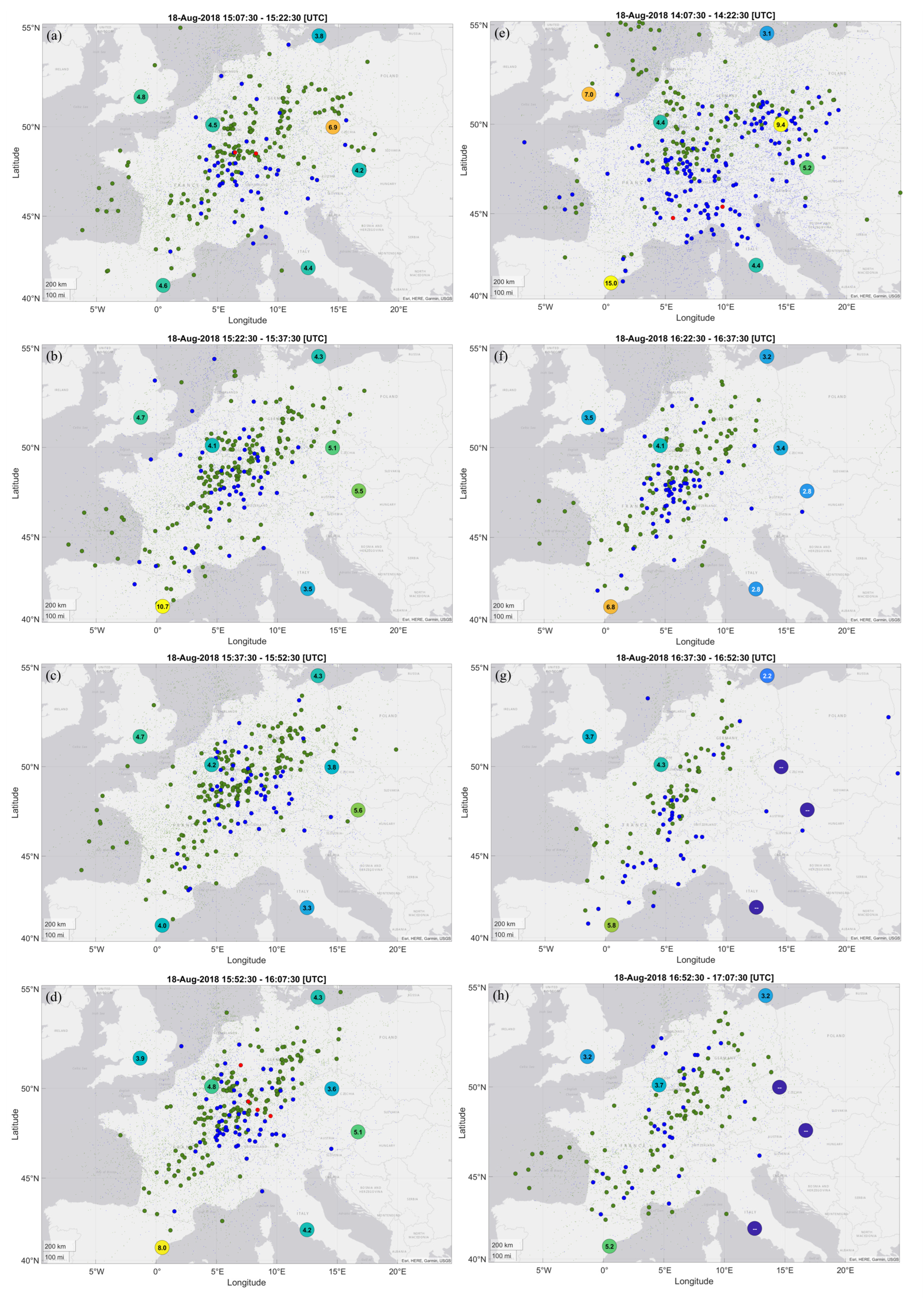
3. Case Study Results

On 18 August 2018, a large-scale sporadic E event developed rapidly over Central and Western Europe in the early afternoon UTC, as shown by Pruhonice ionosonde Es critical frequency data (f_oEs) in Figure 7. F2 critical frequency data (f_oF2) are also shown for comparison. August 2018 was close to solar minimum and the afternoon was unremarkable from an ionospheric index point of view, with a solar flux of 67 and a Kp of 3.

In Figure 8 and Figure 9, the progress of the 18 August 2018 Es event is illustrated with maps showing sequential 15 min periods centered from 13:15 UTC to 15:00 UTC (Figure 8) and 15:15 UTC to 17:00 UTC (Figure 9).

The format of each map is as shown in Figure 3, but with the addition of a large, filled circle at the location of each of the seven ionosondes shown in Figure 4. Each circle includes the corresponding value of f_tEs. Ionosonde color coding, which is provided for guidance only, goes from dark blue (low values) to yellow (high values). Dark blue with two dashes indicates that no Es was detected by the corresponding ionosonde.

Video S1 (see Supplementary Materials) is a video representation of the case study results, also showing mapping of the 18 August 2018 event but with sequential 1 min samples from 13:00 UTC to 17:00 UTC. To aid visual interpretation, all data, including the ionosonde data, are represented with 5 min persistence centered on the relevant time stamp.

4. Case Study Discussion

At 13:15 UTC (Figure 8a), soon after the start of the Es event, a large, intense reflecting area can be seen, centered at about latitude 48 N, longitude 13 E. Local ionosonde data also indicate high values of f_tEs in that region at that time. Over the next hour (Figure 8b–e), another reflecting area gradually developed to the SW, centered at about 46 N 7 E, where there was no local ionosonde for comparison. By 14:00 UTC (Figure 8d), there were two distinct reflecting areas, with a clear gap between them. Good geographical coverage is indicated in that area, so it seems likely that the gap was genuine.

This overall pattern persisted until, from 15:15 UTC (Figure 9a) onwards, the areas of maximum ionization began to merge and to move in a broadly northwesterly direction. Eventually they began to fade, until by 17:00 UTC (Figure 9h) only a relatively weak reflecting area remained, along a NE/SW line, with mainly 28 MHz paths indicated. By this time, three of the eastern-most ionosondes were no longer reporting any Es.

It can be seen that through the whole period, the 28 MHz reflection points (green circles) were generally spread over a wider area than the 50 MHz reflection points (blue circles), and very few 70 MHz reflection points (red circles) are shown at all. This is as expected, given the lower level of level of ionization necessary to support reflection at the lower frequencies.

Across the whole series, good correspondence can be seen between the locations of the concentrations of great circle path midpoints and the nearby ionosonde f_tEs values. Precise and detailed correspondence should not be expected, because the f_tEs figures represent snapshots at the middle of each period, the intense Es clouds are likely to be small, and the derived reflection points can only be approximations because of the possibility of off-axis paths [45]. Nonetheless, the structure and evolution of the event can clearly be seen.

The observed strong clustering of path midpoints, even as the reflecting areas grew, moved, and declined, supports the contention that the vast majority of the signals observed during the case study period were propagated via sporadic E. Meteor scatter would not exhibit these characteristics. In addition, F2 propagation at 28 MHz and above was extremely unlikely at the date of this case study, which was close to sunspot minimum.

5. Conclusions

This article presents a novel observational approach to the study of ionospheric sporadic E, using crowd-sourced radio amateur observations across multiple ground-to-ground links and at multiple radio frequencies.

The temporal and spatial variability of sporadic E is difficult to study because most ionospheric instruments are limited to specific locations and have limited temporal sampling. Examples include ISRs that typically take data in campaign modes at a fixed location, ionosondes that sample every 5–15 min at a few fixed locations, and satellite observations which are sparse both geographically and temporally.

The new technique is demonstrated using a case study of sporadic E over Europe on 18 August 2018. Reception reports from amateur radio stations operating at 28 MHz, 50 MHz, and 70 MHz were used to demonstrate the mapping of sporadic E. For mapping purposes, the midpoint of the transmitter to receiver path was taken as an approximation of the reflection location. The case study clearly illustrates the ability of the technique to reveal the presence and evolution of a sporadic E event: two distinct sporadic E regions were present over Europe for over an hour, subsequently merging and then slowly dispersing. The case study also demonstrates good correspondence with results from seven European ionosondes, as well as clearly demonstrating the presence of Es in the gaps between ionosonde locations.

Compared with traditional techniques, the new approach can provide both better spatial and temporal resolution and wider geographical coverage, particularly in regions of high amateur radio activity such as Europe, North America, and Japan. It can also fill in gaps in the coverage provided by other more sparsely distributed instruments. Amateur radio stations are widely distributed, and many are actively searching for Es events in order to extend their VHF communications.

A limitation of the new technique is that coverage can be missing where there are no amateur radio stations active in suitable locations. Although the presence of a signal path on the map indicates the probable presence of Es, the absence of a reception report in a given location does not reliably indicate the absence of Es. To mitigate this issue, an estimate of geographical coverage is provided per time period.

Improvements to data coverage could be made by strategically placing some additional equipment to cover data gaps. It would also be advantageous to augment the radio amateur equipment with timed signals that could allow inference of additional information such as number of hops.

References

1. Vincent, R.A. The dynamics of the mesosphere and lower thermosphere: A brief review. Prog. Earth Planet. Sci. 2015, 2, 4. [Google Scholar] [CrossRef] [Green Version]
2. Johnson, R.M.; Killeen, T.L. The Upper Mesosphere and Lower Thermosphere: A Review of Experiment and Theory; American Geophysical Union: Washington, DC, USA, 1995. [Google Scholar] [CrossRef]
3. Whitehead, J.D. Recent work on mid-latitude and equatorial sporadic-E. J. Atmos. Terr. Phys. 1989, 51, 401–424. [Google Scholar] [CrossRef]
4. Mathews, J.D. Sporadic E: Current views and recent progress. J. Atmos. Sol. -Terr. Phys. 1998, 60, 413–435. [Google Scholar] [CrossRef]
5. Haldoupis, C. A tutorial review on sporadic E layers. In Aeronomy of the Earth’s Atmosphere and Ionosphere; Abdu, M., Pancheva, D., Eds.; IAGA Special Sopron Book Series; Springer: Dordrecht, The Netherlands, 2011; Volume 2, pp. 381–394. [Google Scholar] [CrossRef]
6. Smith, E.K. Temperate zone sporadic-E maps (foEs > 7 MHz). Radio Sci. 1978, 13, 571–575. [Google Scholar] [CrossRef]
7. Christakis, N.; Haldoupis, C.; Zhou, Q.; Meek, C. Seasonal variability and descent of mid-latitude sporadic E layers at Arecibo. Ann. Geophys. 2009, 27, 923–931. [Google Scholar] [CrossRef] [Green Version]
8. Grebowsky, J.M.; Bilitza, D. Sounding rocket data base of E-and D-region ion composition. Adv. Space Res. 2000, 25, 183–192. [Google Scholar] [CrossRef]
9. Smith, E.K. Worldwide Occurrence of Sporadic E; US Department of Commerce, National Bureau of Standards: Washington, DC, USA, 1957; Volume 582, pp. 178–183. [Google Scholar]
10. Smith, L.G.; Mechtly, E.A. Rocket observations of sporadic-E layers. Radio Sci. 1972, 7, 367–376. [Google Scholar] [CrossRef]
11. From, W.R.; Whitehead, J.D. On the peculiar shape of sporadic-E clouds. J. Atmos. Terr. Phys. 1978, 40, 1025–1028. [Google Scholar] [CrossRef]
12. Kopp, E. On the abundance of metal ions in the lower ionosphere. J. Geophys. Res. Space Phys. 1997, 102, 9667–9674. [Google Scholar] [CrossRef]
13. Mathews, J.D.; Zhou, Q.; Philbrick, C.R.; Morton, Y.T.; Gardner, C.S. Observations of ion and sodium layer coupled processes during AIDA. J. Atmos. Terr. Phys. 1993, 55, 487–498. [Google Scholar] [CrossRef]
14. Yuan, T.; Wang, J.; Cai, X.; Sojka, J.; Rice, D.; Oberheide, J.; Criddle, N. Investigation of the seasonal and local time variations of the high-altitude sporadic Na layer (Nas) formation and the associated midlatitude descending E layer (Es) in lower E region. J. Geophys. Res. Space Phys. 2014, 119, 5985–5999. [Google Scholar] [CrossRef]
15. Cai, X.; Yuan, T.; Eccles, J.V.; Raizada, S. Investigation on the distinct nocturnal secondary sodium layer behavior above 95 km in winter and summer over Logan, UT (41.7° N, 112° W) and Arecibo Observatory, PR (18.3° N, 67° W). J. Geophys. Res. Space Phys. 2019, 124, 9610–9625. [Google Scholar] [CrossRef]
16. Whitehead, J.D. The formation of the sporadic-E layer in the temperate zones. J. Atmos. Terr. Phys. 1961, 20, 49–58. [Google Scholar] [CrossRef]
17. Haldoupis, C.; Pancheva, D.; Singer, W.; Meek, C.; MacDougall, J. An explanation for the seasonal dependence of midlatitude sporadic E layers. J. Geophys. Res. Space Phys. 2007, 112. [Google Scholar] [CrossRef]
18. Qiu, L.; Zuo, X.; Yu, T.; Sun, Y.; Qi, Y. Comparison of global morphologies of vertical ion convergence and sporadic E occurrence rate. Adv. Space Res. 2019, 63, 3606–3611. [Google Scholar] [CrossRef]
19. Yamazaki, Y.; Arras, C.; Andoh, S.; Miyoshi, Y.; Shinagawa, H.; Harding, B.J.; Englert, C.R.; Immel, T.J.; Sobhkhiz-Miandehi, S.; Stolle, C. Examining the wind shear theory of sporadic E with ICON/MIGHTI winds and COSMIC-2 Radio 2 occultation data. Geophys. Res. Lett. 2022, 49, e2021GL096202. [Google Scholar] [CrossRef]
20. Miya, K. My memory of efforts in developing CCIR Recommendation 534-3: Method for calculating sporadic-E field strength. IEEE Antennas Propag. Mag. 1996, 38, 90–93. [Google Scholar] [CrossRef]
21. Smith, E.K.; Igarashi, K. VHF sporadic E—A significant factor for EMI. Proc. Int. Symp. EMC 1997, 29–32. [Google Scholar] [CrossRef]
22. Yue, X.; Schreiner, W.S.; Pedatella, N.M.; Kuo, Y.H. Characterizing GPS radio occultation loss of lock due to ionospheric weather. Space Weather 2016, 14, 285–299. [Google Scholar] [CrossRef] [Green Version]
23. Arras, C.; Wickert, J.; Beyerle, G.; Heise, S.; Schmidt, T.; Jacobi, C. A global climatology of ionospheric irregularities derived from GPS radio occultation. Geophys. Res. Lett. 2008, 35. [Google Scholar] [CrossRef]
24. Arras, C.; Wickert, J. Estimation of ionospheric sporadic E intensities from GPS radio occultation measurements. J. Atmos. Sol. -Terr. Phys. 2018, 171, 60–63. [Google Scholar] [CrossRef]
25. Tsai, L.C.; Su, S.Y.; Liu, C.H.; Schuh, H.; Wickert, J.; Alizadeh, M.M. Global morphology of ionospheric sporadic E layer from the FormoSat-3/COSMIC GPS radio occultation experiment. GPS Solut. 2018, 22, 1–12. [Google Scholar] [CrossRef] [Green Version]
26. Reinisch, B.W.; Galkin, I.A. Global ionospheric radio observatory (GIRO). Earth Planets Space 2011, 63, 377–381. [Google Scholar] [CrossRef] [Green Version]
27. Haldoupis, C.; Meek, C.; Christakis, N.; Pancheva, D.; Bourdillon, A. Ionogram height–time–intensity observations of descending sporadic E layers at mid-latitude. J. Atmos. Sol. -Terr. Phys. 2006, 68, 539–557. [Google Scholar] [CrossRef] [Green Version]
28. Sun, W.; Ning, B.; Yue, X.; Li, G.; Hu, L.; Chang, S.; Lin, J. Strong sporadic E occurrence detected by ground-based GNSS. J. Geophys. Res. Space Phys. 2018, 123, 3050–3062. [Google Scholar] [CrossRef]
29. Baggaley, W.J. Seasonal characteristics of daytime Es occurrence in the southern hemisphere. J. Atmos. Terr. Phys. 1985, 47, 611–614. [Google Scholar] [CrossRef]
30. EBU Technical Centre. Ionospheric propagation in Europe in VHF television band I. In EBU Technical Document TECH 3214; European Broadcasting Union: Brussels, Belgium, 1976. [Google Scholar]
31. Deacon, C.J.; Witvliet, B.A.; Mitchell, C.N. Investigation of the polarization of 50 MHz signals via Sporadic-E reflection. In Proceedings of the Nordic HF Conf (August 2019). Nordic Shortwave Conference, Fårö, Sweden, 12–14 August 2019. [Google Scholar]
32. Deacon, C.J.; Witvliet, B.A.; Steendam, S.N.; Mitchell, C.N. Rapid and accurate measurement of polarization and fading of weak VHF signals obliquely reflected from sporadic-E Layers. IEEE Trans. Antennas Propag. 2020, 69, 4033–4048. [Google Scholar] [CrossRef]
33. Sakai, J.; Saito, S.; Hosokawa, K.; Tomizawa, I. Anomalous propagation of radio waves from distant ILS localizers due to ionospheric sporadic-E. Space Weather 2020, 18, e2020SW002517. [Google Scholar] [CrossRef]
34. Hosokawa, K.; Kimura, K.; Sakai, J.; Saito, S.; Tomizawa, I.; Nishioka, M.; Tsugawa, T.; Ishii, M. Visualizing sporadic E using aeronautical navigation signals at VHF frequencies. J. Space Weather Space Clim. 2021, 11, 6. [Google Scholar] [CrossRef]
35. Miya, K.; Shimizu, K.; Kojima, T. Oblique-incidence sporadic-E propagation and its ionospheric attenuation. Radio Sci. 1978, 13, 559–570. [Google Scholar] [CrossRef]
36. Frissell, N.A.; Miller, E.S.; Kaeppler, S.R.; Ceglia, F.; Pascoe, D.; Sinanis, N.; Smith, P.; Williams, R.; Shovkoplyas, A. Ionospheric sounding using real-time amateur radio reporting networks. Space Weather 2014, 12, 651–656. [Google Scholar] [CrossRef]
37. Frissell, N.A.; Katz, J.D.; Gunning, S.W.; Vega, J.S.; Gerrard, A.J.; Earle, G.D.; Moses, M.L.; West, M.L.; Huba, J.D.; Erickson, P.J.; et al. Modeling amateur radio soundings of the ionospheric response to the 2017 Great American Eclipse. Geophys. Res. Lett. 2018, 45, 4665–4674. [Google Scholar] [CrossRef]
38. Frissell, N.A.; Vega, J.S.; Markowitz, E.; Gerrard, A.J.; Engelke, W.D.; Erickson, P.J.; Miller, E.S.; Luetzelschwab, R.C.; Bortnik, J. High-frequency communications response to solar activity in September 2017 as observed by amateur radio networks. Space Weather 2019, 17, 118–132. [Google Scholar] [CrossRef] [Green Version]
39. Frissell, N.A.; Kaeppler, S.R.; Sanchez, D.F.; Perry, G.W.; Engelke, W.D.; Erickson, P.J.; Coster, A.J.; Ruohoniemi, J.M.; Baker, J.B.; West, M.L. First Observations of Large Scale Traveling Ionospheric Disturbances Using Automated Amateur Radio Receiving Networks. Geophys. Res. Lett. 2022, 49, e2022GL097879. [Google Scholar] [CrossRef]
40. Available online: http://reversebeacon.net/ (accessed on 20 December 2021).
41. Available online: https://pskreporter.info/ (accessed on 20 December 2021).
42. Available online: https://www.wsprnet.org/ (accessed on 20 December 2021).
43. Available online: http://www.dxsummit.fi/ (accessed on 20 December 2021).
44. Available online: https://www.dxmaps.com/ (accessed on 20 December 2021).
45. Miya, K.; Sasaki, T. Characteristics of ionospheric Es propagation and calculation of Es signal strength. Radio Sci. 1966, 1, 99–108. [Google Scholar] [CrossRef]
46. Deacon, C.J. Data and code for “Consolidated Amateur Radio Signal Reports as Indicators of Intense Sporadic E Layers”. Bath Univ. Bath Res. Data Arch. 2022. [Google Scholar] [CrossRef]
Figure 1. Overview of the approach to the collection, filtering, and mapping of amateur radio reception reports. * The distance filter selects for path lengths between 750 km and 2500 km (see text).
Atmosphere 13 00906 g001
Figure 2. Example map showing reception reports from a 15 min period centered on 14:45 UTC 18 August 2018. Solid lines indicate the great circle paths between the transmitting and receiving stations. Green = 28 MHz, blue = 50 MHz, red = 70 MHz.
Atmosphere 13 00906 g002
Figure 3. Example map showing the midpoints of reported signal paths from the same period as in Figure 2, plus the estimated geographical coverage of the data. Solid circles represent the midpoints of reported great circle paths. Background dots indicate the estimated geographical coverage (see text). Green = 28 MHz, blue = 50 MHz, red = 70 MHz.
Atmosphere 13 00906 g003
Figure 4. Continuously active ionosondes in Central and Western Europe.
Atmosphere 13 00906 g004
Figure 5. Pruhonice ionosonde plot 18 August 2018, 15:45 UTC. F-layer reflection (curved traces) can be seen above 200 km virtual height. E-layer reflection (horizontal trace) can be seen at just over 100 km virtual height.
Atmosphere 13 00906 g005
Figure 6. Pruhonice ionosonde plot 18 August 2018, 14:45 UTC. Intense Es reflections (horizontal trace) can be seen at around 100 km virtual height, with a second bounce (via ground) at 200 km.
Atmosphere 13 00906 g006
Figure 7. Autoscaled foF2 (red) and foEs (blue) from the Pruhonice ionosonde for 18 August 2018.
Atmosphere 13 00906 g007
Figure 8. (ah). First part of sporadic E event 18 August 2018, sequential 15 min samples centered from 13:15 UTC to 15:00 UTC. Large circles: ionosonde-derived ftEs [MHz] (dark = low, pale = high, -- = no Es). Medium circles: approximate signal reflection points (green = 28 MHz, blue = 50 MHz, red = 70 MHz). Dots: estimated coverage (colors ditto).
Atmosphere 13 00906 g008
Figure 9. (ah). Second part of sporadic E event 18 August 2018, sequential 15 min samples centered from 15:15 UTC to 17:00 UTC. Large circles: ionosonde-derived ftEs [MHz] (dark = low, pale = high, -- = no Es). Medium circles: approximate signal reflection points (green = 28 MHz, blue = 50 MHz, red = 70 MHz). Dots: estimated coverage (colors ditto).
Atmosphere 13 00906 g009
Publisher’s Note: MDPI stays neutral with regard to jurisdictional claims in published maps and institutional affiliations.