Article

Comparison of Cloud Amounts Retrieved with Three Automatic Methods and Visual Observations

by
María Pilar Utrillas
1,
María José Marín
2,*,
Víctor Estellés
1,3,
Carlos Marcos
1,
María Dolores Freile
1,
José Luis Gómez-Amo
1 and
José Antonio Martínez-Lozano
1
1
Solar Radiation Group, Departament de Física de la Terra i Termodinàmica, Universitat de València, 46100 Burjassot, Spain
2
Solar Radiation Group, Departament de Matemàtiques per a l’Economia i l’Empresa, Universitat de València, 46022 Valencia, Spain
3
Consiglio Nazionale delle Ricerche, Istituto Scienze dell’Atmosfera e del Clima, 00133 Roma, Italy
*
Author to whom correspondence should be addressed.
Atmosphere 2022, 13(6), 937; https://doi.org/10.3390/atmos13060937
Submission received: 3 May 2022 / Revised: 25 May 2022 / Accepted: 26 May 2022 / Published: 9 June 2022
(This article belongs to the Section Atmospheric Techniques, Instruments, and Modeling)

Abstract

:
Four methods have been used for the estimation of the total cloud amount and cloud amount for low clouds: visual observations, the Long method applied on pyranometer measurements, the Automatic Partial Cloud Amount Detection Algorithm (APCADA) method applied on pyrgeometers measurements, and ceilometer measurements of the cloud base height. Records from meteorological observers indicate that clear days (0–1 octa) represent the most frequent cloud amount for low clouds. In contrast, the total cloud amount is more aleatory. Results obtained from the Long method show maximum frequency in the extreme cloud amount values. The APCADA method also indicates the predominance of cloudless skies. The ceilometer method shows a predominance of completely clear skies, but the completely cloudy (8 octas) is the second most frequent case. Automatic methods report more cloudless and overcast skies than the observer. Automatic methods agree with the visual method or differ in ±1 octa for 60–76% cases for low cloud amount and for 56–63% cases for total cloud amount. In general, low cloud amount agrees more with observer measurements than total cloud amount and the automatic methods underestimated total cloud amount observer values possibly due to the difficulty in monitoring high clouds.

1. Introduction

Clouds are the most critical factor in modulating the terrestrial radiative balance and determining climate sensitivity [1]. They reflect solar radiation to space, absorb and re-emit the longwave radiation emitted by the Earth surface and the low troposphere [2,3,4], and they must be considered in numerical models.
Clouds present the highest uncertainties for estimating and interpretating of the changing Earth radiation balance [5]. These uncertainties are caused by the scarceness of surface based global measurements, inhomogeneity in the existent datasets, and low precision in the measurement of small changes in cloudiness that scale to a significant impact on the terrestrial climate [6,7].
A particular case of interest is the estimation of cloud amount. It represents the fraction of the sky covered by clouds of a particular type or combination. Since clouds are the largest attenuating factors of solar radiation, cloud cover is a useful predictor of solar resource [8] and photovoltaic solar energy [9]. Experimental determination of the cloud amount can be performed using remote sensing techniques based on satellite platforms [10,11,12], or surface-based [13]. Ground-based remote sensing methods could be hemispheric or column techniques. Shortwave or longwave radiation from the sky is used to retrieve the cloud amount, e.g., using pyranometers or pyrgeometers in the former and a vertical portion of the sky to retrieve the nadir projected cloud fraction and later the cloud amount using ceilometers in the latter. Moreover, some instruments can continuously obtain the cloud amount during the day and at night, such as pyrgeometers, while others can only be used during the day, such as the total sky imager. Tapakis and Charalambides [14] presented a quite complete review of the equipment and methodologies for cloud detection and classification. Unfortunately, the temporal evolution of cloud amount on decadal and longer scales is unclear, mainly because of uncertainties in both satellite [15,16] and surface-based observational records [17].
For quite a long time now, the determination of the cloud amount has been simply performed by visual observation (i.e., subjective) from surface level [18,19,20]. Three times a day, meteorological observers routinely record total cloud amount, cloud amount at low levels and type of clouds [18]. This method is inherently subjective, and it can be conditioned by factors, such as the extension of the sky view and the uneven illumination of the cloud deck at night from the surface [21,22]. Further, the cloud amount errors increase for low elevation angles because the human observer cannot identify the spaces between clouds but the cloud wall itself, overestimating the apparent cloud amount [23].
Despite its obvious utility, the meteorological observations are associated to a lack of homogeneity in the methodology and observation times. The method is rudimentary (limited to octas of the sky dome) and performed by a subjective human being, therefore making the method less reliable. Nowadays, the reduction of costs has pushed for the implementation of more automatic methods with a reduced human role [13]. The instruments and algorithms devised for cloud identification and discrimination of clear/cloud boundaries improved largely, reducing the cloud amount and distribution determination uncertainties [24]. The development of automatic detection systems is now priority as visual observations must be substituted by automatic measurements [3,25,26]. For instance, differences in cloud characteristics introduced by the automation at the Royal Netherlands Meteorological Institute (KNMI) are described by Wauben [27] and Wauben et al. [28]. This transition resulted in discontinuities in time series of cloud observations that cannot be rectified posteriori.
This study’s first automatic cloud detection method is based on shortwave downward radiation measurements performed by pyranometers. Long et al. [29] estimated the cloud fraction using high resolution measurements of global and diffuse solar radiation, based on the methodology previously proposed by Long and Ackerman [30] for the separation of clear and cloudy skies. Besides, Durr and Philipona [31] developed the Automatic Partial Cloud Amount Detection Algorithm (APCADA) for estimating the cloud amount directly from measurements of longwave downward radiation measured by pyrgeometers.
One of the most prominent instruments available for the determination of cloud amount is the ceilometer. The ceilometer is a specific type of LiDAR (light detection and ranging), based on the principle of elastic backscattering: it emits light pulses vertically into the atmosphere and measure the light backscattered by clouds at different altitudes [13,32,33]. These observations can be used to calculate the cloud amount by averaging the binary cloud state over a particular period of time.
In our study, we compared the cloud amounts determined with the three automatic methods with the values recorded from a meteorological observer for the five years 2013–2017. For example, a few studies have already compared pairs of the three methods [13]. However, to our best knowledge, no previous study has dealt with a comparison of the three automatic methods proposed in this article. We have not included satellite-based data, although the reader can find such studies, e.g., by Ackerman et al. [34]; Werkmeister et al. [35]; An and Wang [36]; Calbó et al. [37]. The ultimate objective has been to find quantitative relationships between the automatic and visual cloud amount estimations. These relationships would help to understand how to continue the meteorological series of visual observations, already discontinued in many observatories worldwide.
This article has been organized as follows: Section 2 describes the experimental setup and the methodology used. The results are presented in Section 3. Main conclusions have been summarized in Section 4.

2. Materials and Methods

This study takes as a reference the cloud amount values registered by a meteorological observer at the airport of Manises (Valencia), located 5 km SW from the Burjassot campus, at the synoptic hours 7, 13, and 18. These cloud amount observations were recorded by the State Agency of Meteorology (AEMET). The records are coded as an integer number between 0 and 8. The value of 0 octa corresponds to clear skies (0% cloud fraction) and 8 octa to overcast skies (100% cloud fraction). According to the guidelines of the WMO [21], a single cloud in a clear sky should be registered as 1 octa, while a tiny gap in an overcast sky is registered as 7 octa. This means that 1 and 7 octa represent a larger range of fractional cloudiness conditions (18.75%) than from 2 to 6 octa (12.5%). Table 1 shows the conversion of the cloud fraction expressed in percentage to octa [13].
The automatic measurements were recorded on the roof of the Faculty of Physics, located on the Burjassot campus of the University of Valencia (39°30′ N; 0°25′ W; 60 m a.s.l). The automatic instruments used to determine the cloud amount were: a pyranometer, a pyrgeometer, and a ceilometer. All methods used in this work calculate the cloud amount in percentages, except for APCADA that provides it in octa. The transformation of the cloud amount from percentages to octas was done by assuming the conversion from Table 1. Although the sites where the meteorological observer and the automatic methods operate are different, we assume that the sky condition is the same, given that the distance is shorter than 5 km, and the vertical difference is only 18 m (i.e., the area in which both sites are located, is flat).
The specific instrumentation and the method used for the estimation of the cloud amount are described below:

2.1. Pyranometer (Long et al. 2016 Method)

The downwelling solar radiation measurements were registered with two Kipp-Zonen CMP21 pyranometers mounted on a Kipp-Zonen Solys-2 sun-tracker, equipped with GPS antenna and active solar tracker. One of them measures the global hemispherical downward radiation, and the other uses a shadow ball to measure the diffuse component. The CMP21 is a secondary standard which measures shortwave solar radiation in the spectral range from 285 to 2800 nm. The temperature of the pyranometer is monitored with a Pt-100 thermal sensor. The temperature dependence of the sensitivity is 0.5%. Its cosine response is 1% for solar zenith angles up to 80° according to the manufacturer’s specifications [38]. Both pyranometers are also installed on two CVF1 ventilation units to minimize occasional dew built up on the domes and reduce thermal offset. Pyranometer measurements are performed every 5 s and the average is registered every 1 min.
The cloud amount is determined by the method of Long et al. [29]. The first step in this method is to identify the clear-sky periods for a 160° field of view, using only 1-min measurements of the downwelling total and diffuse shortwave irradiance [30]. Then, the dataset is screened for overcast and clear-sky cases, and afterwards the cloud amount is estimated for the remaining data. The fractional sky cover is estimated using the normalized diffuse cloud effect, which includes both the measured and clear fit diffuse irradiances, and the clear fit total shortwave irradiance. These values are all tailored to the characteristics of each instrument system. The cloud amount obtained by this methodology shows a high degree of repeatability for well-maintained radiometers [29].

2.2. Pyrgeometer (APCADA Method)

Downwelling longwave radiation measurements were taken with a Kipp & Zonen CGR4 pyrgeometer, mounted on the same Kipp & Zonen Solys-2 sun-tracker and equipped with a second shadow ball. The CGR4 pyrgeometer uses a dome that provides a 180° field of view with negligible directional response error. This instrument was calibrated in 2011 at the WMO premises in Davos, and subsequently calibrated by intercomparison in two measurement campaigns in 2013 and 2015 in Lampedusa, Italy. On all these occasions, the pyrgeometer showed absolute stability, with differences between the calibration coefficients less than 1%.
Dürr and Philipona [31] developed the Automatic Partial Cloud Amount Detection Algorithm (APCADA) for estimating the cloud amount without high clouds directly from longwave downward radiation (LDR), air temperature, and humidity.
The determination of partial cloud amount according to APCADA is based on two parameters: the cloud-free index (CFI) and the variability of longwave downward radiation (STD LDR). The CFI is calculated as:
CFI = LDR AC σ T L 4
where σ is the Stefan–Boltzmann constant, TL the air temperature in Kelvin, ϵAC the emissivity of a cloud-free sky.
Usually, clear skies are represented by CFI ≤ 1, whereas CFI > 1 result in cloudy skies, so this parameter is used to distinguish between clear or cloudy conditions. Furthermore, variability of the longwave downward radiation during the previous 60 min is calculated, as it allows the distinction between cloud fraction types: broken clouds strongly influence the variability signal, while overcast and cloudless skies lead to a low variability. This way, cloud amount is obtained combining the information given by the CFI and the longwave radiation variability, according to the intervals defined by Durr and Philipona [31]. As a drawback, APCADA is able to detect only those clouds that have a measurable effect on longwave downward radiation. Hence, the APCADA algorithm has a limited sensitivity for high (i.e., cold) clouds.

2.3. Ceilometer

The ceilometer used in this work is a CL51 system from Vaisala. The CL51 uses a diode laser that emits short light pulses (~110 ns) to the atmosphere at 910 nm with a repetition rate of 6.5 kHz. The light backscattered by the atmosphere constituents between 0 and 15 km altitude is detected by the system with a vertical resolution of 10 m. The CL51 deployed at the Burjassot station measures the backscattered light with an off-nadir angle of 12° and it is configured to retrieve vertical profiles of the atmosphere every minute. The system’s software is equipped with the Sky Condition Algorithm provided by Vaisala [39]. This algorithm uses measurements from the last 30 min to estimate the cloud cover fraction (CCF) at different altitudes. The altitudes corresponding to the CCF estimations are not fixed and depend on the spatial distribution of clouds in the atmosphere. Total cloud cover, C, of an altitude interval limited by h0 and hf, is estimated by Equation (2):
C = max ( CCF h ) + ( 1 max ( CCF h ) ) h 0 h f max ( CCF h )
where max (CCFh) is the maximum cloud cover value at height h. Equation (2) is used for four different height intervals (0–3 km), (0–7 km), (0–10 km), and (0–15 km). Layers 0–3 and 0–15 km can represent low clouds and total cloud amount respectively.
The CL51 ceilometer method provides cloud amount data every minute, 24 h a day. Nevertheless, for the purposes of this study, only cloud amount obtained during day time has been considered.
Table 2 summarizes the characteristics of the previous methods as well as the number of registered data in the study and the number of simultaneous data with the automatic methods and the meteorological observer.

3. Results

3.1. Analysis of the Cloud Amount Obtained by the Different Methods

The cloud amount has been obtained by a meteorological observer and with the three automatic methods. The first one was estimated with the pyranometers by applying the Long method. The second automatic method analysed was the APCADA method applied on the pyrgeometer data. In the case of the ceilometer, the maximum altitude sensed is 15 km. We have calculated the cloud amount at four different altitude intervals: 0–3 km, 0–7 km, 0–10 km, and 0–15 km (the last one is expected to be more representative of the total cloud amount).
Figure 1 represents the frequency of the low cloud amount values estimated by a meteorological observer considered all together for the three synoptic hours, low-medium cloud amount by APCADA, low cloud amount for ceilometer (0–3 km), and low-medium cloud amount for ceilometer (0–7 km).
Most of the observations (approximately 67%) correspond to clear skies (i.e., between 0 and 1 octa) for low clouds by observer. The APCADA method also found a decreasing frequency with the number of octas: it is maximum, about 23–28%, for 0 and 1 octa, respectively, and decreases to around 5% for the intermediate cloud amounts. Very cloudy skies are also more frequent than intermediate cases, with a frequency of 9% and 7% for 7 and 8 octas respectively. The maximum frequency with the ceilometer appears at 0 octas (completely clear) for both the intervals, with a frequency higher than 69% for clouds in the lowest interval (0–3 km). The second most frequent cloud amount is 8 octas (overcast) with a frequency of 16% (0–7 km). Any of the intermediate amount values are less frequent. It is apparent that the cloud ceilometer overestimates 0 and 8 octa occurrences and it underestimates intermediate cloud coverages in agreement with other authors results [8].
Figure 2 represents the frequency of total cloud amount values estimated by a meteorological observer considered altogether for the three synoptic hours, following the Long method and by the ceilometer (0–10 km and 0–15 km).
In contrast with low cloud observations, the frequency of the meteorologist total cloud amount is more homogeneously spread, with no clear dominance for any given number of octas. Regarding the Long results, the frequency strongly decreases with the number of octas, with the absolute maximum found for 1 octa (~26%) and minimum for 7 octas (~4%). However, the method estimates that the 8 octas case (overcast) is also well represented (~22%).
Regarding ceilometer results, Figure 1 and Figure 2 also indicate that when the considered layer top gradually increases (3 km to 15 km), the frequencies for non-clear skies cases increase at the expense of the frequency for the completely clear case. For example, for measurements up to 3 km, about a 69% of the cases correspond to 0 octas and 10% approximately correspond to 8 octas. If the 0–15 km interval is considered, then 36% of the cases correspond to 0 octas and 26% to 8 octas. This means that considering the 0–3 km layer, the completely clear cases increase by 33% in terms of frequency, and the overcast skies decrease in frequency by 16%, in comparison to the 0–15 km layer. Intermediate layers offer intermediate results: extending the upper limit implies that more clouds will be included in the estimation of the cloud amount. These results agree with Wagner and Kleiss. They used a ceilometer (CEIL) (with cloud-base height up to 3660 m) and a micropulse lidar (MPL) (with cloud-base height up to 20 km); see Figure 2 in [40].
To sum up, automatic methods report more cloudless (0–1 octa) and overcast skies (8 octas) than the observer and it agrees with the results of Boers et al. [13]. Only the APCADA method reports less cloudless (51%) than the observer for low clouds (67%).
We have calculated the annual statistics for cloud amount expressed in octas. The mean cloud amount for low clouds is 1.6 (observer and ceilometer 0–3 km) and for low-medium clouds is 2.7 (APCADA and ceilometer 0–7 km). Layer 0–3 km considers low clouds only. However, layer 0–7 km considers low and medium cloudiness as the APCADA method does (see Table 2). For this reason, the mean value by observer agrees with ceilometer 0–3 km and APCADA method agrees with ceilometer (0–7 km). The medians are 1 (observer and APCADA) and 0 (ceilometer 0–3 km and 0–7 km) with standard deviations 2, 2.7, 2.8, and 3.3 respectively, which represents a similarly high deviation by APCADA and ceilometer methods and higher than the observer method.
The mean cloud amount for total cloudiness is 3.5, 2.9, 3.1, and 3.4 for the observer, Long method, ceilometer (0–10 km), and ceilometer (0–15 km), respectively. The medians are 3 octas for observer, 1.4 octas for Long method and ceilometer 0–10 km, and 2 octas for ceilometer 0–15 km, with standard deviations between 2.5 and 3.4, which is a very high deviation due to the great variety of values that exist. Again, automatic methods have higher standard deviations than the observer method.

3.2. Comparison between Automatic and Visual Methods

In order to evaluate the performance of the automatic methods as a mean for the continuation of the meteorological series of visual observations, we first need to compare the series for the period analysed in this study.
Figure 3 represents the frequency distribution of absolute differences between the simultaneous low or low-medium cloud amount obtained with the observer and the two automatic methods (APCADA and ceilometer 0–3 and 0–7 km). The frequency is expressed in percentage and the cloud amount differences are expressed in octas. The two automatic methods agree or differ in one octa with the human observer among 60% (ceilometer, 0–7 km), 69% (APCADA), and 76% (ceilometer, 0–3 km). Besides, zero octas is the most frequent value. If an octa is considered the measurement uncertainty, the results can be appropriate to reproduce the visual observations with automatic methods. In the two methods we found an overestimation of the low cloud amount, i.e., there are more negative differences except for the ceilometer in the 0–3 km layer.
Suppose we calculate the coincidences defined by cases with a cloud amount difference within ±1 octa, for different ceilometer layers whose upper limit is varied between 2 and 15 km at steps of 1 km. In that case, the layer that gives the maximum number of coincidences is 0–3 km [41]. To some extent, we could consider that this would be the effective altitude of the low clouds registered by the observer, instead of the expected 0–2 km.
The frequency distributions of total cloud amount differences are presented in Figure 4. The maximum number of coincidences or discrepancies in one octa (63%) happens for the ceilometer, layer 0–15 km (56% for the Long method). The percentages are worse than for low clouds (Figure 3), probably due to the difficulty in detecting high clouds. In the two cases, the automatic methods derived cloud amount values are underestimated due to the different measurement principle adopted by these instruments. It is not possible to find a complete agreement between observations and any automatic method [13]. Regarding the APCADA method, results agree with Schade et al. [42], who found a 60% ± 1 octa for all clouds and 73% ± 1 octa at no cirrus conditions.

3.3. Relationships between Automatic and Visual Methods

Once we have analysed the absolute differences between the different automatic and visual methods, it is interesting to derive numerical relationships that allow us to estimate corrected values of cloud amount that are more consistent with the reference series registered by the meteorological observer. For simplicity, linear regressions have been performed only, as shown in Table 3 (low-medium cloud amount) and Table 4 (total cloud amount).
Instead of using instantaneous data as in the previous sections, for the establishment of the relationships, we first calculated the average of the cloud amount values given by each of the automatic methods, for a given cloud amount registered by the observer. This way, for each automatic method, we get nine data points corresponding to 0, 1, …, 8 octas registered by the observer. The relationships have been obtained separately for seasons.
The ceilometer (0–3 km) correlates better than the other two methods (APCADA and ceilometer (0–7 km) with a slope near 1, as shown in Table 3, because until 3 km high only low cloud amount is detected. It is possible that the observer method does not detect medium clouds as the APCADA and ceilometer (0–7 km) do.
A good agreement between the observer method and the two automatic methods is shown for total cloud amount, per Table 4, even better than for low-medium cloud amount, shown in Table 3. There is not any significant change in formulae with season and the correlation coefficient is always higher than 0.94.

4. Conclusions

In this study, we have performed an analysis of three different automatic methods for the estimation of cloud amount at low levels and total cloud amount: The Long method applied to pyranometer measurements, the APCADA method applied to longwave measurements of a pyrgeometer, and the analysis of ceilometer profiles at several atmospheric layer depths. The results from the three automatic methods have been compared to visual estimations of a meteorological observer to understand the similarity between automatic and visual methods. After binning the datasets, we found linear relationships between the automatic and visual methods for different altitudes, namely for low cloud amount and total cloud amount, and different atmospheric profile depths. The relationships proposed here could be used to compare the automatic methods with the observations, but a specific algorithm would be necessary, with data from various instruments (hemispheric and column techniques and more information, such as the altitude of the cloud base) to be able to complete the cloud amount when the observer series is discontinued [13].
In particular, the results can be summarized as follows:
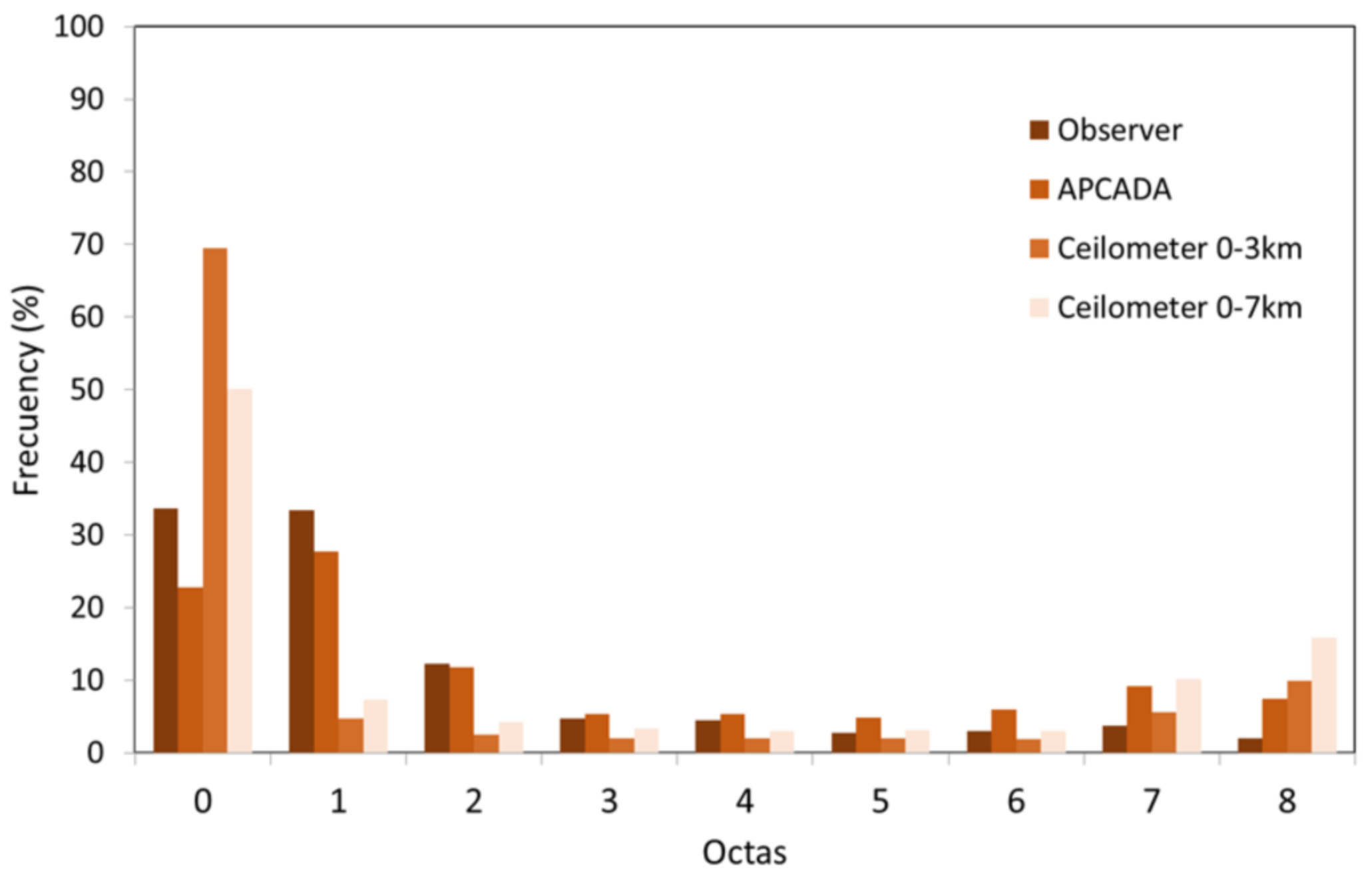
  • Visual observations of the low cloud amount indicate that most of the time (approximately 67% of the records) the sky can be considered clear (cloud amount between 0 and 1 octa). In contrast, the total cloud amount is more variable, with no evident dominance of any cloud cover class.
  • The application of the APCADA method on the pyrgeometer data also show that clear skies are dominant (0–1 octas). The remaining cloud amount values are registered with a 5–12% frequency.
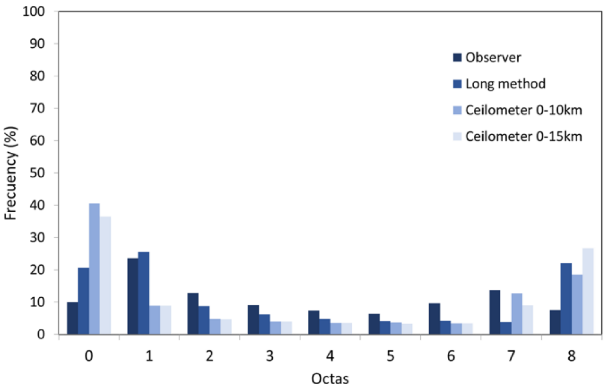
  • The application of the Long method on the pyranometer measurements shows that the frequency, in relation to the number of octas, is higher for the extreme cloud amount values (0–1 and 8 octas). The remaining cloud amounts are more uniformly represented with percentages between 4% and 9%.
  • The ceilometer results are also consistent with the other two automatic methods, because the clear skies are also dominant. In particular, the maximum frequency corresponds to completely clear skies, with a frequency of 69% for low clouds (0–3 km). Overcast skies are also frequent (8 octas), specially for the 0–15 km layer, with a frequency of almost 26%. Any of the remaining values of cloud amount are less frequent than the extremes.
  • The mean cloud amount ranges between 1.6 to 2.7 octas for low-medium clouds and 2.9 to 3.5 octas for total cloud amount. Standard deviation ranges between 2 to 2.8 for low clouds and 2.5 to 3.4 for total cloud amount.
To sum up, automatic methods report more cloudless (0–1 octas) and overcast (8 octas) skies than the observer, except the APCADA method for cloudless skies and low clouds.
If we consider one octa as the measurement uncertainty, automatic methods can reproduce the observer results, especially the ceilometer (0–3 km) and APCADA for partial low cloud amount. These methods agree or differ in one octa in 76% and 69% respectively. Concerning the total cloud amount, the ceilometer (0–15 km) shows a better result (63%) than the Long method (56%). In general, low cloud amount agrees more with observer measurements than total cloud amount and the automatic methods underestimated total cloud amount observer values, possibly due to the difficulty in monitoring high clouds.
We have also compared the results from the automatic methods with the estimations from the visual method and performed linear fittings to relate each of the automatic methods with the reference observer method. Significant changes were not detected with season.

Author Contributions

Conceptualization, M.P.U. and J.A.M.-L.; methodology, M.J.M. and V.E.; validation, V.E., C.M., M.D.F. and J.L.G.-A.; formal analysis and investigation, C.M., M.D.F. and J.L.G.-A.; data curation, M.P.U. and V.E.; writing—original draft preparation, J.A.M.-L.; writing—review and editing, M.J.M. and M.P.U.; visualization and supervision, M.J.M.; project administration, M.P.U.; funding acquisition, M.P.U. and J.A.M.-L. All authors have read and agreed to the published version of the manuscript.

Funding

This work was financed jointly by the Spanish Ministry of Economy and Competitiveness (MINECO) and the European Regional Development Fund (FEDER) through projects CGL2017-86966-R and RTI2018-096548-B-I00 and by the Valencia Autonomous Government through project AICO/2021/341.

Institutional Review Board Statement

Not applicable.

Informed Consent Statement

Not applicable.

Data Availability Statement

Not applicable.

Acknowledgments

We acknowledge the staff from the Spanish State Agency of Meteorology (AEMET) for the cloud amount data recorded at the Manises airport (Valencia).

Conflicts of Interest

The funders had no role in the design of the study; in the collection, analyses, or interpretation of data; in the writing of the manuscript, or in the decision to publish the results.

References

  1. Free, M.; Sun, B.; Yoo, H.L. Comparison between Total Cloud Cover in Four Reanalysis Products and Cloud Measured by Visual Observations at U.S. Weather Stations. J. Clim. 2016, 29, 2015–2021. [Google Scholar] [CrossRef]
  2. Mitchell, D.I.; Finnegan, W. Modification of cirrus clouds to reduce global warming. Environ. Res. Lett. 2009, 4, 045102. [Google Scholar] [CrossRef]
  3. Kazantzidis, A.; Tzoumanikas, P.; Bais, A.F.; Fotopoulos, S.; Economou, G. Cloud detection and classification with the use of whole-sky ground-based images. Atmos. Res. 2012, 113, 80–88. [Google Scholar] [CrossRef]
  4. Wacker, S.; Gröbner, J.; Zysset, C.; Diener, L.; Tzoumanikas, P.; Kazantzidis, A.; Vuilleumier, L.; Stöckli, R.; Nyeki, S.; Kämpfer, N. Cloud observations in Switzerland using hemispherical sky cameras. J. Geophys. Res.-Atmos. 2015, 120, 695–707. [Google Scholar] [CrossRef] [Green Version]
  5. Boucher, O.; Randall, D.; Artaxo, P.; Bretherton, C.; Feingold, G.; Forster, P.; Kerminen, V.-M.; Kondo, Y.; Liao, H.; Lohmann, U.; et al. Clouds and Aerosols. In Climate Change 2013: The Physical Science Basis; Contribution of Working Group I to the Fifth Assessment Report of the Intergovernmental Panel on Climate Change; Stocker, T.F., Quin, D., Plattner, G., Tignor, M.M.B., Allen, S.K., Boschung, J., Nauels, A., Xia, Y., Bex, V., Midgley, P.M., Eds.; Cambridge University Press: Cambridge, UK; New York, NY, USA, 2013; pp. 571–657. [Google Scholar] [CrossRef]
  6. Trenberth, K.E.; Jones, P.D.; Ambenje, P.; Bojariu, R.; Easterling, D.; Klein Tank, A.; Parker, D.; Rahimzadeh, F.; Renwick, J.A.; Rusticucci, M.; et al. Observations: Surface and Atmospheric Climate Change. In Climate Change 2007: The Physical Science Basis; Contribution of Working Group I to the Fourth Assessment Report of the Intergovernmental Panel on Climate, Change; Solomon, S., Qin, D., Manning, M., Chen, Z., Marquis, M., Averyt, K.B., Tignor, M., Miller, H.L., Eds.; Cambridge University Press: Cambridge, UK; New York, NY, USA, 2007; pp. 235–336. [Google Scholar]
  7. Norris, J.R.; Slingo, A. Trends in observed cloudiness and Earth’s radiation budget: What do we not know and what do we need to know? In Clouds in the Perturbed Climate System; Heintzenberg, J., Charlson, R.J., Eds.; MIT Press: Cambridge, MA, USA, 2009; pp. 17–36. [Google Scholar]
  8. Smith, C.J.; Bright, J.M.; Crook, R. Cloud cover effect of clear-sky index distributions and differences between human and automatic cloud observations. Sol. Energy 2017, 144, 10–21. [Google Scholar] [CrossRef] [Green Version]
  9. Park, S.; Kim, Y.; Ferrier, N.J.; Collis, S.M.; Sankaran, R.; Beckman, P.H. Prediction of Solar Irradiance and Photovoltaic Solar Energy Product Based on Cloud Coverage Estimation Using Machine Learning Methods. Atmosphere 2021, 12, 395. [Google Scholar] [CrossRef]
  10. Badescu, V. Solar radiation estimation from cloudiness data. Satellite vs. groundbased observations. Int. J. Green Energy 2015, 12, 852–864. [Google Scholar] [CrossRef]
  11. Badescu, V.; Dumitrescu, A. Simple models to compute solar global irradiance from the CMSAF product Cloud Fractional Coverage. Renew. Energy 2014, 66, 118–131. [Google Scholar] [CrossRef]
  12. Liu, Y.; Key, J.R. Assessment of Arctic Cloud Cover Anomalies in Atmospheric Reanalysis Products Using Satellite Data. J. Clim. 2016, 29, 6065–6083. [Google Scholar] [CrossRef]
  13. Boers, R.; de Haij, M.; Wauben, W.; Baltink, H.; van Ulft, L.; Savenije, M.; Long, C.N. Optimized fractional cloudiness determination from five ground-based remote sensing techniques. J. Geophys. Res-Atmos. 2010, 115, D24116. [Google Scholar] [CrossRef] [Green Version]
  14. Tapakis, R.; Charalambides, A.G. Equipment and methodologies for cloud detection and classification: A review. Sol. Energy 2013, 95, 392–430. [Google Scholar] [CrossRef]
  15. Norris, J.; Evan, A.T. Empirical removal of artifacts from the ISCCP and PATMOS-x satellite cloud records. J. Atmos. Oceanic Technol. 2015, 32, 691–702. [Google Scholar] [CrossRef]
  16. Sun, B.; Free, M.; Yoo, H.; Foster, M.J.; Heidinger, A.; Karlsson, K. Variability and trends in U.S. cloud cover: ISCCP, PATMOS-x, and CLARA-A1 compared to homogeneity adjusted weather observations. J. Clim. 2015, 28, 4373–4389. [Google Scholar] [CrossRef]
  17. Free, M.; Sun, B. Time-varying biases in U.S. total cloud cover data. J. Atmos. Oceanic Technol. 2013, 30, 2838–2849. [Google Scholar] [CrossRef]
  18. WMO. Guide to Instruments and Methods of Observation, 2018th ed.; WMO 8; World Meteorological Organization: Geneva, Switzerland, 2018; pp. 490–492. [Google Scholar]
  19. Huo, J.; Lu, D. Comparison of Cloud Cover from All-Sky Imager and Meteorological Observer. J. Atmos. Oceanic Technol. 2012, 29, 1093–1101. [Google Scholar] [CrossRef]
  20. Min, Q.; Wang, T.; Long, C.N.; Duan, M. Estimating fractional sky cover from spectral measurements. J. Geophys. Res.-Atmos. 2008, 113, D20208. [Google Scholar] [CrossRef] [Green Version]
  21. WMO. Manual on the Observation of Clouds and Other Meteors, 2017th ed.; WMO-407; International Cloud Atlas: Geneva, Switzerland, 2007; Volume 1, Available online: https://cloudatlas.wmo.int/en/home.html (accessed on 15 February 2022).
  22. Hahn, C.J.; Warren, S.G.; London, J. The effect of moonlight on observation of cloud cover at night, and application to cloud climatology. J. Clim. 1995, 8, 1429–1446. [Google Scholar] [CrossRef] [Green Version]
  23. Kassianov, E.; Ackerman, T.; Marchand, R.; Ovtchinnikov, M. Satellite multiangle cumulus geometry retrieval: Case study. J. Geophys. Res.-Atmos. 2003, 108, 4117. [Google Scholar] [CrossRef]
  24. Aebi, C.; Gröbner, J.; Kämpfer, N. Cloud fraction determined by thermal infrared and visible all-sky cameras. Atmos. Meas. Technol. 2018, 11, 5549–5563. [Google Scholar] [CrossRef] [Green Version]
  25. Münkel, C.; Eresmaa, N.; Räsänen, J.; Karppinen, A. Retrieval of mixing height and dust concentration with lidar ceilometer. Bound-Lay. Meteorol. 2007, 124, 117–128. [Google Scholar] [CrossRef]
  26. Emeis, S.; Schäfer, K.; Münkel, C. Long-term observations of the urban mixing-layer height with ceilometers. In Proceedings of the IOP Conference Series: Earth and Environmental Science, Roskilde, Denmark, 23–25 June 2008; p. 012027. [Google Scholar] [CrossRef]
  27. Wauben, W.M.F. Evaluation of the NubiScope; Technical Report 291; KNMI: De Bilt, The Netherlands, 2006. [Google Scholar]
  28. Wauben, W.M.F.; Klein Baltink, H.; de Haij, M.; Maat, N.; Verkaik, J. Status, Evaluation and New Developments in the Automated Cloud Observations in the Netherlands. In Proceedings of the 4th ICEAWS, Lisbon, Portugal, 24–26 May 2006. [Google Scholar]
  29. Long, C.N.; Ackerman, T.P.; Gaustad, K.L.; Cole, J.N.S. Estimation of fractional sky cover from broadband shortwave radiometer measurements. J. Geophys. Res.-Atmos. 2006, 111, D17202-1. [Google Scholar] [CrossRef] [Green Version]
  30. Long, C.N.; Ackerman, T.P. Identification of clear skies from broadband pyranometer measurements and calculation of downwelling shortwave cloud effects. J. Geophys. Res.-Atmos. 2000, 105, 15609–15626. [Google Scholar] [CrossRef]
  31. Durr, B.; Philipona, R. Automatic cloud amount detection by surface longwave downward radiation measurements. J. Geophys. Res.-Atmos. 2004, 109, D05201. [Google Scholar] [CrossRef]
  32. Ahrens, C. Meteorology Today: An Introduction to Weather, Climate, and the Environment; Cengage Learning: Andover, UK, 2008. [Google Scholar]
  33. Martucci, G.; Milroy, C.; O’Dowd, C.D. Detection of Cloud-Base Height Using Jenoptik CHM15K and Vaisala CL31 Ceilometers. J. Epidemiol. Community Health 2010, 27, 305–318. [Google Scholar] [CrossRef]
  34. Ackerman, S.A.; Holz, R.E.; Frey, R.; Eloranta, E.W.; Maddux, B.C.; McGill, M. Cloud Detection with MODIS. Part II: Validation. J. Atmos. Ocean. Technol. 2008, 25, 1073–1086. [Google Scholar] [CrossRef] [Green Version]
  35. Werkmeister, A.; Lockhoff, M.; Schrempf, M.; Tohsing, K.; Liley, B.; Seckmeyer, G. Comparing satellite- to ground-based automated and manual cloud coverage observations-a case study. Atmos. Meas. Techbol. 2015, 8, 2001–2015. [Google Scholar] [CrossRef] [Green Version]
  36. An, N.; Wang, K. A Comparison of MODIS-Derived Cloud Fraction with Surface Observations at Five SURFRAD sites. JAMC 2015, 44, 1009–1920. [Google Scholar] [CrossRef]
  37. Calbó, J.; Badosa, J.; González, J.A.; Dmitrieva, L.; Khan, V.; Enríquez-Alonso, A.; Sanchez-Lorenzo, A. Climatology and changes in cloud cover in the area of the Black Caspian, and Aral seas (1991–2010): A comparison of surface observations with satellite and reanalysis products. Int. J. Climatol. 2016, 36, 1428–1443. [Google Scholar] [CrossRef] [Green Version]
  38. Kipp-Zonen. Available online: http://www.kippzonen.com/Product/14/CMP21-Pyranometer#.WNkWHfmLSUk (accessed on 14 January 2022).
  39. Vaisala. Available online: https://www.vaisala.com/en/products/weather-environmental-sensors/ceilometers-CL31-CL51 (accessed on 14 January 2022).
  40. Wagner, T.J.; Kleiss, J.M. Error Characteristics of Ceilometer-Based Observations of Cloud Amount. J. Atmos. Ocean. Technol. 2016, 33, 1557–1567. [Google Scholar] [CrossRef]
  41. Marín, M.J.; Estellés, V.; Gómez-Amo, J.L.; Camarasa, J.; Catalán, P.; Utrillas, M.P. Study of cloud cover at different heights from measurements of a ceilometer. In Proceedings of the 8th International Meeting on Meteorology and Climatology of the Mediterranean, Virtual Congress. 25–27 May 2021; Available online: https://www.metmed.eu/53568/section/27848/8th-international-conference-on-meteorology-and-climatology-of-the-mediterranean.html (accessed on 23 February 2022).
  42. Schade, N.H.; Macke, A.; Sandmann, H.; Stick, C. Total and partial cloud amount detection during summer 2005 at Westerland (Sylt, Germany). Atmos. Chem. Phys. 2009, 9, 1143–1150. [Google Scholar] [CrossRef] [Green Version]
Figure 1. Frequency of cloud amount at low-medium levels as registered by meteorological observers, APCADA and ceilometer methods.
Atmosphere 13 00937 g001
Figure 2. Frequency of total cloud amount as registered by meteorological observers and derived from the Long and ceilometer methods.
Atmosphere 13 00937 g002
Figure 3. Frequency distribution (%) of absolute difference, in octas, of the cloud amount at low-medium levels derived by the visual and automatic methods.
Atmosphere 13 00937 g003
Figure 4. Frequency distribution (%) of absolute difference, in octas, of the total cloud amount derived by the visual and automatic methods.
Atmosphere 13 00937 g004
Table 1. Conversion table from cloud amount expressed in percentage to cloud amount expressed in octas [13].
%Octas
00
0 < % < 18.751
18.75 ≤ % < 31.252
31.25 ≤ % < 43.753
43.75 ≤ % < 56.254
56.25 ≤ % < 68.755
68.75 ≤ % < 81.256
81.25 ≤ % < 1007
1008
Table 2. Summary of the main characteristics of the methods used in this study to derive the cloud amount.
SensorDetectionCloud AmountMethodTotal DataCommon Data
HumanVisualLow and totalObserver (octa)64266426
PyranometerAutomaticTotalLong (%) 4936
PyrgeometerAutomaticLow-mediumAPCADA (octa) 4955
CeilometerAutomaticLow, medium, high and totalThis article (%) 3544
Table 3. Relationships between automatic and visual methods: linear regressions (low-medium cloud amount).
APCADACOBSERVER =a CMODEL + b
abr2
Spring1.17 ± 0.09−1.7 ± 0.50.96
Summer1.18 ± 0.08−1.2 ± 0.40.97
Autumn1.18 ± 0.11−1.8± 0.60.95
Winter1.22 ± 0.09−2.2 ± 0.50.96
Ceilometer 0–3 kmCOBSERVER =a CMODEL + b
abr2
Spring0.91 ± 0.050.5 ± 0.20.98
Summer0.88 ± 0.060.7 ± 0.30.97
Autumn0.95 ± 0.110.05± 0.300.97
Winter0.93 ± 0.090.03 ± 0.300.96
Ceilometer 0–7 kmCOBSERVER =a CMODEL + b
abr2
Spring1.09 ± 0.09−1.4 ± 0.50.97
Summer0.99 ± 0.08−0.7 ± 0.40.95
Autumn1.18 ± 0.11−2.4± 0.60.96
Winter1.39 ± 0.09−3.9 ± 0.50.96
Table 4. Relationships between automatic and visual methods: linear regressions (total cloud amount).
LongCOBSERVER =a CMODEL + b
abr2
Spring1.01 ± 0.050.2 ± 0.20.95
Summer1.07 ± 0.03−0.14 ± 0.130.97
Autumn0.95 ± 0.060.6 ± 0.20.94
Winter1.02 ± 0.070.6± 0.30.96
Ceilometer 0–15 kmCOBSERVER =a CMODEL + b
abr2
Spring1.06 ± 0.080.8 ± 0.30.96
Summer1.05 ± 0.070.7 ± 0.30.97
Autumn1.01 ± 0.040.16 ± 0.180.99
Winter0.97 ± 0.08−0.10± 0.40.96
Publisher’s Note: MDPI stays neutral with regard to jurisdictional claims in published maps and institutional affiliations.

