Article

Trends in Temperature, Precipitation, Potential Evapotranspiration, and Water Availability across the Teesta River Basin under 1.5 and 2 °C Temperature Rise Scenarios of CMIP6

1
Department of Humanities and Social Sciences, Indian Institute of Technology Kharagpur, Kharagpur 721302, India
2
Department of Commerce and Management, St. Xavier’s University, Kolkata 700160, India
*
Author to whom correspondence should be addressed.
Atmosphere 2022, 13(6), 941; https://doi.org/10.3390/atmos13060941
Submission received: 1 May 2022 / Revised: 28 May 2022 / Accepted: 6 June 2022 / Published: 9 June 2022
(This article belongs to the Section Climatology)

Abstract

:
Considering the linkages between climate change and water management, a lack of effort has been observed in analyzing the imprints of climate change over the transboundary Teesta river basin, where the changing climatic conditions can trigger substantial changes in eco-hydrological and socio-politico-economic setups. Therefore, to stimulate effective basin management, we investigated the trends in temperature, precipitation, potential evapotranspiration, and water availability under 1.5 and 2 °C warming levels across the transboundary Teesta river basin. The ensemble median of five bias-corrected model outputs from the Coupled Model Intercomparison Project Phase 6 (CMIP6) was used for this purpose. The results indicate that the temperature is expected to significantly increase (decrease) in the near (far) future, along with an overall significant increasing trend in monsoon precipitation. The evaporation paradox is found in the near future, and the water availability is likely to increase, with some exceptions for the pre-monsoon season. The perpetuation of such changes might result in environmental degradation through snow melting, glacial recession, and floods. Anticipating the changing climatic scenarios and their possible impacts, in this study, we recommend a variety of short- and long-term strategies for the concerned stakeholders to implement the Sustainable Development Goal 13, i.e., “Climate Action”, over the Teesta river basin.

1. Introduction

Climate is one of the prime determinants of the distribution of water resources and river hydrology. In recent decades, climate change, coupled with different unrestrained human activities, has brought considerable changes in the eco-hydrological processes at numerous river basins [1]. Such incidents have sparked numerous challenges related to water resources and their allocation throughout the world [2,3,4]. To subside the multiple risks associated with the rapidly changing climatic conditions, the Paris Agreement (2015) set an ambitious target of “holding the increase in the global average temperature to well below 2 °C above pre-industrial levels and pursuing efforts to limit the temperature increase to 1.5 °C above pre-industrial levels”. However, possible consequences of 1.5 and 2 °C temperature rises are still not available for many geopolitically sensitive river basins, where even a minor increase in global temperature can stimulate substantial changes in the eco-hydrological, socioeconomic, and political conditions.
Changes in temperature and precipitation can directly impact the flow of any river, be it rain-fed or glacier-fed. In any area, water supply usually declines when temperature increases, causing a higher evapotranspiration rate and a rise in water demand. However, with the increasing temperature, decreasing trends in evapotranspiration have also been detected over the past decades, known as the “evaporation paradox” [5,6]. Evapotranspiration, together with precipitation, determines water availability. As a consequence, changes in temperature, precipitation, evapotranspiration, and water availability are crucial for streamflow, agriculture, energy production, as well as for the optimal usage of water resources. Hence, if the changes in climatic conditions and subsequent water availability remain undetected, it might complicate the already existing water governance issues at different river basins.
Considering the above notion, the transboundary Teesta river basin is a classic and appropriate region to explore the changes in climatic conditions. It is a tributary of the Brahmaputra and the lifeline of the entire Sikkim, the northern fringe of West Bengal (hereafter, North Bengal), and the Rangpur Division of Bangladesh. The steep slopes of the Sikkim Himalayas are relatively suitable for hydropower generation. Several hydropower projects are currently being built, and quite a few have been proposed by both the government and private investors across the Teesta river catchment [7]. The study of Prasai and Surie [8] highlighted the importance of the Teesta river basin for Bangladesh, where it covers approximately 14 percent of the total cropped area and provides livelihood opportunities directly to almost 9.15 million people of the Rangpur Division. Likewise, the river is also important to sustain the agrarian situation of the five districts of North Bengal (comprising Darjeeling, Jalpaiguri, Cooch Behar, and North and South Dinajpur), which are the poorest farming districts of West Bengal [9].
The growing tension for about three decades regarding the water share of Teesta has been highlighted in literature and the media [10,11,12], where attention has been paid mainly to various constructional activities such as hydel power plants, barrages, and so on.. Despite the fact that Article VI of the Watercourses Convention [13] highlights the hydro-climatic element of the basin as one of the primary determinants for efficient water resource management (including the transboundary river water treaty between the co-riparian countries), an in-depth analysis of climate change and its impact on the entire Teesta river basin is still not well documented. Past studies conducted over the Teesta river basin are mainly constrained by geopolitical boundaries, i.e., either focused on the upper parts of the river basin in India [14,15] or on the lower basin area of Bangladesh [16]. However, taking the entire geopolitical extent of the basin for analysis, especially those with transboundary character, can accelerate the in-depth basin management, water share, and livelihood of the co-riparian countries.
Given the above background and interconnections between climate change, water availability, and the possibility of inter-state conflicts, in the current study, we aimed to analyze the imprints of climate change considering four parameters, viz., temperature (Tmax and Tmin), precipitation, potential evapotranspiration, and water availability over the transboundary Teesta river basin by employing the General Circulation Models (GCMs) from the Coupled Model Intercomparison Project Phase 6 (CMIP6) for two shared socioeconomic pathway (SSP) scenarios, SSP119 and SSP126. The SSP119 is a new scenario that presents a climatic simulation for global warming of less than 1.5 °C by 2100 relative to pre-industrial levels, which corresponds to the goal of the Paris Agreement. The SSP126 is the updated version of the RCP 2.6 scenario from CMIP5 and represents global warming of 2 °C by 2100. It is expected that CMIP6 models would provide more realistic findings as a result of greater horizontal resolution and improved representation of synoptic processes [17]. Furthermore, this study intends to highlight the possible impacts of climate change on the water management of the entire Teesta river basin to ensure sustainable water resource management practices.

2. Background of the Study Area

After originating from Tso Lamo lake (fed by the Teesta Khangse glacier) at an altitude of 5280 m in the Eastern Himalayas, the two tributaries, Lachung and Lachen, merge at Chungthang in North Sikkim and flow in the name of Teesta.
Several tributaries, such as Rangyong Chhu, Dik Chhu, Rani Khola, Rangpo Chhu, and Rangit, join the main channel before leaving the hilly tracts at Sevoke (in West Bengal) and entering the plains. Widening its course over the plains of the Indian State of West Bengal, the Teesta enters the Rangpur Division of Bangladesh through the Nilphamari District and finally drains into the mighty Brahmaputra (called Jamuna in Bangladesh) near Chilmari Upazila (sub-district) of the Kurigram District (Figure 1a).
In this study, the basin is sectioned into three strata for the purpose of objectivity (Figure 1b). The upper, central/middle, and lower parts consist of the Indian State of Sikkim, West Bengal, and the Rangpur Division of Bangladesh, respectively. The length of the river in the upper, central, and lower parts is 151, 142, and 121 km, respectively. The entire basin is the home of approximately 30 million people, who primarily rely on agriculture and allied activities. Two barrages, namely Gajoldoba (in India) and Dalia (in Bangladesh), were constructed over the river mainly to irrigate vast areas of North Bengal and the Rangpur Division. The range of crops grown in the basin nevertheless varied over its course. For example, rice, vegetables, cardamom, and fruits are the major crops grown in the upper course, whereas rice, jute, potato, tea, and tobacco are the major crops grown in the central and lower parts of the basin. The average crop intensity is high in the central and lower parts of the basin, ranging from 1.6 crops per year in the central parts to almost 2 crops per year on the lower side [18]. The salient geophysical, climatic, and socioeconomic features of the entire basin are briefly outlined in Table 1.

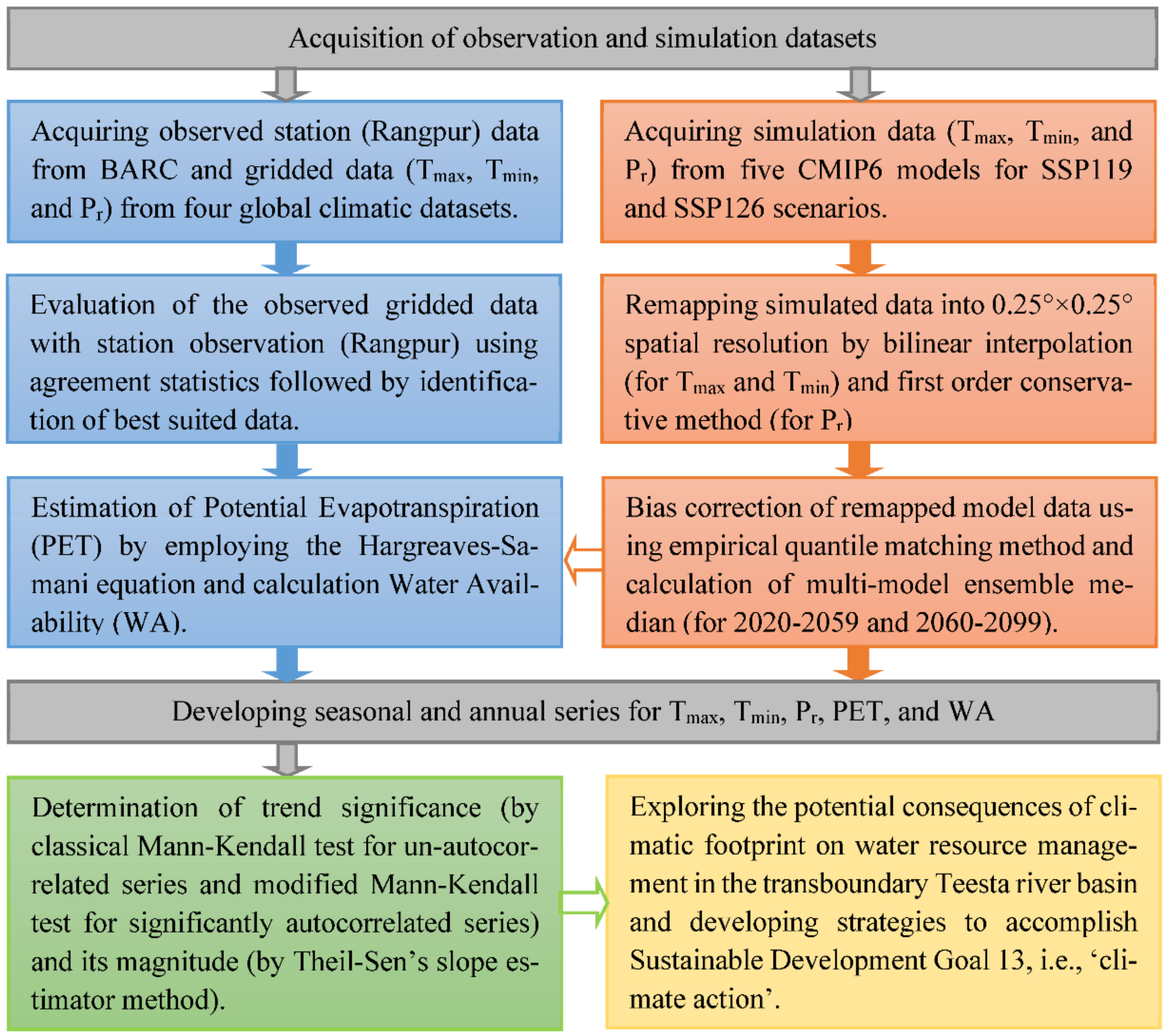
3. Materials and Methods

3.1. Data Type and Source

The study is based on both the observed and simulation data. All data were analyzed at the seasonal and annual scales. Considering the basin’s geographical location, the seasonal data were calculated for four seasons, namely, pre-monsoon (March–May), monsoon (June–September), post-monsoon (October–November), and winter (December–February). The study considered annual scale, keeping in mind the lengthy procedure of the climatic changes. Seasonal data were opted for since the changes in trend might differ from season to season [22]. At the same time, a significant rising trend that occurred on a yearly scale might also result in a not-significant falling trend in seasonal scales [23].

3.1.1. Observational Data

As we intended to explore the changes in the entire basin’s climate shared by India and Bangladesh, we looked for a fine resolution dataset that covers the entire spatial extents. For this purpose, the gridded monthly temperature (Tmax and Tmin) and precipitation data were acquired from the Climate Research Unit Time Series (CRU TS), the Global Meteorological Forcing Dataset for land surface modeling developed by Princeton University (in short, Princeton Global Forcing (PGF) dataset), ERA5, and Indian Monsoon Data Assimilation and Analysis (IMDAA) (Table 2). The first three datasets are extensively used in different climatological studies in India [24,25,26], and several studies [27,28,29] reported a good agreement with India Meteorological Department (IMD) station observations. The IMDAA is a finer-resolution (0.12° × 0.12°) recent reanalysis product carried out for the Indian subcontinent. Various aspects regarding the IMDAA data, e.g., quality control, bias correction, data assimilation, land surface analysis, and verification of reanalysis products, can be found in the study of Rani et al. [30]. These observational data were converted into the seasonal and annual scale and validated against the station data of Rangpur, Bangladesh (acquired from the Bangladesh Agricultural Research Council; Figure 1a). However, the observational datasets were of different periods, and to provide an equal chance for each, the period of 1981–2010 was selected for the assessment.

3.1.2. Simulation Data

The precipitation and maximum and minimum temperatures at the monthly scale from five CMIP6 GCMs were obtained from https://esgf-node.llnl.gov/search/cmip6/ (accessed on 21 October 2021). Details of the selected GCMs are presented in Table 2.
The selected GCMs have both the temperature and rainfall simulations for SSP119 and SSP126 and have been used in some of the recent studies conducted over the South Asian region, in which the performance of these data is found to be satisfactory [31,32,33]. Moreover, these GCMs have considerably improved in terms of their horizontal resolution in comparison to the CMIP5 models. Additionally, the dynamical representation and parameterization schemes have been upgraded to produce more reliable climatic simulations [34].
Table 2. Details of the observation and simulation data used in this study.
Observation DataSource InstitutionSpatial ResolutionReference
StationRangpurBangladesh Agricultural Research Council (BARC)[35]
GriddedCRU TS v4.05University of East Anglia, UK0.5° × 0.5°[36]
PGFPrinceton University, New Jersey0.25° × 0.25°[37]
ERA5European Centre for Medium-Range Weather Forecasts, UK0.25° × 0.25°[38]
IMDAAA collaborative effort among the Met Office, UK, the National Centre for Medium Range Weather Forecasting, India and the India Meteorological Department0.12° × 0.12°[30]
CMIP6 ModelModeling CenterSpatial ResolutionReference
SimulationCanESM5Canadian Centre for Climate Modelling and Analysis, Canada2.8° × 2.8°[39]
GFDL-ESM4Geophysical Fluid Dynamics Laboratory, National Oceanic and Atmospheric Administration, USA1.3° × 1°[40]
IPSL-CM6A-LRInstitut Pierre-Simon Laplace, Sorbonne Université, France2.5° × 1.3°[41]
MIROC6Atmosphere and Ocean Research Institute, The University of Tokyo, Japan1.4° × 1.4°[42]
MRI-ESM2-0The Meteorological Research Institute, Japan2.8° × 2.8°[43]

3.2. Methodology

3.2.1. Performance Evaluation

In order to validate the gridded temperature and precipitation data against station-based observation, we used five different widely recognized agreement statistics. These are as follows.

Pearson Correlation Coefficient (R)

It is a metric for determining the linear strength of associations between two variables, which is computed by dividing the covariance of the two variables by the product of their standard deviations (Equation (1)). The R ranges between −1 and 1, where 1 (−1) denotes perfect positive (negative) correlation and 0 indicates a neutral association [44].
R = i = 1 n ( x i x ¯ ) ( y i y ¯ ) i = 1 n ( x i x ¯ ) 2 i = 1 n ( y i y ¯ ) 2

Coefficient of Determination (R2)

In general, the R2 determines how well the model data are fitted to observation data. It is calculated as the square of the Pearson correlation coefficient (Equation (2)). The value of R2 ranges from 0 to 1 and is usually expressed in percentage. The closer the value of R2 to 1, the better the model [45].
R 2 = i = 1 n ( x i x ¯ ) ( y i y ¯ ) i = 1 n ( x i x ¯ ) 2 i = 1 n ( y i y ¯ ) 2 2

Normalized Root Mean Squared Error (nRMSE)

The nRMSE is nothing but the normalization of RMSE (mean difference between observed and modeled data), which was computed using the mean of the observed data (Equation (3)). Such normalization helps to compare between datasets with different scales [46]. The nRMSE values are often expressed in percentage, where a lower value means less variance and is thus considered better.
n R M S E = i = 1 n ( x i y i ) 2 / n x ¯

Mean Bias Error (MBE)

It can indicate whether the model data overestimate or underestimate the actual data through capturing the average biases in the prediction and is calculated using Equation (4). A positive value of MBE indicates that the gridded data are overestimated from observation data, and vice versa [47].
M B E = 1 n i = 1 n ( y i x i )

Index of Agreement (IOA)

According to Willmott [48], IOA is the ratio of the mean square error and the potential error (Equation (5)). It can capture the additive and proportional differences in the actual and modeled means and variances, albeit sensitive to extreme values. The output ranges from 0 and 1, where 1 indicates a perfect match, and 0 denotes no agreement at all.
I O A = 1 i = 1 n ( x i y i ) 2 i = 1 n y i x ¯ + x i x ¯ 2
where x, y, x ¯ , and y ¯ are the observed data, gridded data, and their respective means. n is the number of observations.

3.2.2. Bias Correction of the GCM Outputs

The spatial resolution of all the CMIP6 GCMs was not similar. Therefore, we re-gridded the data into a common spatial resolution of 0.25° × 0.25°. The bilinear interpolation technique was used to remap the temperature data. This technique is widely applied in different studies for remapping as it does not alter the climate signal [49]. However, for the precipitation, the first-order conservative method was used [50]. This method is particularly suitable for remapping the discontinuous variables such as precipitation [51].
The meteorological variables obtained from the GCMs are well known to exhibit biases [49]. The limited spatial resolution and simplified physics and thermodynamics cause systemic errors in the models, which are generally responsible for biases [15]. As a result, these outputs must be bias-corrected to generate valid estimates at regional and local scales. In this study, we applied the empirical quantile mapping (EQM) method, which is a non-parametric cumulative distribution function (CDF) transformation technique and has performed better in eliminating systematic biases from GCM outputs compared to that of parametric approaches [49,52]. We took the 1971–2010 period to obtain the transformation function (empirical CDF) to map the distribution of model data to observed data [53,54,55]. The CDFs were estimated using empirical percentiles, and values in between the percentiles were approximated using linear interpolation [52]. If the model values from GCMs are larger (smaller) than the training values used to estimate the empirical CDF, the correction found for the highest (lowest) quantile of the training period was used [49,53,54].

3.2.3. Estimation of Potential Evapotranspiration (PET)

We used the Hargreaves–Samani (H-S) equation to estimate the PET. This method is more robust as it avoids overestimation of PET values by methods based on mean temperatures, such as the Thornthwaite method [56]. The study of Rajabi and Babakhani [57] reported that the estimated PET values by the H-S method are closer to the Penman–Monteith FAO (PM FAO). However, the applicability of the PM FAO equation, especially in developing countries, is limited because of the high input data and complexity of the model [58,59]. The H-S method needs only average, minimum, and maximum temperature and solar radiation as input to estimate the PET [60]. In the recent past, several studies [61,62] used the H-S equation (Equation (6)) to estimate the PET throughout the world. It is expressed as follows.
P E T = 0.0023 ( T mean + 17.8 ) ( T max T min ) 0.5 R a
where Tmean, Tmax, and Tmin are the mean, maximum, and minimum air temperature in °C, respectively. Ra is the extraterrestrial radiation (MJ m−2 day−1) estimated using Equation (7).
R a = 24 × 60 π × G s c . d r ω s sin ( ϕ ) sin ( δ ) + cos ( ϕ ) cos ( δ ) sin ( ω s )
where Gsc is a solar constant (0.0820 MJ m–2 min–1), dr is the inverse relative distance of Earth–Sun, ωs is the sunset hour angle (in radians), ϕ is the station latitude (in radians), and δ is the solar declination (in radians). Note that R a d i a n s = π / 180   d e c i m a l   d e g r e e s . The values of dr, δ, and ωs were calculated using the following methods (Equations (8)–(10)), as recommended by Allen et al. [63].
d r = 10.033 cos 2 π 365 J
δ = 0.409 sin 2 π 365 J 1.39
ω s = arccos [ tan ( ϕ ) tan ( δ ) ]
where J refers to the number of days in the year between 1 (1 January) and 365 or 366 (31 December).

3.2.4. Calculation of Water Availability (WA)

In this study, the balance between precipitation (Pr) and PET was used to estimate the net water available (NWA) in the entire basin area. The NWA (Equation (11)) can be considered as the total available water that can be in the form of runoff, soil moisture, and groundwater recharge in the basin area [62].
N W A = P r P E T

3.2.5. Detection of Trend and its Magnitude

In this study, a significant trend in meteorological series is determined by the Mann–Kendall (MK) test, whereas its magnitude is estimated using Theil–Sen’s slope estimator. Both of these techniques are non-parametric and have been applied by several researchers. Even the non-parametric MK test is recommended by the World Meteorological Organization (WMO) owing to its compatibility with non-normalized data as well as missing values [64]. However, the presence of positive autocorrelation in the time series enhances the possibility of detecting trends while there is no trend, and vice versa [65]. Therefore, all data were statistically tested (at a 95 percent confidence interval) for a significant autocorrelation coefficient. In this study, the modified Mann–Kendall (MMK) test, as proposed by Hamed and Rao [65], was used to detect the trend of a significant auto-correlated time series.

The Mann–Kendall (MK) test

The MK test statistic [66,67] is calculated from the sum of the signs (+ or −) of the slopes. The statistic S is expressed in Equation (12).
S = a = 1 n 1 b = a + 1 n sgn x b x a
where (b > a) and n is the number of data points, Xb is the bth observation, and Xa is the ath observation. The sgn (XbXa) is an indicator function that takes on the values 1, 0, or −1 according to the sign of (XbXa) expressed in Equation (13)
sgn x b - x a = 1   if x b x a >   0 0   if x b x a = 0 1   if x b x a <   0
when n ≥ 10, the statistic S is approximately normally distributed with the mean E(S) = 0, and the variance can be obtained by Equation (14).
V ( S ) = n n 1 2 n + 5 k = 1 q t k 1 2 t k + 1 18
where q is the number of ties in the series; tk is the number of data points in the kth tied group. Then, the S and V(S) are used to calculate the test statistic Z, which is stated in
Z = S     1 Var ( S ) 1 / 2 if   S   >   0 0 if   S   =   0 S   +   1 Var ( S ) 1 / 2 if   S   <   0
The trend is said to be decreasing (increasing) if Z is negative (positive). The null hypothesis (H0) of no trend will be rejected if the absolute value of Z is greater than Z 1 α   / 2 , where Z 1 α   / 2 is acquired from the standard normal cumulative distribution tables.

Theil–Sen slope estimator (TSSE)

If a linear trend exists in a time series, the slope or magnitude of that trend can be detected using a simple non-parametric procedure first developed by Theil [68] and later modified by Sen [69]. The slope estimates (Qi) of N data pairs are computed using Equation (16).
Q i = x b x a b a   where   ( b   >   a )
where Xb and Xa are the data values at times b and a, respectively. The median of these N values of Qi is Sen’s estimator of a slope, while the sign of the slope directs data trend reflection.

Modified Mann–Kendall (MMK) test

The MMK test proposed by Hamed and Rao [65] is based on the modified variance expressed in Equation (17).
V * ( S ) = V ( S ) n n * S
where V(S) is the same used in the MK test. The autocorrelation between the ranks of the observations (Pk) is first evaluated using a similar formula as adopted by Datta and Das [22]. The values of Pk were calculated after subtracting the slope parameter by using Equation (16) from the respective time series. The non-significant values of Pk can badly affect the precision of the variance of S, and thus, only significant Pk values were opted to estimate, n/n*S, expressed in Equation (18).
n n * S = 1 + 2 n ( n 1 ) ( n 2 ) × k = 1 n 1 ( n k ) ( n k 1 ) ( n k 2 ) p k
where n is the actual number of observations, n*S is considered as an effective sample of observations. In this study, all lags are considered to obtain a significant autocorrelation coefficient, as suggested by Hamed and Rao [65]. The entire methodological flowchart followed in this study is presented in Figure 2.

4. Results

4.1. Performance Evaluation of the Gridded Observation Data

While evaluating the performance of the gridded data with respect to the station data of Rangpur, Bangladesh, the Princeton Global Forcing (PGF) dataset performed better in comparison to all other datasets (see Supplementary Table S1a–c). CRU TS and ERA5 underestimated the station observation data for the Tmax, whereas the PGF and IMDAA data slightly overestimated. On the other hand, the CRU TS data highly underestimated the Tmin data of Rangpur than the other three datasets. It should be noted that the PGF data consistently outperformed the other three datasets across all statistical indices in the case of Tmin. Considering the precipitation, PGF, CRU TS, and ERA5 datasets slightly underestimated the observed station data. In contrast, the IMDAA data highly overestimated the rainfall. Considering the R, R2, nRMSE, and IOA efficiency statistics, the PGF data performed quite well. Except for the pre-monsoon and post-monsoon, both the R and R2 are higher in the PGF dataset. The nRMSE is lowest in all the seasons except post-monsoon, and the IOA is highest in every season except post-monsoon.

4.2. Performance of the Bias-Corrected CMIP6 Model Data

The performance of the bias-corrected CMIP6 model data against the PGF data for the reference/observed period of 1971–2010 is presented in Supplementary Table S2a–o. For the Tmax and Tmin data, all the five models show a higher R value, which is typically above 0.84, and even in some cases, it reached 1, indicating a very high correlation with the reference period. The R2 values are also more than 0.90 in most grid points in all the models. The nRMSE values for the Tmax varied from 1.30 to −1.29, 0.94 to −0.92, 1.14 to −1.14, 1.45 to −1.47, and 0.98 to −0.98 for the CanESM5, GFDL-ESM4, IPSL-CM6A-LR, MIROC6, and MRI-ESM2-0, respectively. For the Tmin, the nRMSE varied from 1.44 to −1.98, 1.19 to −1.87, 1.1 7to −1.84, 1.46 to −2.12, and 1.36 to −1.84 for the CanESM5, GFDL-ESM4, IPSL-CM6A-LR, MIROC6, and MRI-ESM2-0, respectively. The MBE values are 0 in all the models for both the Tmax and Tmin, which denotes that the EQM method performed well in eliminating the biases from the models. The values for the IOA are closer to 1 and even 1 for many grids, indicating a higher agreement of the bias-corrected results with the gridded observation (PGF) data.
For the precipitation, the R values are mostly above 0.90 in all the models, and the R2 values are also ≥0.90 in all the models, except for the CanESM5, where some grids showed R2 values less than 0.90 and varied from 0.81 to 0.93. The nRMSE ranged from 1.62 to 1.03, 1.13 to 0.87, 1.16 to 0.70, 1.06 to 0.83, and 1.19 to 0.64 for the CanESM5, GFDL-ESM4, IPSL-CM6A-LR, MIROC6, and MRI-ESM2-0, respectively. Both the positive and negative biases are observed in the CanESM5, GFDL-ESM4, and IPSL-CM6A-LR models. The IPSL-CM6A-LR model showed the highest number of grids with negative biases. However, the MIROC6 and MRI-ESM2-0 exhibited only positive biases. Nevertheless, all the models performed quite well in terms of the IOA, where the values are mostly above 0.90 and close to 1.

4.3. Trends and Trend Magnitudes in Temperature (Tmax and Tmin)

Trends and their magnitudes of the Tmax and Tmin across the Teesta river basin for the observed period and at the 1.5 and 2 °C warming scenarios are demonstrated in Figure 3 and Figure 4. In general, both Tmax and Tmin increased throughout the basin area during the observed period (1971–2010). The highest rate of increase was found in the winter (0.029 °C/year for Tmax and 0.043 °C/year for Tmin), and the lowest in the post-monsoon season (0.013 °C/year for Tmax and 0.012 °C/year for Tmin). The Tmax was significantly increasing during the monsoon season in the central and lower parts of the basin. On the other hand, the Tmin increased throughout the basin during pre-monsoon, monsoon, and annual series. However, in winter, it was significantly increasing only in the upper parts of the basin. Meanwhile, it should be noted that the Tmin was rising at a faster rate than the Tmax.
In the near future (2020–2059) of the two projected scenarios, both the Tmax and Tmin were mostly increasing. In the near future of SSP119, the increase in Tmax was significant during the pre-monsoon, monsoon, and annual scale in the upper parts of the basin, and in the case of Tmin, the warming was significant only during the monsoon and annual scale throughout the basin area. For Tmax, the highest increase was observed in the winter (0.020 °C/year) at the lower parts of the basin, and for Tmin, in the post-monsoon (0.021 °C/year) season at the upper parts of the basin. Considering the near future of the SSP126 scenario, the post-monsoon season showed the highest rate of increase both in Tmax (0.019 °C/year) and Tmin (0.053 °C/year). In contrast, considering the far future (2060–2099), Tmax and Tmin decreased in both scenarios. It is worth mentioning that the decreasing trends showed higher magnitudes for the SSP119 than SSP126 in the far future (2060–2099).

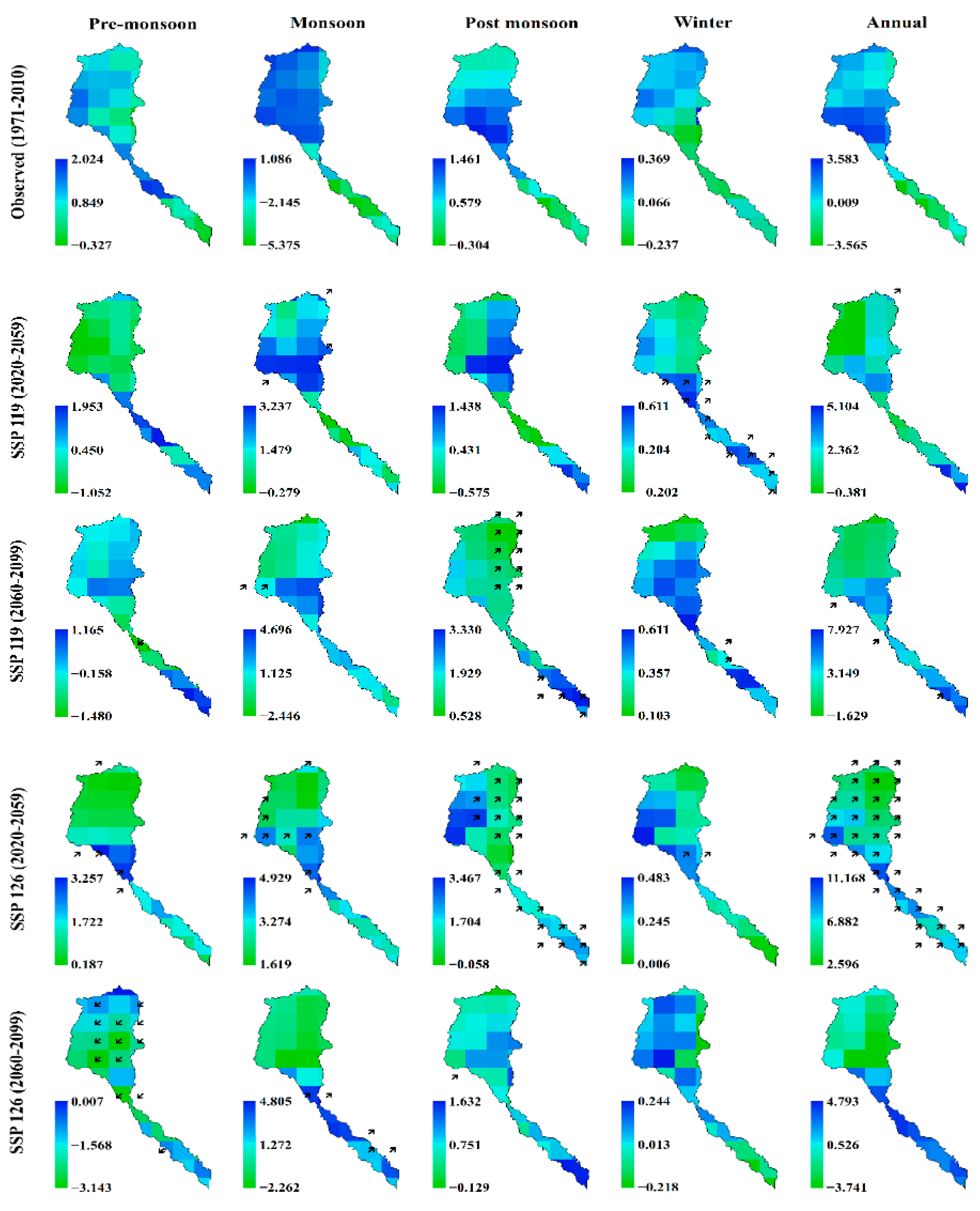
4.4. Trends and Trend Magnitudes in the Precipitation

Figure 5 illustrates the trends and their magnitudes of the precipitation across the Teesta river basin for the observation period and two SSP scenarios. There was no significant trend in the entire basin during the observed period (1971–2010). However, in most of the lower parts (upper parts) of the basin, the negative (positive) trend was consistent in every season.
Considering the near future (2020–2059) in SSP119, there was a significant increasing trend in the lower parts of the basin during the winter, and some scattered significant increasing trends were found in the upper part of the basin during the monsoon season. The highest trend magnitudes during this period were observed during the annual (5.104 mm/year) and monsoon season (3.237 mm/year). In the far future (2060–2099), precipitation mostly increased significantly, except during the pre-monsoon season. Maximum significant increasing trends were seen in the post-monsoon season. Similar to the near future, the highest trend magnitude was found in the annual (7.927 mm/year) and monsoon season (4.696 mm/year); nevertheless, the magnitude was much higher in the far future. However, in both periods of SSP119, higher trend magnitudes were mostly observed in the lower parts of the basin.
There was an overall increase in precipitation in the near future of SSP126. Most of the significant increasing trends were found during the annual and post-monsoon season. In the far future, a few significant increasing and decreasing trends were observed, mostly in the monsoon and pre-monsoon seasons, respectively. The lower parts of the Sikkim showed the highest decrease (−3.143 mm/year) in the pre-monsoon season. On the other hand, the highest rate of increase was detected in the monsoon and annual series in both the near (4.929 mm/year in monsoon and 11.168 mm/year in annual) and far future (4.805 mm/year in monsoon and 4.793 mm/year in annual) of SSP126.

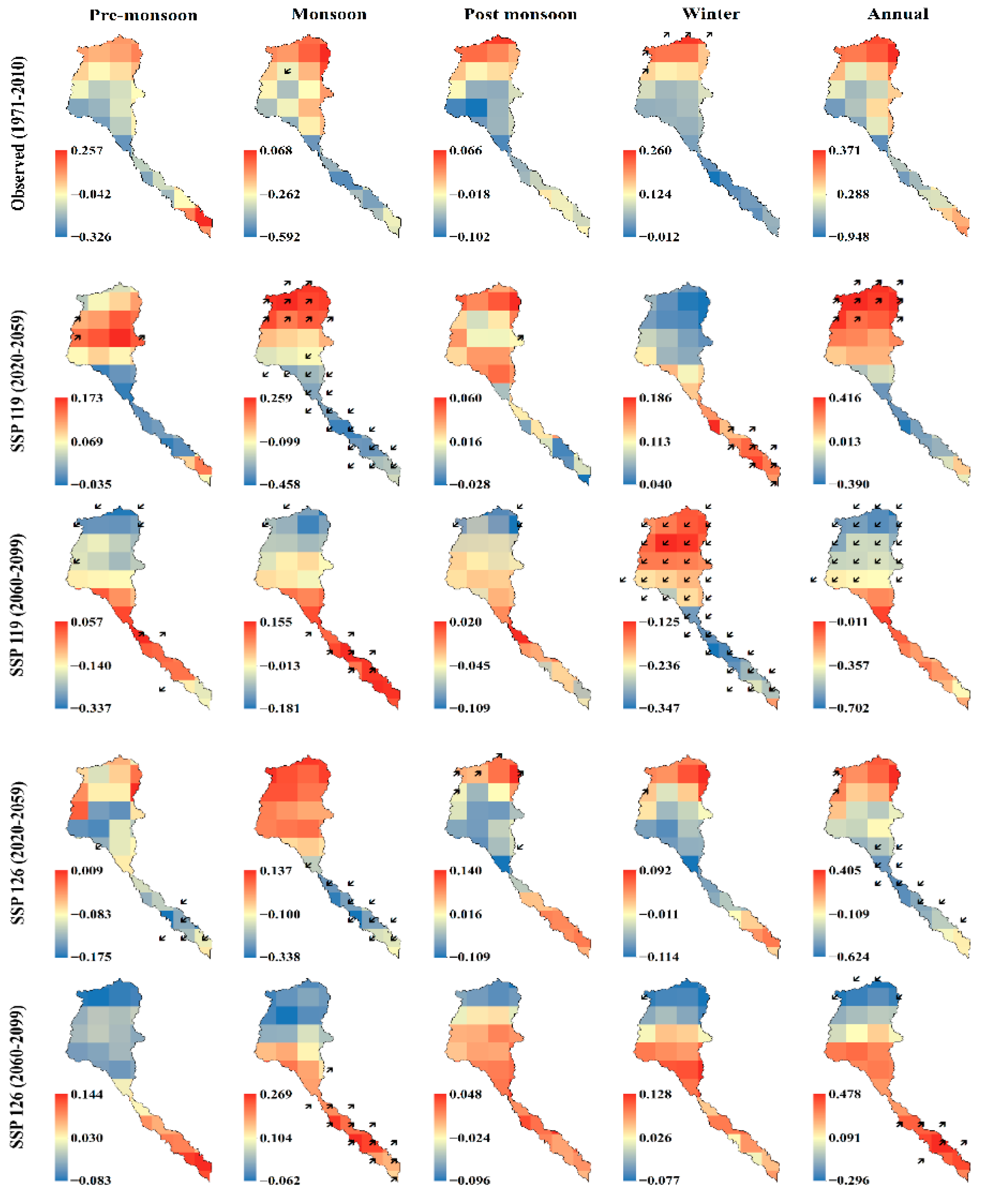
4.5. Trends and Trend Magnitudes in the Potential Evapotranspiration (PET)

The trends and magnitudes in PET for the observed period and 1.5 and 2 °C warming levels are presented in Figure 6. Both the increasing and decreasing trends of PET were noticed; however, these were mostly not significant throughout the basin, except during the winter and monsoon seasons. In winter, some significant increasing trends were witnessed in the upper parts of the basin, whereas in monsoon season, only one grid showed a significant decreasing trend. The higher magnitudes were mostly seen in the upper parts of the basin. However, the lower parts of the basin also showed higher magnitudes in the pre-monsoon and annual series, albeit statistically not significant.
In the near future of SSP119, significant increasing trends were mostly observed in the upper parts of the basin during the monsoon and annual scales. In the winter, significant increasing trends were found in the lower parts of the basin. Significant decreasing trends were visible in the central and lower parts of the basin during the monsoon season. Both the highest and lowest trend magnitudes were observed in the monsoon season, which varied from 0.259 mm/year to −0.458 mm/year. On the other hand, the far future of SSP119 also depicted both the significant increasing and decreasing trends. Significant decreasing trends were prominent throughout the basin in the winter season, whereas in other seasons, quite a few grids with significant negative and positive trends were noticed in the uppermost and lower part of the basin, respectively. The annual series showed only significant decreasing trends in the upper parts of the basin. The highest decrease (0.347 mm/year) and increase (0.155 mm/year) was witnessed in the winter and monsoon season, respectively.
Considering the near future of the SSP126, significant decreasing trends were mostly observed in the central and lower parts of the basin, except during the post-monsoon and winter seasons. The highest decrease (−0.338 mm/year) was in the monsoon season, which is quite similar to the near future of SSP119. A few grids with significant increasing trends were seen in the upper parts on the post-monsoon, winter, and annual scales. Contrary to this, in the far future, significant increasing trends were found in the lower parts of the basin during the monsoon season, including the annual series. Very few grids with significant decreasing trends were detected in the upper parts of the basin in the winter and annual scales.

4.6. Trends and Trend Magnitudes in the Water Availability (WA)

There is no significant trend in WA during the observed period (Figure 7). However, an overall drying (wetting) pattern was observed at the lower (upper) parts of the basin in the monsoon and post-monsoon season, including the annual series. In the near future of SSP119, we did not find any significant changes in WA within the basin areas. In the far future, significant wetting trends are found in all seasons, except for the pre-monsoon. The rate of increase in WA was prominent in the post-monsoon (varied from 0.652 to 3.460 mm/year) and winter season (varied from 0.189 to 0.955 mm/year).
In almost the entire Teesta river basin, wet patches were predominant in the near future of SSP126. Significant increasing trends were observed in all seasons, except for the winter. The post-monsoon season showed the highest number of grids with significant increasing trends throughout the basin except for the central parts, whereas during pre-monsoon and monsoon seasons, increasing trends were significant in the central parts of the basin. In the far future of SSP126, significant decreasing trends in the WA were prevalent only in the pre-monsoon season, and some scattered significant increasing trends were noticed in the lower middle parts of the basin during the monsoon season. Considering both the periods of SSP126, the highest trend magnitude of 5.367 mm/year was detected in the monsoon season of the near future. In general, the trend magnitudes of WA were relatively lower in the far future than in the near future.

5. Discussion

The results of this study indicate that in both SSPs, the temperature is expected to increase in the near future, whereas some significant decreasing trend is observed in the far future. This finding is quite consistent with the previous study of You et al. [70], who also reported a decreasing temperature trend over China after the 2040s under the SSP126 scenario. Significant increasing trends in the upper parts of the basin are found in the near future under both scenarios. The upper part of the basin area consists of more than 26 glaciers and a number of glacial lakes and water bodies [71]. The enhanced future warming over this region is likely to accelerate the snow melting and, consequently, glacier recession. Such incidents are already reported in the study of Raina [71], which indicated that most of the recessions took place between 1988 and 2005, and the intensity was higher in the post-2000 period. In addition to this, it has also been reported by Agrawal and Tayal [72] that the Rathong glacier, which fed the main tributary (Rangit) of Teesta, has witnessed a decrease of approximately 20 percent of its ice volume from 1962 to 2011. Furthermore, our study showed that in the near future, the monsoon and post-monsoon and in the far future, pre-monsoon and winter precipitation under both SSPs are likely to increase over the upper part of the basin, which, along with the glacier melted water, can trigger floods and flash floods over the basin and might also intensify the existing political turmoil downstream. An overall increase in precipitation under 1.5 and 2 °C warming is also reported in other studies conducted over South Asian regions [31,73].
With the increasing trends in temperature, the study observed a number of decreasing PET trends in the near future, which is more significant in SSP126 than in the SSP119 scenario. This result indicates the existence of the evaporation paradox over the Teesta river basin, especially in the lower reach. A similar kind of result was also observed by Basso et al. [74] in the U.S. Midwest. The study further elaborated that the increase in Tmin was much higher than Tmax (which also concurs with our finding), and this translated into a net reduction in vapor pressure deficit and in turn, a decreased PET. Such increasing Tmin can also affect crop production by altering plant respiration rates and responses to biotic stressors. In the case of WA, it is observed that the basin areas which are showing an increasing trend in temperature and PET, with a decreasing (increasing) trend in precipitation, are likely to experience a decrease (increase) in WA. Moreover, in the areas where PET is decreasing with an increase in precipitation, there would be an increase in WA. Overall, the WA is most likely to increase in the near future, especially in the post-monsoon season under SSP126. However, for the winter season, there is no significant change in WA in the near future. In the far future, the WA is likely to increase at the lower part of the basin under SSP119; however, there is a drying tendency over this region under SSP126, with an exception in the monsoon season.
Considering the near future scenarios of both the SSPs, an expansion of irrigation might be needed since the High Yield Variety (HYV) Boro rice (native Bengali language name of a typical wet variety of paddy sown in winter and harvested in the summer season) is cultivated widely (from November to May) in the central (66.5%) and lower course (81.2%) of the basin areas, which requires a high amount of water supply [75]. In addition to this, the coarse soil texture (mainly sandy to sandy loam) of this region increases the likelihood of seepage, and as a result, the demand for irrigable water becomes higher. Imperatively, the farmers of the lower reach completely rely on groundwater for irrigation in the dry season [76]. Therefore, further expansion of irrigation areas might lead to a substantial decline in groundwater levels in the near future. Such an alarming indication is already witnessed in the lower and central parts of the basin [21,76]. Even though two barrages, Gajoldoba (in India) and Dalia (in Bangladesh), were constructed for irrigational and hydropower generation over the basin area, no storage was constructed to retain and release excess monsoon water for the dry season irrigation [21]. Additionally, numerous hydropower projects at the upper (Sikkim) and central courses (West Bengal) and then linking the Gajoldoba barrage with Siliguri Municipal Corporation (SMC, the third-largest urban agglomeration and the second most important trade hub of the Indian State of West Bengal after Kolkata) to meet the domestic water demand have again stimulated water stress in the downstream areas [75]. Therefore, it might cause a reduction in the dry season’s water availability in the downstream basin areas of Bangladesh, which is already a drought-prone area [12].

6. Conclusions and Way Forward

The present study used the latest CMIP6 scenarios from six GCMs (which have been widely applied in the South Asian context) to quantify the near (2020–2059) and far future (2060–2099) trends and their magnitudes in temperature, precipitation, potential evapotranspiration, and water availability across the transboundary Teesta river basin. The study explicitly utilized two SSP scenarios, SSP119 and SSP126, to portray the expected climatic changes under 1.5 and 2 °C warming, which is also a target set by the Paris Agreement. To improve the accuracy of the CMIP6 GCMs, we applied the non-parametric EQM method, and it performed well in eliminating the existing biases from the CMIP6 models. The historically observed precipitation and temperature (Tmax and Tmin) data from the Princeton Global Forcing (PGF) dataset were used to bias-correct the future CMIP6 model data. The PGF data performed well amongst the selected global level gridded datasets while evaluating the performance with the station observation record of Rangpur, Bangladesh. We used the ensemble median to report the results since GCM ensembles provide more reliable estimates than the single models [17,77]. The bias correction and multi-model ensembles of the GCM outputs are, therefore, capable of providing more accurate representativeness by decreasing spatial ambiguity and inconsistency [73].
Undoubtedly, the Teesta river holds immense importance both for the India and Bangladesh. However, climate change has added a new dimension to the existing political and eco-hydrological issues of the basin. Although the future scenarios are projecting an overall increase in water availability, it should also be mentioned that in the near future, the magnitude of warming is much more in SSP126 than in SSP119, and in the far future, even though there is a decreasing trend in temperature, the decrease is much lesser in SSP126 than in SSP119. Such rising temperature under the SSP126 scenario at the upper course of the Teesta river basin might even hinder the glaciation process and escalate snow melt, which will inevitably accelerate the river discharge in the short term but reduce in the long term. Therefore, limiting the warming by 1.5 °C might be more appropriate. Presently, both the riparian countries have set their Nationally Determined Contributions (NDCs) to reduce greenhouse gas (GHG) emissions. However, focusing solely on mitigation would not be sufficient for sustainable development, and thus, adaptation strategies to changing climatic conditions are also required and should be implemented concurrently with mitigation strategies.
Considering the present and future climatic conditions of the Teesta river basin as well as its socioeconomic and geopolitical relevance, both the co-riparian nations should prioritize the 13th Sustainable Development Goal (SDG) “Climate Action”, especially the target 13.2, i.e., “integrate climate change measures into national policies, strategies and planning”. In order to achieve this goal, we propose a combination of long- and short-term strategies based on the obtained results to guide policymakers in implementing the SDG framework in this region. These are as follows:
  • For a long-term solution, both the riparian countries should reinitiate the dialogue process of the Joint River Commission (JRC, a bilateral working group established by India and Bangladesh in 1972 for the Indo-Bangla Treaty of Friendship, Cooperation and Peace) to avoid water disputes and strengthen the mutual cooperation for controlling floods and tackling the water crisis. Apart from this, both nations could build reservoirs over the river basin to store the excess monsoonal rainfall and connect them with the existing canal network to meet the irrigational demands, especially during the lean period.
  • For immediate or short-term actions, both the countries might follow optimal water use and conservation (like rainwater harvesting) through community-driven participatory management and discourage the wet variety of Boro paddy cultivation by encouraging drought-tolerant cash crops. Having said that, if the total volume of irrigable water is utilized for the other winter crops instead of Boro, then at most, 45,000 ha of land could be irrigated [21].
  • Excavation of deep farm ponds is also an alternative and economical path not only to store rainwater but also meaningful to mitigate sudden floods. At the same time, it is capable of replenishing groundwater and soil moisture levels.
Implementation of these strategies would offset the local level risks, and in consequence, the communities would be in a better position to support the overall conservation of the river to keep the basin ecologically healthy and environmentally sustainable. In this regard, adopting cooperative behaviors among different stakeholders of the riparian countriescould play an important role in disseminating the required technical know-how and providing access to different capital assets, which would eventually help establish blue peace over the transboundary Teesta river basin.

Supplementary Materials

The following supporting information can be downloaded at: https://www.mdpi.com/article/10.3390/atmos13060941/s1, Table S1a: Performance evaluation of the observed gridded data with respect to station data for the Tmax, Table S1b: Performance evaluation of the observed gridded data with respect to station data for the Tmin, Table S1c: Performance evaluation of the observed gridded data with respect to station data for the precipitation, Table S2a: Evaluation of bias-corrected Tmax data of CanESM5 for the reference period of 1971–2010, Table S2b: Evaluation of bias-corrected Tmin data of CanESM5 for the reference period of 1971–2010, Table S2c: Evaluation of bias-corrected precipitation data of CanESM5 for the reference period of 1971–2010, Table S2d: Evaluation of bias-corrected Tmax data of GFDL-ESM4 for the reference period of 1971–2010, Table S2e: Evaluation of bias-corrected Tmin data of GFDL-ESM4 for the reference period of 1971–2010, Table S2f: Evaluation of bias-corrected precipitation data of GFDL-ESM4 for the reference period of 1971–2010, Table S2g: Evaluation of bias-corrected Tmax data of IPSL-CM6A-LR for the reference period of 1971–2010, Table S2h: Evaluation of bias-corrected Tmin data of IPSL-CM6A-LR for the reference period of 1971–2010, Table S2i: Evaluation of bias-corrected precipitation data of IPSL-CM6A-LR for the reference period of 1971–2010, Table S2j: Evaluation of bias-corrected Tmax data of MIROC6 for the reference period of 1971–2010, Table S2k: Evaluation of bias-corrected Tmin data of MIROC6 for the reference period of 1971–2010, Table S2l: Evaluation of bias-corrected precipitation data of MIROC6 for the reference period of 1971–2010, Table S2m: Evaluation of bias-corrected Tmax data of MRI-ESM2-0 for the reference period of 1971–2010, Table S2n: Evaluation of bias-corrected Tmin data of MRI-ESM2-0 for the reference period of 1971–2010, Table S2o: Evaluation of bias-corrected precipitation data of MRI-ESM2-0 for the reference period of 1971–2010.

Author Contributions

Conceptualization, S.D. and P.D.; methodology, S.D., P.D., D.S. and K.G.; software, S.D.; formal analysis, S.D.; investigation, P.D. and S.D.; resources, S.D.; data curation, S.D. and P.D.; writing—original draft preparation, S.D. and P.D.; writing—review and editing, D.S. and K.G. All authors have read and agreed to the published version of the manuscript.

Funding

This research received no external funding.

Institutional Review Board Statement

Not applicable.

Informed Consent Statement

Not applicable.

Data Availability Statement

The data reported in this study are available within the manuscript and in the Supplementary Materials.

Acknowledgments

We would like to acknowledge MDPI for working on the SDG Publishers Compact and providing us with the opportunity to be a part of this project by waiving the article processing charge (APC). The authors would also like to express their gratitude to the Editorial Board members and reviewers for their critical comments and constructive suggestions. A special thanks to the Publishing Manager for the assistance during the entire submission process.

Conflicts of Interest

The authors declare no conflict of interest.

References

  1. Melesse, A.M.; Abtew, W.; Setegn, S.G. (Eds.) Nile River Basin: Ecohydrological Challenges, Climate Change and Hydropolitics; Springer International Publishing: Cham, Switzerland, 2014. [Google Scholar]
  2. Mahmood, R.; Jia, S. Assessment of impacts of climate change on the water resources of the transboundary Jhelum River basin of Pakistan and India. Water 2016, 8, 246. [Google Scholar] [CrossRef] [Green Version]
  3. Barnes, J. The future of the Nile: Climate change, land use, infrastructure management, and treaty negotiations in a transboundary river basin. Wiley Interdiscip. Rev. Clim. Change 2017, 8, 449. [Google Scholar] [CrossRef]
  4. Shamir, E.; Tapia-Villaseñor, E.M.; Cruz-Ayala, M.B.; Megdal, S.B. A review of climate change impacts on the USA-Mexico transboundary Santa Cruz River Basin. Water 2021, 13, 1390. [Google Scholar] [CrossRef]
  5. Soroush, F.; Fathian, F.; Khabisi, F.S.H.; Kahya, E. Trends in pan evaporation and climate variables in Iran. Theor. Appl. Climatol. 2020, 142, 407–432. [Google Scholar] [CrossRef]
  6. Qin, M.; Zhang, Y.; Wan, S.; Yue, Y.; Cheng, Y.; Zhang, B. Impact of climate change on “evaporation paradox” in province of Jiangsu in southeastern China. PLoS ONE 2021, 16, 0247278. [Google Scholar] [CrossRef]
  7. Goyal, M.K.; Goswami, U.P. Teesta river and its ecosystem. In The Indian Rivers; Springer: Singapore, 2018; pp. 537–551. [Google Scholar]
  8. Prasai, S.; Surie, M.D. Transboundary Water Cooperation Key to Easing South Asia’s Water Woes. The Asia Foundation. 20 March 2013. Available online: https://asiafoundation.org/2013/03/20/transboundary-water-cooperation-key-to-easing-south-asias-water-woes/ (accessed on 26 June 2021).
  9. Gambhir, M. Teesta Dispute and India-Bangladesh Relations. 2021. Available online: https://www.claws.in/teesta-dispute-and-india-bangladesh-relations/#_edn6 (accessed on 22 July 2021).
  10. Farinosi, F.; Giupponi, C.; Reynaud, A.; Ceccherini, G.; Carmona-Moreno, C.; De Roo, A.; Gonzalez-Sanchez, D.; Bidoglio, G. An innovative approach to the assessment of hydro-political risk: A spatially explicit, data driven indicator of hydro-political issues. Glob. Environ. Change 2018, 52, 286–313. [Google Scholar] [CrossRef]
  11. Islam, M.F. Water Use and Poverty Reduction; Springer: Tokyo, Japan, 2016. [Google Scholar]
  12. Arfanuzzaman, M.; Syed, M.A. Water demand and ecosystem nexus in the transboundary river basin: A zero-sum game. Environ. Dev. Sustain. 2018, 20, 963–974. [Google Scholar] [CrossRef]
  13. United Nations. UN Convention on the Law of Non-Navigational Uses of International Watercourses. 1997. Available online: https://legal.un.org/ilc/texts/instruments/english/conventions/8_3_1997.pdf (accessed on 5 April 2020).
  14. Soorya, S.; Adarsh, S.; Priya, K.L. Trend analysis of rainfall projections of Teesta river basin, Sikkim using non-parametric tests and ensemble empirical mode decomposition. In Emerging Trends in Engineering, Science and Technology for Society, Energy and Environment; Vanchipura, R., Jiji, K.S., Eds.; CRC Press: Boca Raton, FL, USA, 2018; pp. 103–110. [Google Scholar]
  15. Sharma, A.; Goyal, M.K. Assessment of the changes in precipitation and temperature in Teesta River basin in Indian Himalayan Region under climate change. Atmos. Res. 2020, 231, 104670. [Google Scholar] [CrossRef]
  16. Kumar, D.; Arya, D.S.; Murumkar, A.R.; Rahman, M.M. Impact of climate change on rainfall in Northwestern Bangladesh using multi-GCM ensembles. Int. J. Climatol. 2014, 34, 1395–1404. [Google Scholar] [CrossRef]
  17. Su, B.; Huang, J.; Mondal, S.K.; Zhai, J.; Wang, Y.; Wen, S.; Gao, M.; Lv, Y.; Jiang, S.; Jiang, T.; et al. Insight from CMIP6 SSP-RCP scenarios for future drought characteristics in China. Atmos. Res. 2021, 250, 105375. [Google Scholar] [CrossRef]
  18. Noolkar-Oak, G. Geopolitics of Water Conflicts in the Teesta River Basin. 2017. Available online: https://www.indiawaterportal.org/sites/indiawaterportal.org/files/geopolitics_of_water_conflicts_in_the_teesta_river_basin_gauri_noolkar_oak_2018.pdf (accessed on 16 March 2019).
  19. Peel, M.C.; Finlayson, B.L.; McMahon, T.A. Updated world map of the Köppen-Geiger climate classification. Hydrol. Earth Syst. Sci. 2007, 11, 1633–1644. [Google Scholar] [CrossRef] [Green Version]
  20. Bangladesh Bureau of Statistics (BBS). Bangladesh Data Sheet. 2011. Available online: http://www.bbs.gov.bd/WebTestApplication/userfiles/Image/SubjectMatterDataIndex/datasheet.xls (accessed on 17 August 2016).
  21. Rudra, K. Sharing water across Indo-Bangladesh border. In Regional Cooperation in South Asia: Socio-Economic, Spatial, Ecological and Institutional Aspects (Contemporary South Asian Studies); Bandyopadhyay, S., Torre, A., Casaca, P., Dentinho, T., Eds.; Springer: Cham, Switzerland, 2017; pp. 189–207. [Google Scholar]
  22. Datta, P.; Das, S. Analysis of long-term seasonal and annual temperature trends in North Bengal, India. Spat. Inf. Res. 2019, 27, 475–496. [Google Scholar] [CrossRef]
  23. Nalley, D.; Adamowski, J.; Khalil, B.; Ozga-Zielinski, B. Trend detection in surface air temperature in Ontario and Quebec, Canada during 1967–2006 using the discrete wavelet transform. Atmos. Res. 2013, 132, 375–398. [Google Scholar] [CrossRef]
  24. Datta, P.; Das, S. Analysis of long-term precipitation changes in West Bengal, India: An approach to detect monotonic trends influenced by autocorrelations. Dyn. Atmos. Ocean. 2019, 88, 101118. [Google Scholar] [CrossRef]
  25. Singh, J.; Sahany, S.; Robock, A. Can stratospheric geoengineering alleviate global warming-induced changes in deciduous fruit cultivation? The case of Himachal Pradesh (India). Clim. Change 2020, 162, 1323–1343. [Google Scholar] [CrossRef]
  26. Sedova, B.; Kalkuhl, M. Who are the climate migrants and where do they go? Evidence from rural India. World Dev. 2020, 129, 104848. [Google Scholar] [CrossRef]
  27. Robertson, A.W.; Bell, M.; Cousin, R.; Curtis, A.; Li, S. Online Tools for Assessing the Climatology and Predictability of Rainfall and Temperature in the Indo-Gangetic Plains Based on Observed Datasets and Seasonal Forecast Models; CCAFS Working Papers; CGIAR: Montpellier, France, 2013. [Google Scholar]
  28. Aslam, R.A.; Shrestha, S.; Pal, I.; Ninsawat, S.; Shanmugam, M.S.; Anwar, S. Projections of climatic extremes in a data poor transboundary river basin of India and Pakistan. Int. J. Climatol. 2020, 40, 4992–5010. [Google Scholar] [CrossRef]
  29. Aadhar, S.; Mishra, V. On the occurrence of the worst drought in South Asia in the observed and future climate. Environ. Res. Lett. 2021, 16, 024050. [Google Scholar] [CrossRef]
  30. Rani, S.I.; Arulalan, T.; George, J.P.; Rajagopal, E.N.; Renshaw, R.; Maycock, A.; Barker, D.M.; Rajeevan, M. IMDAA: High-Resolution Satellite-Era Reanalysis for the Indian Monsoon Region. J. Clim. 2021, 34, 5109–5133. [Google Scholar] [CrossRef]
  31. Almazroui, M.; Saeed, S.; Saeed, F.; Islam, M.N.; Ismail, M. Projections of precipitation and temperature over the South Asian countries in CMIP6. Earth Syst. Environ. 2020, 4, 297–320. [Google Scholar] [CrossRef]
  32. Karim, R.; Tan, G.; Ayugi, B.; Babaousmail, H.; Liu, F. Evaluation of historical CMIP6 model simulations of seasonal mean temperature over Pakistan during 1970–2014. Atmosphere 2020, 11, 1005. [Google Scholar] [CrossRef]
  33. Kamal, A.S.M.; Hossain, F.; Shahid, S. Spatiotemporal changes in rainfall and droughts of Bangladesh for 1.5 and 2 °C temperature rise scenarios of CMIP6 models. Theor. Appl. Climatol. 2021, 146, 527–542. [Google Scholar] [CrossRef]
  34. Eyring, V.; Bony, S.; Meehl, G.A.; Senior, C.A.; Stevens, B.; Stouffer, R.J.; Taylor, K.E. Overview of the Coupled Model Intercomparison Project Phase 6 (CMIP6) experimental design and organization. Geosci. Model Dev. 2016, 9, 1937–1958. [Google Scholar] [CrossRef] [Green Version]
  35. Bangladesh Agricultural Research Council. Climate Information Management System. Available online: http://www.barc.gov.bd/ (accessed on 17 January 2022).
  36. Harris, I.; Osborn, T.J.; Jones, P.; Lister, D. Version 4 of the CRU TS monthly high-resolution gridded multivariate climate dataset. Sci. Data 2020, 7, 109. [Google Scholar] [CrossRef] [Green Version]
  37. Sheffield, J.; Goteti, G.; Wood, E.F. Development of a 50-year high-resolution global dataset of meteorological forcings for land surface modeling. J. Clim. 2006, 19, 3088–3111. [Google Scholar] [CrossRef] [Green Version]
  38. Hersbach, H.; Bell, B.; Berrisford, P.; Hirahara, S.; Horányi, A.; Muñoz-Sabater, J.; Nicolas, J.; Peubey, C.; Radu, R.; Schepers, D.; et al. The ERA5 global reanalysis. Q. J. R. Meteorol. Soc. 2020, 146, 1999–2049. [Google Scholar] [CrossRef]
  39. Swart, N.C.; Cole, J.N.; Kharin, V.V.; Lazare, M.; Scinocca, J.F.; Gillett, N.P.; Anstey, J.; Arora, V.; Christian, J.R.; Hanna, S.; et al. The Canadian earth system model version 5 (CanESM5. 0.3). Geosci. Model Dev. 2019, 12, 4823–4873. [Google Scholar] [CrossRef] [Green Version]
  40. Held, I.M.; Guo, H.; Adcroft, A.; Dunne, J.P.; Horowitz, L.W.; Krasting, J.; Shevliakova, E.; Winton, M.; Zhao, M.; Bushuk, M.; et al. Structure and performance of GFDL’s CM4. 0 climate model. J. Adv. Modeling Earth Syst. 2019, 11, 3691–3727. [Google Scholar] [CrossRef] [Green Version]
  41. Boucher, O.; Servonnat, J.; Albright, A.L.; Aumont, O.; Balkanski, Y.; Bastrikov, V.; Bekki, S.; Bonnet, R.; Bony, S.; Bopp, L.; et al. Presentation and evaluation of the IPSL-CM6A-LR climate model. J. Adv. Modeling Earth Syst. 2020, 12, e2019MS002010. [Google Scholar] [CrossRef]
  42. Tatebe, H.; Ogura, T.; Nitta, T.; Komuro, Y.; Ogochi, K.; Takemura, T.; Sudo, K.; Sekiguchi, M.; Abe, M.; Saito, F.; et al. Description and basic evaluation of simulated mean state, internal variability, and climate sensitivity in MIROC6. Geosci. Model Dev. 2019, 12, 2727–2765. [Google Scholar] [CrossRef] [Green Version]
  43. Yukimoto, S.; Kawai, H.; Koshiro, T.; Oshima, N.; Yoshida, K.; Urakawa, S.; Tsujino, H.; Deushi, M.; Tanaka, T.; Hosaka, M.; et al. The Meteorological Research Institute Earth System Model version 2.0, MRI-ESM2. 0: Description and basic evaluation of the physical component. J. Meteorol. Soc. Japan Ser. II 2019, 97, 931–965. [Google Scholar] [CrossRef] [Green Version]
  44. Kanda, N.; Negi, H.S.; Rishi, M.S.; Kumar, A. Performance of various gridded temperature and precipitation datasets over Northwest Himalayan Region. Environ. Res. Commun. 2020, 2, 085002. [Google Scholar] [CrossRef]
  45. Rezaei, M.; Azhdary Moghaddam, M.; Azizyan, G.; Shamsipur, A.A. Assessment of precipitation obtained from gridded data bases in southern Baluchestan basin. Environ. Water Eng. 2022. [Google Scholar] [CrossRef]
  46. Salman, S.A.; Shahid, S.; Ismail, T.; Al-Abadi, A.M.; Wang, X.J.; Chung, E.S. Selection of gridded precipitation data for Iraq using compromise program-ming. Measurement 2019, 132, 87–98. [Google Scholar] [CrossRef]
  47. Ahmed, K.; Shahid, S.; Ali, R.O.; Bin Harun, S.; Wang, X.J. Evaluation of the performance of gridded precipitation products over Balochistan Province, Pakistan. Desalin. Water Treat. 2017, 79, 73–86. [Google Scholar] [CrossRef]
  48. Willmott, C.J. On the validation of models. Phys. Geogr. 1981, 2, 184–194. [Google Scholar] [CrossRef]
  49. Mishra, V.; Bhatia, U.; Tiwari, A.D. Bias-corrected climate projections for South asia from coupled model intercomparison project-6. Sci. Data 2020, 7, 338. [Google Scholar] [CrossRef]
  50. Jones, P.W. First- and second-order conservative remapping schemes for grids in spherical coordinates. Mon. Weather Rev. 1999, 127, 2204–2210. [Google Scholar] [CrossRef]
  51. Saeed, S.; Brisson, E.; Demuzere, M.; Tabari, H.; Willems, P.; van Lipzig, N.P. Multidecadal convection permitting climate simulations over Belgium: Sensitivity of future precipitation extremes. Atmos. Sci. Lett. 2017, 18, 29–36. [Google Scholar] [CrossRef] [Green Version]
  52. Gudmundsson, L.; Bremnes, J.B.; Haugen, J.E.; Engen-Skaugen, T. Downscaling RCM precipitation to the station scale using statistical transformations—A comparison of methods. Hydrol. Earth Syst. Sci. 2012, 16, 3383–3390. [Google Scholar] [CrossRef] [Green Version]
  53. Boé, J.; Terray, L.; Habets, F.; Martin, E. Statistical and dynamical downscaling of the Seine basin climate for hydro-meteorological studies. Int. J. Climatol. 2007, 27, 1643–1655. [Google Scholar] [CrossRef]
  54. Themeßl, M.; Gobiet, A. Empirical-statistical downscaling and model error correction of daily temperature and precipitation from regional climate simulations and the effects on climate change signals. In Proceedings of the EGU General Assembly, Vienna, Austria, 2–7 May 2010; Volume 12, p. 9664. [Google Scholar]
  55. Wetterhall, F.; Pappenberger, F.; He, Y.; Freer, J.; Cloke, H.L. Conditioning model output statistics of regional climate model precipitation on circulation patterns. Nonlinear Process. Geophys. 2012, 19, 623–633. [Google Scholar] [CrossRef] [Green Version]
  56. Shahidian, S.; Serralheiro, R.; Serrano, J.; Teixeira, J.; Haie, N.; Santos, F. Hargreaves and Other Reduced-Set Methods for Calculating Evapotranspiration; IntechOpen: London, UK, 2012; pp. 59–80. [Google Scholar]
  57. Rajabi, A.; Babakhani, Z. The study of potential evapotranspiration in future periods due to climate change in west of Iran. Int. J. Clim. Change Strateg. Manag. 2018, 10, 161–177. [Google Scholar] [CrossRef]
  58. Droogers, P.; Allen, R.G. Estimating reference evapotranspiration under inaccurate data conditions. Irrig. Drain. Syst. 2002, 16, 33–45. [Google Scholar] [CrossRef]
  59. Lang, D.; Zheng, J.; Shi, J.; Liao, F.; Ma, X.; Wang, W.; Chen, X.; Zhang, M. A comparative study of potential evapotranspiration estimation by eight methods with FAO Penman-Monteith method in southwestern China. Water 2017, 9, 734. [Google Scholar] [CrossRef] [Green Version]
  60. Hargreaves, G.H.; Samani, Z.A. Reference Crop Evapotranspiration from Temperature. Appl. Eng. Agric. 1985, 1, 96–99. [Google Scholar] [CrossRef]
  61. Gurara, M.A.; Jilo, N.B.; Tolche, A.D. Impact of climate change on potential evapotranspiration and crop water requirement in Upper Wabe Bridge watershed, Wabe Shebele River Basin, Ethiopia. J. Afr. Earth Sci. 2021, 180, 104223. [Google Scholar] [CrossRef]
  62. Tadese, M.; Kumar, L.; Koech, R. Long-term variability in potential evapotranspiration, water availability and drought under climate change scenarios in the Awash River Basin, Ethiopia. Atmosphere 2020, 11, 883. [Google Scholar] [CrossRef]
  63. Allen, R.G.; Pereira, L.S.; Raes, D.; Smith, M. Crop Evapotranspiration—Guidelines for Computing Crop Water Requirements; FAO Irrigation and Drainage Paper 56; FAO: Rome, Italy, 1998; Volume 300, p. D05109. [Google Scholar]
  64. Analysing Long Time Series of Hydrological Data with Respect to Climate Variability; TD No. 224; World Meteorological Organization (WMO): Geneva, Switzerland, 1988.
  65. Hamed, K.H.; Rao, A.R. A modified Mann-Kendall trend test for autocorrelated data. J. Hydrol. 1998, 204, 182–196. [Google Scholar] [CrossRef]
  66. Mann, H.B. Non-parametric tests against trend. Econom. J. Econom. Soc. 1945, 13, 245–259. [Google Scholar]
  67. Kendall, M.G. Rank Correlation Methods; Charles Griffin: London, UK, 1975. [Google Scholar]
  68. Theil, H. A rank-invariant method of linear and polynomial regression analysis, part 3. In Proceedings of the Koninalijke Nederlandse Akademie van Weinenschatpen A; Royal Netherlands Academy of Art and Sciences: Amsterdam, The Netherlands, 1950; Volume 53, pp. 1397–1412. [Google Scholar]
  69. Sen, P.K. Estimates of the regression coefficient based on Kendall’s tau. J. Am. Stat. Assoc. 1968, 63, 1379–1389. [Google Scholar] [CrossRef]
  70. You, Q.; Cai, Z.; Wu, F.; Jiang, Z.; Pepin, N.; Shen, S.S. Temperature dataset of CMIP6 models over China: Evaluation, trend and uncertainty. Clim. Dyn. 2021, 57, 1–19. [Google Scholar] [CrossRef]
  71. Raina, V.K. Himalayan Glaciers: A State-of-Art Review of Glacial Studies, Glacial Retreat and Climate Change; Ministry of Environment and Forest, Government of India: New Delhi, India, 2009. [Google Scholar]
  72. Agrawal, A.; Tayal, S. Assessment of volume change in East Rathong glacier, Eastern Himalaya. Int. J. Geoinform. 2013, 9, 73–82. [Google Scholar]
  73. Mondal, S.K.; Tao, H.; Huang, J.; Wang, Y.; Su, B.; Zhai, J.; Jing, C.; Wen, S.; Jiang, S.; Chen, Z.; et al. Projected changes in temperature, precipitation and potential evapotranspiration across Indus River Basin at 1.5–3.0 °C warming levels using CMIP6-GCMs. Sci. Total Environ. 2021, 789, 147867. [Google Scholar] [CrossRef] [PubMed]
  74. Basso, B.; Martinez-Feria, R.A.; Rill, L.; Ritchie, J.T. Contrasting long-term temperature trends reveal minor changes in projected potential evapotranspiration in the US Midwest. Nat. Commun. 2021, 12, 1–10. [Google Scholar] [CrossRef] [PubMed]
  75. Rudra, K. Rivers of the Ganga-Brahmaputra-Meghna Delta: A Fluvial Account of Bengal; Springer: Berlin/Heidelberg, Germany, 2018. [Google Scholar]
  76. Shahid, S. Impact of climate change on irrigation water demand of dry season Boro rice in northwest Bangladesh. Clim. Change 2011, 105, 433–453. [Google Scholar] [CrossRef]
  77. Shrestha, A.; Rahaman, M.M.; Kalra, A.; Jogineedi, R.; Maheshwari, P. Climatological drought forecasting using bias corrected CMIP6 climate data: A case study for India. Forecasting 2020, 2, 59–84. [Google Scholar] [CrossRef]
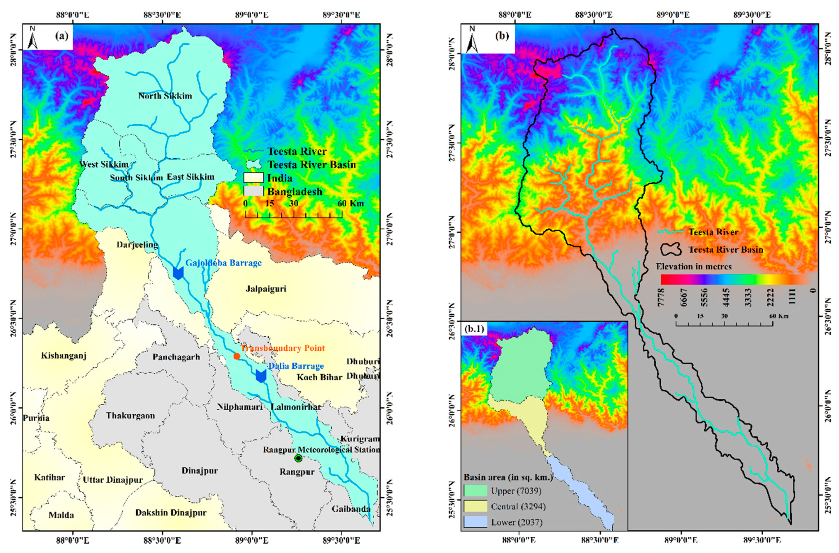
Figure 1. Map showing (a) geographical location of the Teesta river basin along with the administrative divisions, (b) elevation, and (b.1) area covered by the river basin.
Atmosphere 13 00941 g001
Figure 2. Description of the methodology followed in the study.
Atmosphere 13 00941 g002
Figure 3. Spatial distribution of trend (significant at 95% confidence level) and magnitude in the seasonal and annual series of Tmax during the observational and future period (tilted upward arrow denotes significant increasing trend and vice versa).
Atmosphere 13 00941 g003
Figure 4. Spatial distribution of trend (significant at 95% confidence level) and magnitude in the seasonal and annual series of Tmin during the observational and future period (tilted upward arrow denotes significant increasing trend and vice versa).
Atmosphere 13 00941 g004
Figure 5. Spatial distribution of trend (significant at 95% confidence level) and magnitude in the seasonal and annual series of precipitation during the observational and future period (tilted upward arrow denotes significant increasing trend and vice versa).
Atmosphere 13 00941 g005
Figure 6. Spatial distribution of trend (significant at 95% confidence level) and magnitude in the seasonal and annual series of potential evapotranspiration during the observational and future period (tilted upward arrow denotes significant increasing trend and vice versa).
Atmosphere 13 00941 g006
Figure 7. Spatial distribution of trend (significant at 95% confidence level) and magnitude in the seasonal and annual series of water availability during the observational and future period (tilted upward arrow denotes significant increasing trend and vice versa).
Atmosphere 13 00941 g007
Table 1. Salient features of the Teesta river basin.
Basin SectionCountryState/Division (District)Basin Area in km2Climatic Class by Köppen–GeigerShare of Water (%)Population Density/km2
Upper partIndiaSikkim (East, West, North, and South Sikkim)7039BWk a, BSk b, Dwc c, Dwb d, Cwb e5787
Central part West Bengal (Darjeeling, Jalpaiguri, Cooch Behar)3294Cwa f, Cwb e26525
Lower partBangladeshRangpur (Gaibandha, Kurigram, Lalmonirhat, Nilphamari, and Rangpur)2037Cwa f, Aw g171091
Entire basinIndia, Bangladesh-12,370-100369
a Arid desert cold; b arid steppe cold; c cold dry winter cold summer; d cold dry winter warm summer; e temperate dry winter hot summer; f temperate dry winter warm summer; g tropical savannah. Source: [19,20,21].
Publisher’s Note: MDPI stays neutral with regard to jurisdictional claims in published maps and institutional affiliations.

