Article

Modeling of Bi-Polar Leader Inception and Propagation from Flying Aircraft Prior to a Lightning Strike

Electrical Engineering Department, Indian Institute of Science, Bangalore 560012, India
*
Author to whom correspondence should be addressed.
Atmosphere 2022, 13(6), 943; https://doi.org/10.3390/atmos13060943
Submission received: 3 May 2022 / Revised: 28 May 2022 / Accepted: 6 June 2022 / Published: 9 June 2022

Abstract

:
Lightning is one of the major environmental threats to aircraft. The lightning strikes during flying are mostly attributed to aircraft-triggered lightning. The first step toward designing suitable protective measures against lightning is identifying the attachment locations. For this purpose, oversimplified approaches are currently employed, which do not represent the associated discharge phenomena. Therefore, in this work, a suitable model is developed for simulating the inception and propagation of bi-polar leader discharge from the aircraft. Modeling of leader discharges requires field computation around the aircraft, which is carried out employing the Surface Charge Simulation Method (SCSM) combined with sub-modeling, which ensures the best accuracy of field computations near nosecone, wingtips, etc. A DC10 aircraft model is considered for the simulation. Simulations are performed for different pairs of leader inception points on aircraft using the developed model. Subsequently, corresponding ambient fields required for stable bi-polar discharge from aircraft are determined. These values are in the range of measured ambient fields reported in the literature. In summary, the present work has come up with a suitable model for simulating the bi-polar leader inception and propagation from the flying aircraft. Using the same, a detailed quantitative description of the discharge phenomena from the aircraft is provided.

1. Introduction

Since the early age of aviation, lightning strikes have been proven to be hazardous to aircraft. It is estimated that on average, a commercial aircraft gets struck by lightning once in every 1000 flight hours, which is approximately equivalent to once in a year [1]. The effect of a lightning strike on aircraft spans from minor damages (i.e., burn marks on the skin, creation of holes, local deformation of parts, etc.) to complete destruction of aircraft (due to damage to fuel tanks, an explosion of the air–fuel mixture, destruction of internal circuitry, etc.). Hence, the threat caused by lightning needs serious consideration. Adding on to it, in modern aircraft, fiber-glass, carbon fiber, etc., materials are being increasingly employed due to their higher strength to mass ratio. However, due to their poor conductivity, the stroke current can lead to structural damage and higher field diffusion in the interior regions. In addition, extensive use of sensitive electronic equipment has further escalated the risk due to lightning strikes. According to National Oceanic and Atmospheric Administration, lightning strikes cost approximately two billion dollars for airline operators, excluding repair expenses [2]. Therefore, lightning protective measures have become an inextricable part of modern aircraft design.
A lightning strike on aircraft can occur in two possible ways. Bi-directional leaders can get initiated from aircraft in a high ambient field created by cloud and stepped leader. This type of aircraft-initiated lightning is responsible for almost 90 % of the recorded cases so far [3]. The other rare event is the aircraft intercepts a descending lightning leader from the cloud. Hence, considering the higher probability of the former type of attachment, this work will only be confined to aircraft-initiated lightning strikes.
Several in-flight measurement programs have provided insight into the phenomena associated with a lightning strike on aircraft. NASA’s Storm Hazard Program (F-106B aircraft, 1978–1986) [4,5,6], USAF/FAA Lighting Characterization program (CV-580 aircraft, 1984–1987) [7,8], ONERA/CEV Transall Program (C-160 aircraft, 1984, 1988) [9,10], and most recently the EXAEDRE project (Falcon 20 aircraft, 2016–2019, France) [11] are the major programs which were conducted to gather data on lightning strike. In all these programs, instrumented aircraft have been flown intentionally in and around the thundercloud to record the electric field and currents at selected locations preceding to and during the lighting strikes. Some recorded videos [10] have provided more clarity on the mechanisms involved in lightning attachment to aircraft.
Based on the descriptions provided by these research programs [4,7,9,11], and subsequently by several researchers [10,12], a schematic representation of the bi-polar leader discharge from a flying aircraft is shown in Figure 1. Under the influence of the lower negative charge center of the cloud and the associated negative descending leader, positive charges majorly appear on the top portion (indicated by the red plus sign) and the negative charges on the bottom part (indicated by the negative blue sign) of the aircraft (Figure 1a). The field due to the charge separated will compensate for the ambient field ( E c ) so as to ensure the equipotentiality of the aircraft. The distribution of these bi-polar charges depends on the relative orientation of aircraft with respect to the ambient field. Depending on the aircraft geometry, these charges distribute themselves on the aircraft. As a result, field intensification happens at the extremities like wing tips, vertical stabilizers, nosecones, etc. From these locations, corona discharges set in once the total electric field exceeds the critical value for corona inception (Figure 1b). If the spatial field strength is sufficiently high, the corona discharge gets converted to a streamer. The positive and negative streamers are shown as red and blue colored cone-shaped regions in Figure 1b respectively. In this particular example, for the purpose of illustration, it is assumed that the positive discharge is incepted from the tip of the vertical stabilizer and negative discharge from the nosecone of the aircraft. Subsequently, the streamers get converted to leaders, and the bi-polar leader discharge sets in from the aircraft (Figure 1c). Generally, the inception points of positive and negative leaders are called the Entry point and Exit point respectively (Figure 1c).
Most of the recorded incidents of lightning strikes on aircraft suggest that the inception of the positive leader occurs before the inception of the negative leader. Once the positive leader propagates a few tens of meters, the negative leader initiates from the location where the negative field intensification is maximum ([12]). In the schematic sketch (Figure 1c), the negative leader is shown to be incepted from the nosecone of the aircraft. Once the leaders with both the polarities appear, the bi-polar leader discharge continuously grows until the bridging occurs between the upward leader and descending stepped leader.
Depending on the lightning attachment points and resulting current distribution, the aircraft surface can be classified into different zones. This part of designing is called “Zoning” where the outer surface of aircraft is divided into well-defined regions (1A, 1B, 1C, 2A, 2B, 3 as suggested in [13]) depending on how they experience different phases of lightning stroke. This study in this paper only deals with identifying the initial attachments points on aircraft, which fall under Zone 1A and 1B.
Several methods for the zoning of aircraft have been developed in the last few decades. In 1989, British Aerospace (BAe) proposed a method of zoning of aircraft [14] based on the Rolling Sphere Method (RSM) [15] which is an empirical method based on the Electro-geometrical method (EGM) [16]. EGM, which was developed for lightning protection of transmission lines, was later modified to RSM for lightning protection of grounded objects. RSM is a well-recognized and widely used method for lightning protection of grounded objects. In RSM, a sphere with a radius of striking distance (calculated from prospective return stroke current) is rolled over the objects to determine the probable locations for lighting strike [15]. In 1999, the Society of Automotive Engineers (SAE) published a regulatory document, “ARP5414A” [13] regarding the zoning of an aircraft. In this standard, the approach involved in RSM for grounded objects has been extended for the zoning of aircraft. In the literature [13], apart from RSM, the similarity principle has been suggested where zoning was conducted based on zone data available from previously certified aircraft. This method is entirely qualitative and only applicable for aircraft with similar geometries. Field-based approaches for zoning and zoning based on laboratory testing on a scaled model of aircraft or isolated parts of aircraft have been mentioned in this literature [13] as well. In 2012, Lalande et al. proposed a probabilistic method of zoning of aircraft [17] based on previous methodologies (RSM, similarity principle, laboratory testing). These existing methods for zoning are highly simplified and do not include different aspects of long air gap breakdown. For a more accurate assessment, the inception and propagation of bi-directional leaders from aircraft need to be taken into account. None of these aforementioned methods have considered the discharge mechanisms involved in lightning attachment in detail. In view of the above, this work aims to develop a model for bi-polar discharge from aircraft, which will lead to the identification of lightning attachments points.
Experimental works have been reported in the literature on bi-polar discharge from floating objects in laboratory gaps. In 1995, Rizk came up with an analytical model [18] for the breakdown of long laboratory gaps (5, 8 m), including a floating conductor under applied switching impulse. Subsequently, in 1998, Castellani et al. also presented experimental data on discharge from a floating object placed in a 10.5 m long plane–plane gap [19,20]. Most recently, Jiachen Gao et al. [21] reported breakdown voltages of a gap of 2 m in the presence of floating rods and spheres.
The sequence of events associated with lightning initiation from aircraft is well established and widely accepted. However, due to the complexity involved in the discharge mechanism, literature on modeling of discharge from aircraft is rather difficult to find. Therefore, this work focuses on the development of a suitable macroscopic model for bi-polar discharge from aircraft prior to aircraft-triggered lightning strikes. Discharge from a flying aircraft involves both positive and negative leader discharges. Invariably, models for lightning attachment are developed based on laboratory findings. Therefore, detailed literature surveys on positive and negative leader discharges in long air gaps are carried out.

2. Modeling of Bi-Polar Discharge from Aircraft

2.1. Modeling of Positive Leader Discharge

Positive discharge in long air gaps starts with the initiation of a positive corona followed by positive streamer bursts with a common stem. If the existing ambient field is increasing or sufficiently high, the streamer grows, and the corresponding charge flow causes heating of the stem to more than 1500 K. Due to this thermalization of the stem, it gets converted to a leader [22]. Several such intermittent leaders emerge and vanish before a stable leader propagation gets established. This stable leader propagates continuously with a positive streamer zone ahead of it.
Over the years, several models for positive leader discharge have been proposed. Hutzler’s model for leader propagation [23], the Critical radius criterion [24,25], Critical streamer length criterion [26,27], empirical model [28,29], and thermo-hydrodynamical model [22] are the few mentions. In 2006, using the findings of Gallimberti et al. [22,30], Becerra and Cooray proposed a physical model [31] called the self consistent leader inception model (SLIM). This model was validated for leader discharges in laboratory gaps [31], connecting leader inception from grounded objects [31] and for rocket triggered lightning [32] as well. The SLIM needs significant computational resources. To reduce that, a simplified model is also suggested in [31]. This simplified method was successfully implemented on grounded structures [33,34]. For inception and propagation of positive connecting leader from aircraft, this simplified model [31] is considered.
In Figure 2, a schematic of positive leader discharge from an electrode is shown (at the top) along with a corresponding distance–voltage diagram (at the bottom). The distance–voltage diagram includes the potential distributions along the discharge axis at different instants of discharge growth. The blue color curve ( P b a c k ) in distance–voltage diagram (Figure 2) represents the background potential distribution. Once, the streamer appears, it is represented with a straight line ( P ( 0 ) ) with a slope set to the positive streamer gradient [31]. Each green and red color curve ( P ( i ) for i t h leader increment) represents the potential distribution for leader length at one instant, where the red part corresponds to the positive streamer. The leader itself is represented by a straight line (green color with the slope set to the leader gradient.
The steps involve in this model ([31]) are explained with the reference of Figure 2.
  • Adding up ambient potential and reaction potential due to induced charges on aircraft, total potential distribution ( P b a c k in Figure 2) is obtained.
  • A straight line with a slope of 450 kV/m is considered as streamer section (such as P ( 0 ) in Figure 2). Streamer charge is computed from the area between background potential distribution and modified potential distribution (Equation (1)) [30,31].
    Q s t r = K Q 0 l s t ( 1 ) ( P b a c k P ( 0 ) ) d x
    where x is the distance along the discharge axis. K Q is the geometrical factor whose value is taken as 4 × 10 11 C/V·m.
  • If Q s t r 1 μ C , positive discharge starts with an initial length of 5 cm. The corresponding potential drop along the leader length is calculated using Rizk’s equation [31],
    V l d r o p ( i ) = l L ( i ) E + x 0 E ln [ E s t r E E s t r E E e l L ( i ) x 0 ]
    where l L ( i ) is the leader length at i t h step, E s t r is gradient of positive streamer, E = 30 kV/m is the final quasi-stationary leader gradient, and x 0 = 0.75 m is the time constant.
  • In subsequent steps, the incremental streamer charge ( Q s t r ( i ) ) is again calculated from the area between two consecutive potential distributions. Subsequently, the incremental leader length is evaluated.
    Q s t r ( i ) = K Q l L ( i 2 ) l s t ( i 1 ) ( P ( i 1 ) P ( i 2 ) ) d x
    l L ( i ) = Q s t r ( i ) q L
    where P ( i ) is the potential distribution at t t h instant in presence of leader and streamer both (Figure 2). q L = 65 μ C/m, is the charge per unit length of positive leader [31].
  • The modified leader length at i t h instant is calculated as l L ( i ) = l L ( i ) + l L ( i ) .
A more elaborated explanation of different aspects of this positive leader model is available in [31].

2.2. Modeling of Negative Leader Discharge

Unlike positive leader discharges, negative leader discharges are more complicated physical phenomena. The first phase of negative discharge is the formation of a negative corona if the field value at the electrode exceeds a critical level. Once the corona attains its critical volume, i.e., contains a critical amount of negative charges, a space stem appears at the tip of the discharge [19,35]. This space stem initiates bi-directional streamers called a pilot system involving a positive streamer towards the electrode and a negative streamer ahead of the discharge, as shown in Figure 3(II). Injection of these streamer charges heats up the space stem and converts it into bi-directional space leaders. When the positive space leader reaches the primary negative leader tip, all the streamer charges flow to the electrode through the discharge channel resulting in a sudden elongation of the main negative leader [35]. This phase is observed as a highly illuminated channel in recordings of laboratory discharge [35]. Again, a negative streamer is formed ahead of the newly formed extension of the negative leader (Figure 3(IV)), followed by the formation of a space stem. These inter-step processes keep on repeating, which results in step-wise elongation of negative discharge.
Despite having substantial experimental data (Les Renadieres [35], Castellani et al. [19,20]), research on the physical model of negative leader discharge is limited. In 1994, Bechhiega et al. [36] developed a theoretical model for negative leader discharge. Subsequently, Mazur et al. [37], L. Arevalo, and Cooray [38] came up with physical models for negative discharges. The RLC linear circuit model for negative discharge was presented by Rakotonandrasana et al. [39] and most recently, in 2019 Zixin Guo, Rakov et al. [40] proposed a simplified model for negative leader propagation. Because of ease of implementation and requirement of less computational resources, this model [40] is considered for negative leader inception and propagation from aircraft. This model is validated in [40] for different laboratory gap discharges.
For the negative leader discharge, a different distance–voltage diagram can be drawn as shown in Figure 4. The background potential distribution prior to negative discharge is shown as V b a c k ( 0 ) (black curve). Once, the primary negative streamer appears, it is shown with a straight line (blue line, P ( 0 ) ) with a slope set to the negative streamer gradient. The intersection between V b a c k ( 0 ) and P ( 0 ) provides the axial extension of the negative streamer and it is also the position at which the space stem (shown with a black dot) appears. The potential distributions for different space leaders lengths are labeled as P ( 0 ) , P ( 1 ) , P ( 2 ) , P ( 3 ) . Positive (red line) and negative space streamers (blue line) are represented with straight lines with slope set to their respective streamer gradient. The space leaders are shown with horizontal lines (dashed), while the primary negative leader is shown with a black (dashed) line in the distance–voltage diagram (Figure 4).
The steps involved in this model [40] can be briefly stated with the reference of distance–voltage diagram shown in Figure 4 as follows,
  • Like a positive streamer [31], negative streamer charge is also calculated from the area between background potential ( V b a c k ) and potential distribution modified by negative streamer ( P ( 0 ) , Figure 3) which is represented as a straight line with a slope of 750 kV/m in Figure 4.
    Q s t r = K Q · 0 l s s ( V b a c k ( 0 ) P ( 0 ) ) d x
  • If Q s t r 0.8 μ C [19], the pilot system starts from the boundary of the negative streamer followed by inception of space leaders.
  • Space leaders are represented with horizontal lines (zero leader gradient [40]) in Figure 4. Corresponding space streamer charges ( Δ Q s t r p ( i ) and Δ Q s t r n ( i ) ) are computed from the area between the potential distributions as shown in Equation (6). Subsequently, the incremental space leader lengths ( Δ l P S L ( i ) and Δ l N S L ( i ) ) are calculated from the incremental space streamer charges (Equation (6)).
    Δ Q s t r p ( i ) = K Q · l L ( i 1 ) l p s l ( i 1 ) ( P ( i 2 ) P ( i 1 ) ) d x Δ Q s t r n ( i ) = K Q · l n s l ( i 1 ) l n s t r ( i 1 ) ( P ( i 2 ) P ( i 1 ) ) d x Δ l P S L ( i ) = Δ Q s t r p ( i ) q P S L ; Δ l N S L ( i ) = Δ Q s t r n ( i ) q N S L
    where P ( i ) is the potentil distribution along discharge axis at i t h instant. q P S L = 53.1 μ C/m, q N S L = 166.7 μ C/m [40] are the charge per unit length for positive and negative space leaders respectively.
  • The space leader length are update by adding the incremental leader lengths.
    l P S L ( i ) = l P S L ( i 1 ) + Δ l P S L ( i ) ; l N S L ( i ) = l N S L ( i 1 ) + Δ l N S L ( i ) ;
  • When the positive space leader tip reaches the primary negative leader i.e., l L ( i ) + l e n g t h p s l ( i ) l s s (Figure 4) the length of the negative leader jumps suddenly, and a stepping process is completed. The corresponding negative leader length is calculated as,
    l L ( i + 1 ) = l L ( i ) + l P S L ( i ) + l N S L ( i )
  • Again, these steps are followed for new extension of main negative leader.

2.3. Electric Field Computation

As explained in previous Sections (Section 2.1 and Section 2.2), modeling leader inception and propagation requires computation of the field around the aircraft. Because of the involvement of complex geometries, an analytical solution is not feasible. Therefore, an appropriate numerical computational methodology must be chosen for field computation.
The electric field distribution during the attachment can be considered as quasi-static because of the negligible contribution from the time-varying magnetic field. Hence, Poisson’s equation ( 2 ϕ = ρ / ϵ ) needs to be solved in space where the charge density at the RHS arises due to corona and streamer charges. As this problem is an open geometry problem, boundary-based methods appear to be more appropriate over domain-based methods. Hence, considering applicability and accuracy, the surface charge simulation method (SCSM) [41,42] is employed for computation of field and potential.
In the SCSM, the surface of the geometry is divided into surface elements. The point collocation scheme of the SCSM is employed where the residues ( R i ), i.e., the difference between computed potential ( ϕ ˜ ) and known potential ( ϕ k n o w n ) is forced to zero at the center of each surface element.
R i = ( ϕ ˜ i ϕ k n o w n i ) = 0 ; f o r , i = 1 t o n p ,
where n p is the number of surface elements. The condition of Equation (9) provides a set of linear equations by solving which the unknown charge densities on surface elements can be obtained. Steps involved in field computation using the SCSM are described in [41,43].

2.3.1. Salient Features of Bi-Polar Leader Discharge from Aircraft

Aircraft skin is considered to be conducting. For both metallic and aircraft in composite elements, it is worth recalling that the composite parts are covered with aluminum/copper mesh to provide conducting path for the lightning current. Therefore, a cruising aircraft acts as a floating conductor whose potential is not known beforehand. Hence, another condition of zero net charges on aircraft is brought into the potential co-efficient matrix, and then it is solved for both the unknown aircraft potential and surface charges. Details of this method are available in [41,42].
Unlike grounded objects or excited laboratory electrodes, the potential of the aircraft changes with increments in connecting leader lengths and also with the change in the ambient field. Hence, after each stage of leader propagation, the modified potential distribution needs to be re-calculated, which requires modeling of connecting leaders. Connecting leaders (of either polarity) are modeled using several segments with cylindrical charge distribution whose density is considered to be varying linearly within each segment. Boundary conditions are imposed on each leader segment based on corresponding leader gradients as suggested in the adopted models for the positive [31] and negative leader [40]. For every new leader segment, one row and one column are appended to the main potential coefficient matrix. This augmented matrix forms the new SCSM potential co-efficient matrix by solving which modified charge distribution due to connecting leaders, and corresponding aircraft potential is obtained.
For this work, a commercial aircraft model McDonnell Douglas DC-10 (dimensions: length—55.55 m, wingspan—47.35 m, height—17.86 m) was downloaded from [44]. It should be noted that the radome of the actual aircraft is built with non-metallic materials to provide transparency to the antenna communication. For protection of the radome, several segmented metallic diverter strips are installed on it. Due to the unavailability of the number and dimensions of the diverter strips for this particular aircraft model, the radome portion is also considered as a conducting structure like the rest of the aircraft. The outer surface of this aircraft model is discretized into 11,000 triangular surface elements using MeshLab software. This results in the formation of an 11 k × 11 k co-efficient matrix in the SCSM.
The potential distribution around the DC10 aircraft, cruising at the altitude of 500 m from the ground under a uniform ambient field of 50 kV/m (in a vertically upward direction) is illustrated in Figure 5.

2.3.2. Accurate Evaluation of Local Field Using Sub-Modeling

The total electric field gets significantly enhanced at sharp edges and corners of aircraft like nose cones, vertical stabilizers, wing tips, etc., which can initiate connecting leaders. The radius of curvature at edges and corners is typically in the order of a few centimeters, and in some places, it is even less. Therefore, local field intensification caused by these regions gets weakened within a meter. For precise modeling of these highly localized perturbations, Sub-modeling [43] is employed. In this method, a critical region of original geometry is remodeled, and an artificial boundary is constructed around it. The potential of this boundary is evaluated from the solution of the original problem. All the field computations inside the sub-model are performed using the charge simulation method (CSM) [45] by considering the imposed boundary conditions. The sub-model is employed at the very initial stage of discharge, where the critical regions majorly govern the field distribution. Once the discharge propagates by significant length (i.e., one meter of leader length), the sub-modeling is removed, and subsequent calculations are performed using the original discretization.
A sub-model with a shape of truncated ellipsoid (major axis—3–4 m and minor axes—1–2 m) is employed around the critical regions (Figure 6). The maximum error in computed potential on the sub-model is kept below 0.1 % which ensures sufficiently accurate local modeling of edges and corners.
A 3.5 m long axis is considered in normal direction from the tip of vertical stabilizer where sub-modeling is also employed. Potential distributions along the axis evaluated using both the original discretization and sub-model are presented in Figure 7.
From Figure 7, it can be seen that the sub-model provides a more detailed distribution of potential as compared to the original geometry.

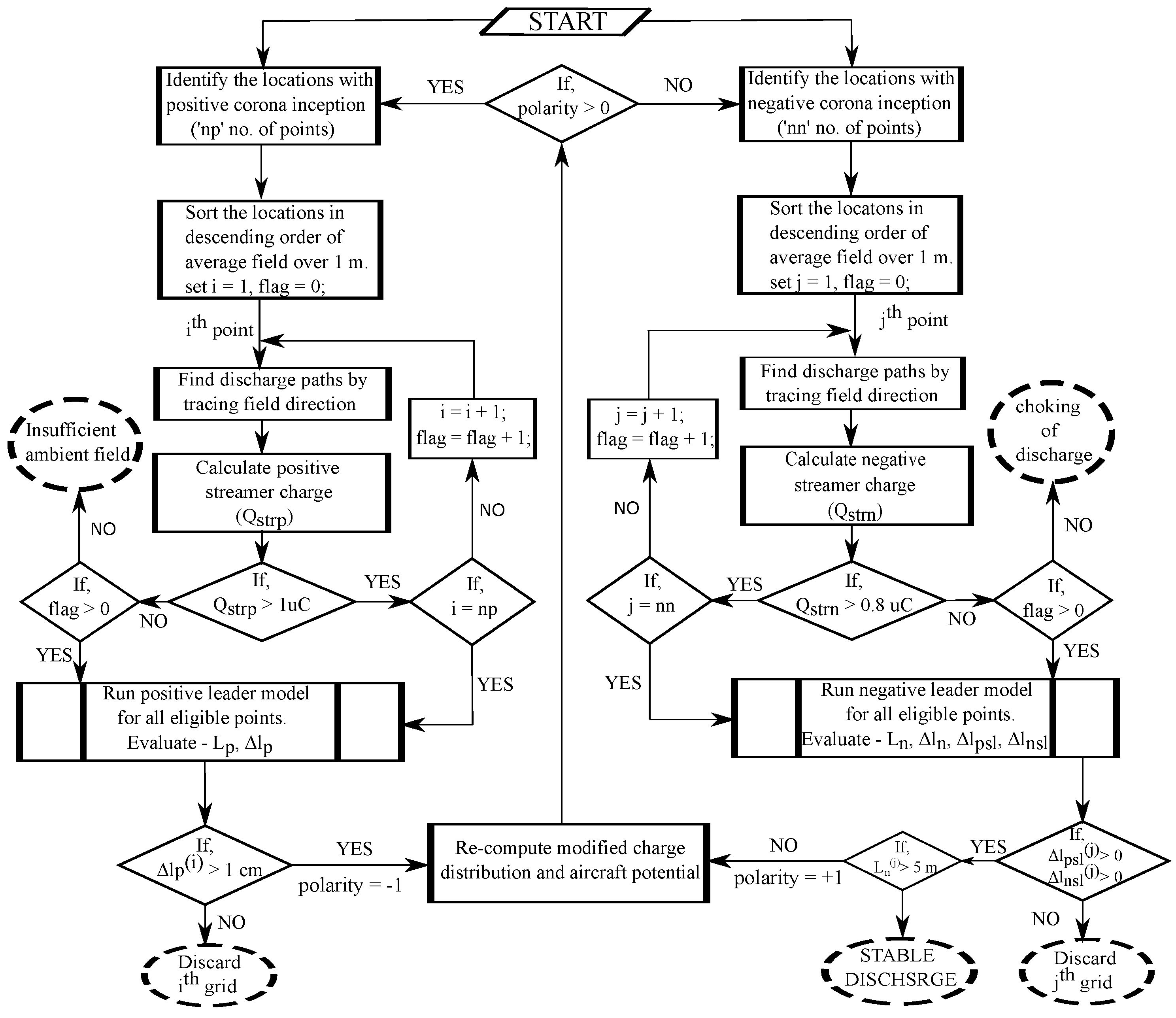
2.4. Steps Involved in Simulation

According to the existing literature [25,26,29,31], for grounded objects, 2–5 m length of positive connecting leader ensures a stable propagation. However, for aircraft, it is seen from the in-flight measurements [4,7,9] that at least 10 m of positive leader length is required for the inception of negative leader from other extremities. Therefore, the simulation needs to be performed until both the connecting leaders attain significant lengths. Sequences of steps involved in the simulation of bi-directional leader discharge are,
  • The simulation begins with the identification of the locations on the aircraft where the condition for positive [31] or negative [40] corona inception is reached. Once the locations of corona onset are identified, criteria for the inception of the initial leader section are checked.
  • From the locations of leader inception, discharge paths are determined by tracing the direction of the electric field. Initial leader extensions are considered along the corresponding discharge axis.
  • Modified potential distribution is computed, including the newly formed connecting leader segments (Section 2.3).
  • Subsequently, at the locations of leader inception, corresponding incremental positive and negative leader lengths are obtained.
  • If, at any location, the incremental leader length decreases in a few consecutive steps and becomes less than 5 mm , it is considered an unsuccessful leader inception. Further computation at that location is terminated.
  • For the other locations where significant leader increment is obtained, steps 3, 4, and 5 are performed until a stable bi-polar discharge from the aircraft gets established.
Details of the simulation steps are shown in a flowchart in Figure 8.
For both the field computation using the SCSM and subsequent leader inception and propagation, codes are written in MATLAB-R2017b. The simulation time is typically 24–30 h on a computer with Intel Core i 5 8400 C P U @ 2.80 GHz and 64 GB RAM with Ubuntu operating system.

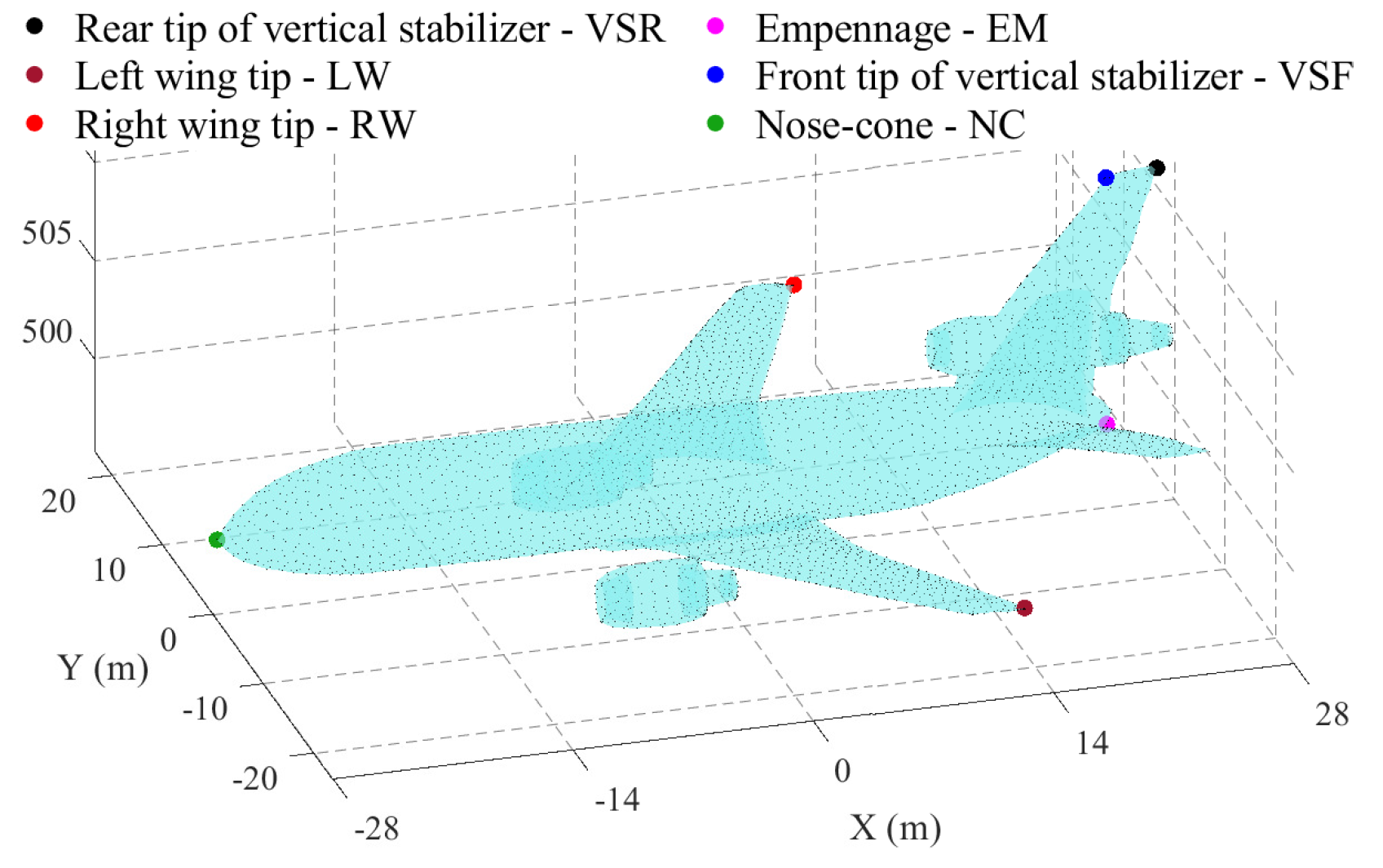
3. Simulation Results for DC-10 Aircraft

The locations of connecting leader inception points depend on the aircraft’s orientation relative to the ambient field. There are specific ranges of permissible pitch, yaw, and roll angles. At the same time, the ambient field due to the lightning leader could be in many directions. For understanding the different steps involved in the inception and propagation of the bi-polar leaders, certain variables need to be fixed. With the intention of clearly identifying the steps, the aircraft is considered to be in a cruising position. However, the direction of the ambient field is not constrained. Kindly note that the model developed is not limited to any particular aircraft orientation.
Bi-polar leader inception happens due to distortion of the ambient field around the aircraft. The ambient field might be caused by cloud charges, approaching leaders, or a combination of these. As a first step towards modeling the inception and propagation of the bi-polar leaders from the aircraft, instead of any specific source, static and uniform ambient field ( E 0 ) distribution is considered. This would help in segregating the influence of different participating factors. Inception points for positive and negative leaders depend on the relative orientation of the ambient field with respect to the aircraft. Depending on the local field intensification for different directions of the ambient field, some probable leader inception locations are marked on the aircraft (Figure 9). In the same, the aircraft extremities are named with some letters which will be used in the following discussion to denote the corresponding location. Subsequently, simulation is carried out as per the details provided in Section 2.4.
In this study, four different events (Cases-A, B, C, and D in Table 1 of bi-polar leader inception from a aircraft cruising (roll, pitch, and yaw angles are 0, as shown Figure 9) at an altitude of 500 m are considered. The ambient field directions (refer to Table 1) are chosen in such a way that distinct pair of inception points (marked in Figure 9) is obtained. For Case-A, equipotentials on a bisecting x z plane around the inception locations, at different instants are shown in Figure 10. This clearly indicates how the background field gets distorted during the propagation of connecting leaders from aircraft.
Propagation of connecting leaders and the corresponding change in aircraft potential for all the cases (Cases-A, B, C, and D) are shown in Figure 11. Results for four different pairs of inception locations are provided in this figure. The figures in the top row i.e., Figure 11a–d display the orientation of the aircraft relative to the ambient field considered and corresponding propagation paths of the bi-polar leader of the aircraft in different cases. The figures in the bottom row i.e., Figure 11e–h show the variation in connecting leader lengths (blue and red curves) and corresponding variation in aircraft potential (black curve). In these figures, the left y-axis corresponds to the length of connecting leaders while the y-axis at the right represents the percentage change of aircraft potential ( % Δ V a i r c r a f t ). It should be noted that the time axis shown in Figure 11, is a pseudo time scale that is determined in such a way that the velocity of the positive connecting leader throughout the simulation period remains within the range of 2 × 10 4 to 10 6 m/s. The percentage changes in aircraft potential ( % Δ V a i r c r a f t ) in Figure 11 are calculated with respect to the magnitude of aircraft potential just prior to leader initiation ( V i n i t i a l ) i.e., % Δ V a i r c r a f t = V a i r c r a f t V i n i t i a l | V i n i t i a l | × 100 . Where V a i r c r a f t is the potential of aircraft at any instant after leader initiation.
It is worth mentioning that aircraft potential is always negative as the ambient field is considered to be negative (directed upward). Hence, in the subsequent explanations, an increase in aircraft potential refers to a more negative potential of aircraft and vice versa.

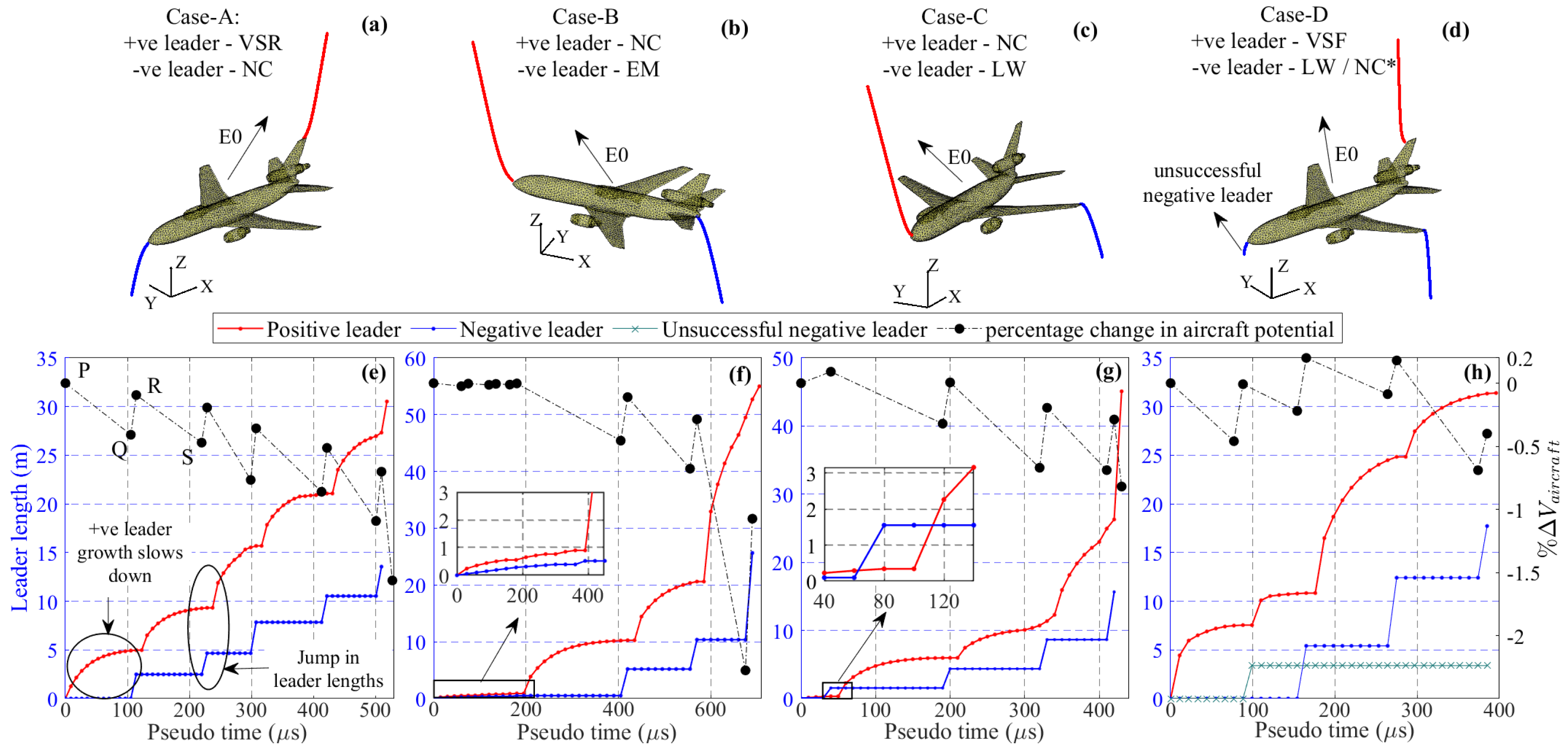
Analysis of Propagation of Connecting Leaders

Case-A in Figure 11 is considered as a reference event for describing the phenomena involved in bi-directional leader propagation. In this case, the positive leader incepts from the tip of the vertical stabilizer prior to the negative leader from the nosecone (Figure 11a).
As the positive leader elongates, it deposits negative charges on the aircraft causing aircraft potential to increase, which is indicated as P to Q in Figure 11e. This slows down the growth of the positive leader (encircled in Figure 11e) and, on the other hand, facilitates the inception of the negative leader from the nosecone. Once the negative leader appears, aircraft potential decreases (Q to R in Figure 11e) due to the deposition of positive charge, which causes a rapid increase in positive leader length. As the positive leader propagates, the aircraft potential again increases (R to S in Figure 11e) and thereby slowing down its growth until stepping occurs at the negative leader discharge at the nosecone. This cycle keeps on repeating in subsequent propagations.
It is worth mentioning that if during the retarding phase (P-Q or R-S in Figure 11e) of positive leader progression, the negative leader does not incept, the positive discharge would have been choked, resulting in unsuccessful leader inception from aircraft. Hence, stable uni-polar discharge from a cruising aircraft is non-viable as it always needs support from the discharge of opposite polarity.
The critical field required for positive leader inception and propagation is less compared to the negative leader [22]. Therefore, in most of the recorded events of lightning strikes to aircraft [46], positive leader inceptions were reported to occur prior to the negative leader. This is also observed in Cases-A, B, and D (Figure 11). However, the local field intensification around the inception location strongly influences the inception and the initial phase of leader propagation from aircraft. Therefore, for some specific directions of the ambient field, the negative leader might get incepted earlier. This phenomenon is observed in Case-C (Figure 11g) where the first significant increment occurs in negative leader length. A smaller radius of curvature at the wing tip than the nosecone provides an earlier elongation of the negative leader. Once the leader grows, the effect of the local radius of curvature gets weaker, and the positive leader propagates faster than the negative leader.
If sufficient field intensifications occur at multiple locations of aircraft, multiple positive or negative leader inceptions can happen. Such phenomenon is observed in Case-D where multiple negative leaders (nosecone and wing tip) incept at different instants of discharge (Figure 11d). First, the positive leader starts propagating from vertical stabilizer (VSF, Figure 9). Then a negative leader incepts from the nosecone, followed by the inception of another negative leader from the wing tip (Figure 11h). The direction of the ambient field (Table 1) is more aligned to the negative leader from the wing tip than the nosecone resulting in stable propagation from the wing tip. On the other hand, the negative leader from the nosecone gets choked off after 3.5 m of propagation due to the lack of spatial field strength.

4. Ambient Electric Field Required for Stable Bi-Polar Discharge from Aircraft

After the inception of bi-polar leaders from the aircraft, their growths depend on the net field at the tips of the leaders. Generally, the ambient field required for the inception is higher than the ambient field required for propagation. Further, the ambient field created by the cloud and descending leader is maintained for large spatial extensions and thereby ensuring continuous growth. Based on the simulation results on DC-10 aircraft, it is seen that typically 10–20 m of positive and negative leader propagation is required to ensure a stable bi-polar discharge from aircraft. Simulations are carried out following the steps described in Section 2.4. Minimum ambient fields ( E 0 ) obtained for stable bi-polar leader discharge from DC10 aircraft are given in Table 1. It includes several pairs of leader inception locations as shown in Figure 11. Corresponding ambient potential differences ( Δ V p n ) between the pair of leader inception locations are also mentioned in Table 1. It can be seen that the magnitude of E 0 varies significantly for different pairs of leader inception points. These higher ambient field values mentioned in Table 1 might not be established by the cloud charges alone. However, in the presence of an approaching descending leader, the ambient field can reach that range.
The ambient field values reported in Table 1 are for cruising aircraft. However, during takeoff and landing, due to changes in aircraft orientation, the ambient field required for stable bi-polar leader inception will differ from the case of cruising aircraft. For instance, ambient fields evaluated for three different pitch angles (i.e., the angle between the axis along the fuselage and horizontal axis) corresponding to landing and takeoff are shown in Table 2. The directions of the ambient field are considered the same as Case-A (for landing) and Case-B (for takeoff). It can be seen that for a fixed direction of the ambient field, aircraft with a higher pitch angle require less ambient field for the inception of stable bi-polar leader discharge. However, the component of the ambient field along the positive and negative leader inception points increases with pitch angle. As a result, the ambient potential difference ( Δ V p n ) between the leader inception points increases.
In Table 3, ambient field values measured before the lightning strike on aircraft in different research campaigns [7,9,11] and the dimensions of aircraft used in these campaigns are provided.
The DC-10 aircraft model, considered for this study, is larger than these aircraft. The geometry of aircraft strongly influences the bi-polar discharge from aircraft [12,47]. Moreover, during the measurement, the orientation of the aircraft, and leader inception locations are also not explicitly mentioned in the literature. Even though more details are required for a precise comparison, it is worth noting that the ambient field at the stable bi-polar leader inception, as predicted by the model, is in the close range of the measured ambient fields corrected to STP ( E S T P ).

5. Discussion

This work develops the model for bi-polar leader inception and propagation from aircraft based on available positive and negative leader models. Different discharge parameters used in the simulation exercises reported in Section 3 and Section 4, correspond to STP (20 C temperature, 1 atm pressure). However, the atmospheric conditions change with altitude. Further, the movement of the aircraft causes a very localized change in ambient conditions like air density and pressure around the aircraft. All these influence the inception and propagation of connecting leaders from aircraft. Therefore, this section aims to provide a pertinent review of these factors.

5.1. Atmospheric Conditions

Atmospheric conditions such as relative air density and humidity have a strong impact on the leader discharges [22]. Commercial aircraft are usually not flown inside a thundercloud. Hence, they get struck by cloud-to-ground lightning, typically at an altitude of ≤6 km. Within this range of altitude, the atmospheric conditions vary significantly. All the data presented in Table 1 and Table 2 are based on streamer and leader parameters suggested at STP. To obtain the results corresponding to flying conditions, atmospheric factors must be brought in. Streamer gradients (determine the streamer charges) and charge per unit length of leader ( q l , related to the rate of energy input at the head of a leader, decides leader speed) are the two most impactful parameters for leader discharge. Streamer gradients have a strong correlation with air density and humidity, which is readily available in [48,49]. On the other hand, the charge per unit length of a leader ( q l ) varies significantly with water content in the air [22], but its relationship to air density is not clearly reported in the literature. Further, the local humidity at flying altitude is difficult to anticipate as it strongly depends on the vicinity of a thundercloud. Hence, the same q l values ([31,40]), suggested for discharges at standard conditions are used in subsequent computations. So, only including air density correction for streamer gradients, minimum ambient field ( E 0 ) for stable bi-polar discharge for Case-A (Figure 11) are recomputed for six different altitudes (Table 4). Relative air densities at different altitudes are obtained from the International Standard Atmosphere (ISA, [50]), and corresponding streamer gradients are calculated as suggested by the authors of [49] keeping the absolute humidity constant at 5 gm/m 3 . The first row of Table 4 corresponds to streamer gradients at STP. As compared to the critical field provided in Table 1, a significant reduction (4–40%) can be observed in Table 4 for altitude of ≤6 km.

5.2. Aircraft Speed

For most commercial aircraft, takeoff and landing speeds remain in the range of 66–80 m/s while the cruising speed could be as high as 246–250 m/s. Here, two aspects need consideration. At one of the attachment points, the discharge has to elongate so it has to be connected with the aircraft. At the other end, the connecting leader sweeping on the surface would tend to modify the local field disturbance caused by the aircraft. As reported in [12], the measured velocity of the upward positive leader from rocket-triggered lightning is between 2 × 10 4 to 10 6 m/s. Considering this velocity range, it will take approximately 500 μ s to simulate a few tens of meters of connecting leaders. Based on the aforementioned aircraft velocity and simulation time, the shifting distance (250 m/s × 500 μ s =12.5 cm) can be found to be less than a few tens of centimeters, whose effect can be considered negligible.
Due to the movement of the aircraft and relative airflow, variation of local air pressure and formation of vortices (usually trail from wing tips) occur around the extremities of a flying aircraft. Typically, the local pressure tends to increase around the leading extremities like the nosecone while it decreases at the trailing extremities like the wing tip, empennage, etc. These localized variations of pressure, and air density in the vicinity of probable leader inception locations might influence the inception of connecting leaders from aircraft. However, no efforts could be made in this work in that direction.

6. Summary

Noting that more than 90 % of the strike to the aircraft is due to the aircraft-initiated lightning, the present work, based on the works on impulse breakdown of long air gaps, has constructed a model for simulating the inception and propagation of the bi-polar leaders from the aircraft. It involves a detailed calculation of the associated electric field by employing the surface charge simulation method (SCSM) and sub-modeling. The inception and growth of the leaders are based on computationally efficient models. For the numerical simulation, the model of a DC-10 aircraft, which is readily available in an online source, is considered.
The simulation results indicate that under the action of a negative leader and the negative charge center in the cloud, a positive upward leader usually appears first (in most of the cases), which is followed by a negative downward leader.
It is shown that stable unipolar leader propagation is not possible without the support of an opposite polarity leader from the other side of the aircraft.
The minimum ambient field required for stable inception of bi-polar leaders from aircraft is strongly dependent on the orientation of the aircraft relative to the direction of the ambient field. Variation of air density and humidity with the flying altitude strongly impacts the bi-polar leader discharge from the aircraft. The higher flying altitude favors the initiation and propagation of bi-polar discharge from aircraft.
This work finds its application in two places. Firstly, it supports modeling the leader phase of the cloud-to-ground lightning involving an aircraft and quantifies the associated phenomena.
Secondly, it finds a serious application in the zoning of the aircraft for lightning protection. Identifying the initial attachment points (i.e., Zone-1A) of the aircraft is the first step for aircraft zoning. As most of the lightning strikes are dominated by the connecting leaders from the aircraft, the bi-polar discharge model proposed here is employed to identify Zone-1A. Unlike the usually employed and very conservative approaches for the identification of Zone-1A, a better quantification approach is presented.
In this work, some initial attachment points are identified on the aircraft which shows that Zone-1A is more limited than what is predicted by the rolling sphere method (which is a widely followed method for zoning) and hence provides a means for optimized design of the lightning protective measures.

Author Contributions

The problem has been conceptualized by U.K. (Udaya Kumar) and S.D. (Sayantan Das); Methodology, S.D.; The SCSM program for field computation was developed by U.K. and the programs for bi-polar leader discharges from aircraft were developed by S.D.; Validation, S.D.; Formal analysis, S.D.; Investigation, S.D. and U.K.; Resources, U.K.; Data curation, SD.; Writing—original draft preparation, S.D. and U.K.; Writing—review and editing, S.D. and U.K.; Visualization, S.D.; Supervision, U.K. All authors have read and agreed to the published version of the manuscript.

Funding

This research received no external funding.

Institutional Review Board Statement

Not applicable.

Informed Consent Statement

Not applicable.

Data Availability Statement

Not applicable.

Conflicts of Interest

The authors declare no conflict of interest.

References

  1. Fisher, F.A.; Plumer, J.A. Lightning Protection for Aircraft; National Aeronautics and Space Administration, Scientific and Technical Information Office: Huntsville, AL, USA, 1980.
  2. Golding, W.L. Lightning strikes on commercial aircraft: How the airlines are coping. J. Aviat. Educ. Res. 2005, 15, 7. [Google Scholar] [CrossRef]
  3. Lalande, P.; Bondiou-Clergerie, A.; Laroche, P. Analysis of Available In-Flight Measurements of Lightning Strikes to Aircraft; Technical Report; SAE Technical Paper; International Conference on Lightning and Static Electric: Onera, France, 1999. [Google Scholar]
  4. Fisher, B.; Plumer, J. Lightning attachment patterns and flight conditions experienced by the NASA F-106B airplane from 1980 to 1983. In Proceedings of the 22nd Aerospace Sciences Meeting, Reno, NV, USA, 9–12 January 1984; p. 466. [Google Scholar]
  5. Thomas, M. Direct strike lightning measurement system. In Proceedings of the 1st Flight Test Conference, Tokyo, Japan, 12–14 January 1981; p. 2513. [Google Scholar]
  6. Pitts, F.L. Electromagnetic measurement of lightning strikes to aircraft. J. Aircr. 1982, 19, 246–250. [Google Scholar] [CrossRef]
  7. Burket, H.D.; Walko, L.C.; Reazer, J.S.; Serrano, A.V. In-Flight Lightning Characterization Program on a CV-580 Aircraft; Technical Report, Report No. AFWAL-TR-88-3024; Air Force Wright Aeronautical Labs Wright-Patterson Afb Oh Flight Dynamics Lab: Wright-Patterson, OH, USA, 1988.
  8. Rustan, P., Jr. The lightning threat to aerospace vehicles. J. Aircr. 1986, 23, 62–67. [Google Scholar] [CrossRef]
  9. Laroche, P.; Dill, M.; Gayet, J.; Friedlander, M. In-flight thunderstorm environmental measurements during the Landes 84 campaign. Onera TP 1985, 1985, 9. [Google Scholar]
  10. Moreau, J.P.; Alliot, J.C.; Mazur, V. Aircraft lightning initiation and interception from in situ electric measurements and fast video observations. J. Geophys. Res. Atmos. 1992, 97, 15903–15912. [Google Scholar] [CrossRef]
  11. Buguet, M.; Lalande, P.; Laroche, P.; Blanchet, P.; Bouchard, A.; Chazottes, A. Thundercloud electrostatic field measurements during the inflight EXAEDRE campaign and during lightning strike to the aircraft. Atmosphere 2021, 12, 1645. [Google Scholar] [CrossRef]
  12. Mazur, V. A physical model of lightning initiation on aircraft in thunderstorms. J. Geophys. Res. Atmos. 1989, 94, 3326–3340. [Google Scholar] [CrossRef]
  13. Group, S.I. Aircraft Lightning Zoning, ARP 5414. In Aerospace Recommended Practice; Revision A; SAE: Warrendale, PA, USA, 1999. [Google Scholar]
  14. Jones, C. The Rolling Sphere As a Maximum Stress Predictor for Lightning Attachment and Current Transfer; International Aerospace and Ground Conference on lightning and Statis Electricity: Bath, UK, 1989. [Google Scholar]
  15. Lee, R.H. Protection zone for buildings against lighning strokes using transmission line protection practice. IEEE Trans. Ind. Appl. 1978, 6, 465–469. [Google Scholar] [CrossRef]
  16. Armstrong, H.; Whitehead, E.R. Field and analytical studies of transmission line shielding. IEEE Trans. Power Appar. Syst. 1968, 1, 270–281. [Google Scholar] [CrossRef]
  17. Lalande, P.; Delannoy, A. Numerical Methods for Zoning Computation; AerospaceLab: Mont-Saint-Guibert, Belgium, 2012; pp. 1–10. [Google Scholar]
  18. Rizk, F.A. Effect of floating conducting objects on critical switching impulse breakdown of air insulation. IEEE Trans. Power Deliv. 1995, 10, 1360–1370. [Google Scholar] [CrossRef]
  19. Castellani, A.; Bondiou-Clergerie, A.; Lalande, P.; Bonamy, A.; Gallimberti, I. Laboratory study of the bi-leader process from an electrically floating conductor. I. General results. IEE Proc.-Sci. Meas. Technol. 1998, 145, 185–192. [Google Scholar] [CrossRef]
  20. Castellani, A.; Bondiou-Clergerie, A.; Lalande, P.; Bonamy, A.; Gallimberti, I. Laboratory study of the bi-leader process from an electrically floating conductor. Part 2: Bi-leader properties. IEE Proc.-Sci. Meas. Technol. 1998, 145, 193–199. [Google Scholar] [CrossRef]
  21. Gao, J.; Wang, L.; Wu, S.; Xie, C.; Tan, Q.; Ma, G.; Tueraili, H.; Song, B. Effect of a floating conductor on discharge characteristics of a long air gap under switching impulse. J. Electrost. 2021, 114, 103629. [Google Scholar] [CrossRef]
  22. Gallimberti, I. The mechanism of the long spark formation. J. Phys. Colloq. 1979, 40, C7-193–C7-250. [Google Scholar] [CrossRef]
  23. Hutzler, B.; Hutzler-Barre, D. Leader propagation model for predetermination of switching surge flashover voltage of large air gaps. IEEE Trans. Power Appar. Syst. 1978, 4, 1087–1096. [Google Scholar] [CrossRef]
  24. Carrara, G.; Thione, L. Switching surge strength of large air gaps: A physical approach. IEEE Trans. Power Appar. Syst. 1976, 95, 512–524. [Google Scholar] [CrossRef]
  25. Dellera, L.; Garbagnati, E. Lightning stroke simulation by means of the leader progression model. I. Description of the model and evaluation of exposure of free-standing structures. IEEE Trans. Power Deliv. 1990, 5, 2009–2022. [Google Scholar] [CrossRef]
  26. Petrov, N.; Waters, R. Determination of the striking distance of lightning to earthed structures. Proc. R. Soc. London. Ser. Math. Phys. Sci. 1995, 450, 589–601. [Google Scholar]
  27. Kumar, U.; Bokka, P.K.; Padhi, J. A macroscopic inception criterion for the upward leaders of natural lightning. IEEE Trans. Power Deliv. 2005, 20, 904–911. [Google Scholar] [CrossRef] [Green Version]
  28. Rizk, F.A. Modeling of lightning incidence to tall structures. I. Theory. IEEE Trans. Power Deliv. 1994, 9, 162–171. [Google Scholar] [CrossRef]
  29. Rizk, F.A. Modeling of lightning incidence to tall structures. II. Application. IEEE Trans. Power Deliv. 1994, 9, 172–193. [Google Scholar] [CrossRef]
  30. Goelian, N.; Lalande, P.; Bondiou-Clergerie, A.; Bacchiega, G.; Gazzani, A.; Gallimberti, I. A simplified model for the simulation of positive-spark development in long air gaps. J. Phys. Appl. Phys. 1997, 30, 2441. [Google Scholar] [CrossRef]
  31. Becerra, M.; Cooray, V. A simplified physical model to determine the lightning upward connecting leader inception. IEEE Trans. Power Deliv. 2006, 21, 897–908. [Google Scholar] [CrossRef]
  32. Becerra, M.; Cooray, V. Time dependent evaluation of the lightning upward connecting leader inception. J. Phys. Appl. Phys. 2006, 39, 4695. [Google Scholar] [CrossRef]
  33. Becerra, M.; Cooray, V.; Hartono, Z. Identification of lightning vulnerability points on complex grounded structures. J. Electrost. 2007, 65, 562–570. [Google Scholar] [CrossRef] [Green Version]
  34. Becerra, M.; Cooray, V.; Roman, F. Lightning striking distance of complex structures. IET Gener. Transm. Distrib. 2008, 2, 131–138. [Google Scholar] [CrossRef]
  35. LR Group. Negative discharges in long air gaps at Les Renardières. 1978 results. Electra 1981, 40, 67–216. [Google Scholar]
  36. Gallimberti, I.; Bacchiega, G.; Bondiou-Clergerie, A.; Lalande, P. Fundamental processes in long air gap discharges. Comptes Rendus Phys. 2002, 3, 1335–1359. [Google Scholar] [CrossRef]
  37. Mazur, V.; Ruhnke, L.; Bondiou-Clergerie, A.; Lalande, P. Computer simulation of a downward negative stepped leader and its interaction with a ground structure. J. Geophys. Res. Atmos. 2000, 105, 22361–22369. [Google Scholar] [CrossRef]
  38. Arevalo, L.; Cooray, V. Preliminary study on the modelling of negative leader discharges. J. Phys. Appl. Phys. 2011, 44, 315204. [Google Scholar] [CrossRef]
  39. Beroual, A.; Rakotonandrasana, J.; Fofana, I. Modelling of the negative lightning discharge with an equivalent electrical network. In IXth SIPDA; HAL Open Science: Foz de Iguacu, Brazil, 2007; pp. 1–7. [Google Scholar]
  40. Guo, Z.; Li, Q.; Bretas, A.; Rakov, V.A. A simplified physical model of negative leader in long sparks. Electr. Power Syst. Res. 2019, 176, 105955. [Google Scholar] [CrossRef]
  41. Harrington, R.F. Field Computation by Moment Methods; Wiley-IEEE Press: Hoboken, NJ, USA, 1993. [Google Scholar]
  42. Misaki, T.; Tsuboi, H.; Itaka, K.; Hara, T. Computation of three-dimensional electric field problems by a surface charge method and its application to optimum insulator design. IEEE Trans. Power Appar. Syst. 1982, 3, 627–634. [Google Scholar] [CrossRef]
  43. Chatterjee, S. Dimensioning Of Corona Control Rings For EHV/UHV Line Hardware And Substations. Ph.D. Thesis, IISc, Bangalore, India, 2015. [Google Scholar]
  44. Grabcad Free 3D Models. Available online: http://https://grabcad.com/library/mcdonnell-douglas-dc10-martinair-1 (accessed on 30 August 2021).
  45. Singer, H.; Steinbigler, H.; Weiss, P. A charge simulation method for the calculation of high voltage fields. IEEE Trans. Power Appar. Syst. 1974, 5, 1660–1668. [Google Scholar] [CrossRef] [Green Version]
  46. Lalande, P.; Bondiou-Clergerie, A.; Laroche, P. Analysis of Available In-Flight Strikes to Aircraft; Technical Report; SAE Technical Paper; SAE: Onera, France, 1999. [Google Scholar]
  47. Bazelyan, E.; Aleksandrov, N.; Raizer, Y.P.; Konchakov, A. The effect of air density on atmospheric electric fields required for lightning initiation from a long airborne object. Atmos. Res. 2007, 86, 126–138. [Google Scholar] [CrossRef] [Green Version]
  48. Allen, N.; Ghaffar, A. The variation with temperature of positive streamer properties in air. J. Phys. Appl. Phys. 1995, 28, 338. [Google Scholar] [CrossRef]
  49. Hui, J.; Guan, Z.; Wang, L.; Li, Q. Variation of the dynamics of positive streamer with pressure and humidity in air. IEEE Trans. Dielectr. Electr. Insul. 2008, 15, 382–389. [Google Scholar]
  50. Cavcar, M. The International Standard Atmosphere (ISA); Anadolu University: Eskisehir, Turkey, 2000; Volume 30, pp. 1–6. [Google Scholar]
Figure 1. Schematic showing inception and propagation of connecting leaders from a flying aircraft (a) Distribution of the induced charges on the aircraft surface under the influence of negative ambient field (upward directed), (b) Inception of positive leader discharge from the vertical stabilizer. Subsequently, (c) inception of negative leader discharge from the nosecone.
Atmosphere 13 00943 g001
Figure 2. Schematic of positive leader growth and the corresponding axial potential distributions as described in [31].
Atmosphere 13 00943 g002
Figure 3. Schematic representation of stages of negative leader discharge.
Atmosphere 13 00943 g003
Figure 4. Illustration of graphical method for negative discharge development on distance–voltage diagram as described in [40].
Atmosphere 13 00943 g004
Figure 5. Equipotentials around DC-10 aircraft under uniform ambient field.
Atmosphere 13 00943 g005
Figure 6. Schematic showing sub-modeling at two extremities of the aircraft. In the enlarged view of sub-models, the green colored regions are the surrounding ellipsoidal domains and the blue colored regions are parts of the aircraft.
Atmosphere 13 00943 g006
Figure 7. Comparison of computed potentials along axis.
Atmosphere 13 00943 g007
Figure 8. Detailed flowchart for the proposed model.
Atmosphere 13 00943 g008
Figure 9. Aircraft orientation used in simulation and obtained inception points of connecting leaders from aircraft.
Atmosphere 13 00943 g009
Figure 10. Equipotential plots at four different instances of bi-polar leader propagation from aircraft in Case-A of Figure 11. (a) Prior to discharge initiation, (b) v e leader just incepted from nosecone with a step-length of 2.5 m and + v e leader length— 5 m, (c) + v e leader length— 9.5 m and v e leader length— 4.6 m, (d) + v e leader length— 15.7 m and v e leader length— 7.8 m.
Atmosphere 13 00943 g010
Figure 11. Four cases with different relative orientations of ambient field with respect to aircraft are considered. In all the cases, position and orientation of the aircraft have been kept same as mentioned in Section 3. Inception points and discharge paths of the connecting leaders for Case-A, B, C, D are shown in (ad) respectively. Corresponding bi-polar leader progression from aircraft and variation of aircraft potential are shown in (eh).
Atmosphere 13 00943 g011
Table 1. Minimum ambient field ( E 0 ) required for stable bi-polar discharge from DC-10 aircraft for different positive and negative leader inception locations (Figure 11). Corresponding difference in ambient potential ( Δ V p n ) between the leader inception locations are also tabulated.
CasesLocations of
Leader Inceptions
Components of
E 0 (kV/m)
E 0
(kV/m)
Δ V pn
(MV)
+ ve ve E x E y E z
A.VSRNC22.6082.585.62.37
B.NCEM−52094.41082.34
C.NCLW−37371101222.33
D.VSFLW/NC *0181331342.3
E.RWLW0551011152.38
NC * represents inception of an unstable negative connecting leader from the nosecone. It gets choked after 3.5 m of propagation.
Table 2. Dependency of the minimum ambient field required for the bi-polar discharge inception on the aircraft orientation for different pitch angles.
Pitch Angle
(Degree)
Locations of Leader Inceptions
and Direction of Ambient Field
E 0
(kV/m)
Δ V pn
(MV)
Landing2Same as
Case-A
792.55
5702.57
867.52.61
Take-off5Same as
Case-B
83.62.59
10702.83
1562.33.05
Table 3. Ambient electric fields measured before lightning initiation ( E a m b ) from different instrumented aircraft. Corresponding E S T P values are the corrected ambient fields at STP which are directly quoted from the respective literature.
ReferencesAircraftLength
(m)
Wingspan
(m)
No. of
Events
Altitude
(km)
E amb
(kV/m)
E STP
(kV/m)
 [7,8,10,12]CV58022.762833≤625–8732–172
 [9,10,12]C16032.440164.2–4.644–7577–131
 [11]Falcon 201716.218.480194
Table 4. Minimum ambient field required for stable bi-polar leader inception (inception locations and direction of ambient field are same as Case-A of Table 1) from a cruising aircraft with air-density correction for streamer gradients ( E s t r + v e , E s t r v e ) corresponding to different altitude. Absolute humidity—5 gm/m 3 for all the altitudes.
Cruising Altitude (m)Relative Air Density E str + ve
(kV/m)
E str ve
(kV/m)
E 0
(kV/m)
0145075085.6
5000.9541969883.3
10000.939766177.4
20000.8235559269.8
40000.6728146961
60000.5422036751
Publisher’s Note: MDPI stays neutral with regard to jurisdictional claims in published maps and institutional affiliations.

