Snow Representation over Siberia in Operational Seasonal Forecasting Systems

Abstract

Seasonal forecasting systems still have difficulties predicting temperature over continental regions, while their performance is better over some maritime regions. On the other hand, the land surface is a substantial source of (sub-)seasonal predictability. A crucial land surface component in focus here is the snow cover, which stores water and modulates the surface radiation balance. This paper’s goal is to attribute snow cover seasonal forecasting biases and lack of skill to either initialization or parameterization errors. For this purpose, we compare the snow representation in five seasonal forecasting systems (from DWD, ECMWF, Météo-France, CMCC, and ECCC) and their performances in predicting snow and 2-m temperature over a Siberian region against ERA5 reanalysis and station data. Although all systems use similar atmospheric and land initialization approaches and data, their snow and temperature biases differ in sign and amplitude. Too-large initial snow biases persist over the forecast period, delaying and prolonging the melting phase. The simplest snow scheme (used in DWD’s system) shows too-early and fast melting in spring. However, systems including multi-layer snow schemes (Météo-France and CMCC) do not necessarily perform better. Both initialization and parameterization are causes of snow biases, but, depending on the system, one can be more dominant.

1. Introduction

The success of a seasonal forecast highly depends on the region of interest and its predictability. Whereas most continental regions over the Northern Hemisphere show low predictive skill from dynamical models, some ocean (especially tropical pacific) and maritime regions show good predictive skill. The ocean is a slower and more predictable system than the atmosphere and influences it. However, the land surface is a slower system than the atmosphere and interacts with it. Thus, the land surface is considered a source of predictability due to its memory (energy/water) stored as snow cover and soil moisture.

Snow cover is a substantial land surface component with high intra-annual variability in the Northern Hemisphere. It interacts with the atmosphere via energy (short-/longwave radiation, sensible/latent/ground heat flux) and water exchanges (precipitation, sublimation, and condensation). The high albedo and emissivity of snow are cooling the surface temperatures. This effect can maintain cold temperature conditions at the surface on a local scale (snow-albedo feedback). In spring, the snowpack requires latent heat for melting, which slows down the warming in the melting season, and the melted water contributes to rivers and soil moisture, which, in turn, may lead to evaporation or precipitation in spring and summer. With these interactions, anomalies in snow cover influence local and remote weather and climate conditions from short-range to seasonal timescales [1,2,3,4,5]. Improving the representation of snow in subseasonal to seasonal experiments by more realistically initializing [6,7,8,9] and adding layers to the snow scheme [10] helped to improve predictability. Besides the local snow–atmosphere interactions, it has been suggested that snow cover variability over the Northern Hemisphere or, in particular, over Siberia influences atmospheric circulations such as the Arctic Oscillation (AO) or the India Summer Monsoon Rainfall (ISMR) on subseasonal and seasonal timescales [5,11,12].

To evaluate the representation of snow in continental areas, we have chosen a region in Siberia. This region has a high intra-annual variability of snow cover. In summer, this region is almost snow-free, and in winter, it is fully covered with a total amount of 571 Gt of snow in March, on average, making it an essential source for rivers and soil moisture in spring and summer. The western–central part of Siberia has mainly boreal forests and is mostly flat, whereas the southeast is more mountainous. In contrast to other regions in the Northern Hemisphere, Siberia has no significant trend in snow amount over 39 years [13,14] and in snow cover in autumn and winter, while CMIP5 historical simulations (51 years) indicate a negative trend in Northern Hemispheric snow cover [15]. Figure 1 shows the selected region in western–central Siberia (hereafter only Siberia) together with the locations of four stations and in the context of the orography and its extent in the Northern Hemisphere.

This region has an inter-annual variability of about 40 mm of yearly maximum accumulated SWE, which corresponds to 191 Gt of snow in this region.

In this paper, we assess the representation of snow in five seasonal forecasting systems over Siberia. To this end, we compare their general hindcast biases of snow water equivalent (SWE) and 2-m temperature, focusing on the melting period.

2. Data and Methods

2.1. Seasonal Forecasting Systems

All five seasonal forecasting systems, which are from Deutscher Wetterdienst (DWD), the European Centre for Medium-Range Weather Forecasts (ECMWF), Météo-France (MF), Centro Euro-Mediterraneo sui Cambiamenti Climatici (CMCC), and Environment and Climate Change Canada (ECCC), are distributed by the European Union’s Earth observation program Copernicus (https://cds.climate.copernicus.eu, accessed on 22 February 2022). These systems couple atmospheric, land surface, ocean, and sea-ice models to simulate global weather and climate conditions from months to seasons (up to six months). Output products are usually seasonal or monthly averaged data. However, we will further not only consider monthly data but also daily output to determine, e.g., the timing of snowmelt in spring. Besides the forecasts, each system provides hindcasts from 1993 to 2016 for generating a model climatology and the forecast assessment. In the following, only the hindcasts are considered.

Hereafter we will call the systems by their operational center.

Table 1. Overview of some features and components of the five systems for their hindcasts. All systems are also coupled to ocean models (not listed here). ¹ Randomly from ERA5 or NCEP Reanalysis 2 atmosphere. ² The second system (GEM5-NEMO) from ECCC is not considered here.

Centre	Model		Initialization		Snow	Ensemble
(System)	Atmosphere	Land	Atmosphere	Land	Layers	Size
DWD (GCFS2.1) [16]	ECHAM	JSBACH	ERA5	Indirect	Single	30
ECMWF (SEAS5) [17]	IFS	HTESSEL	ERA-Interim	Offline	Single	25
MF (System 8) [18]	ARPEGE	SURFEX	ERA5	Indirect	Multi	25
CMCC (SPS3.5) [19]	CAM	CLM	ERA5	Indirect 1	Multi	40
ECCC (CanCM4i) 2 [20]	CanAM4	CLASS	ERA-Interim	Indirect	Single	10

provides an overview of some properties and components of the systems. All systems start once a month with all ensemble members except MF, which starts on lagged dates. DWD, MF, and CMCC initialize the atmosphere from ERA5 data, while ECCC initializes from ERA-Interim. ECMWF generates its land initial conditions by an offline simulation of HTESSEL forced by ERA-Interim. The land surface variables of the other systems are initialized indirectly by forcing a land model with atmospheric data from reanalyses. CMCC additionally alters its indirect land surface initialization by using the NCEP Reanalysis 2 (NCEP2), ERA5, and an averaged combination of both. Along with perturbations for the atmosphere and the ocean, they create 120 initial conditions, 40 of which are randomly selected to generate the ensemble. All except DWD consider a dynamic snow density depending on the age and sometimes on compaction, and MF and CMCC additionally represent snow in multiple layers. For more details of all the systems, see the references in Table 1 or the documentation site from the Copernicus Climate Change Service (C3S, https://confluence.ecmwf.int/display/CKB/Description+of+the+C3S+seasonal+multi-system, accessed on 22 February 2022). In this study, we consider hindcast data from the start of months from October to April to investigate the process of snow cover development until melting. Given the different behaviors of snow and surface variables across months and lead times, we present a selection of these representations during the Siberian winter.

2.2. Reference Data

Monthly [21] and daily [22] data from the fifth generation of the European Reanalysis (ERA5) [23] are used as the reference in this study. ERA5 provides a consistent estimate of the atmospheric (and land surface) state by combining observation data and numerical modeling on a $0.{25}^{\circ }\times 0.{25}^{\circ }$ horizontal grid. The land component (CHTESSEL) simulates snow as an additional layer on top of the soil layers and assimilates snow data from satellites and station data via 2D optimal interpolation. The uncertainty of ERA5 is estimated by the standard deviation of an ensemble with ten members at a lower resolution. Another dataset worth mentioning is the dedicated land surface reanalysis ERA5-Land, which is on a higher horizontal resolution and uses a newer version of the land model, which, among others, for example, considers rain over snow [24], but it does not assimilate snow data from observations. This leads to improvements in snow representation in ERA5-Land over regions with complex orography. On the other hand, ERA5 performs better in regions with less complex terrain and a high density of measurement stations, such as in Europe [24]. Further, we will only consider ERA5 as a reference reanalysis due to the comparably less complex orography over our region of interest and its assimilated station data.

An evaluation of multiple gridded snow datasets against station data from Mortimer et al. (2020) [25] shows that ERA5 has the lowest RMSE (38 mm) and strongest correlation (0.8) over Russia in snow water equivalent (SWE) with an underestimation of about 10 mm. The ERA5 estimated uncertainties for the whole Siberia domain are ±0.5 K 2-m temperature and ±0.5 cm snow depth (±1 mm SWE).

In addition to the gridded reanalysis data, we chose four stations provided by the All-Russian Research Institute of Hydrometeorological Information—World Data Centre (RIHMI-WDC), one for each quarter of the selected region in Siberia, to evaluate the systems in the melting season: Nadym in the northwest (NW), Olenek in the northeast (NE), Maksimoro in the southeast (SE), and Severnoe in the southwest (SW). They provide snow data as snow depth and snow cover fraction (no snow water equivalent or density).

Compared to the four stations, we performed an additional brief evaluation of ERA5. The bias from 1993 to 2016 for October to May among the four stations ranges from −0.8 K to 1.1 K for 2-m temperature and from −0.8 cm to 3.6 cm for snow depth with estimated mean uncertainties of ±0.4 K to ±0.8 K and ±0.1 cm to ± 2.2 cm, respectively.

In the following, the variables of interest are snow, 2-m temperature (T2m) and total precipitation. Snow can be given as the actual height, here, snow depth (SD), or as the snow water equivalent (SWE). One can convert one from the other with the snow density, but the station data do not provide snow density or SWE, only snow depth. The total precipitation contains rain or snowfall, or both, depending on the temperature.

2.3. Bias, Correlation, and Melting Phase Evaluation

The biases of the specific fields are calculated by

$$bias=\langle \overline{f}\rangle -\langle \overline{o}\rangle ,$$

(1)

where hindcasts = f, reference = o, and the bars and brackets indicate the averaging over all years and the area, respectively. We measure the skill to predict the hindcast anomalies with the Pearson correlation coefficient r:

$$r=\frac{{\sum }_{i=1}^n(f_i-\overline{f})(o_i-\overline{o})}{\sqrt{{\sum }_{i=1}^n{(f_i-\overline{f})}^2{\sum }_{i=1}^n{(o_i-\overline{o})}^2}},$$

(2)

where the number of years = n. We calculate the Pearson correlation for the area mean in the following.

To evaluate the melting process in the simulations, we compare them with station and reanalysis data. For this purpose, the nearest grid points to the stations were selected. The melt timing in this study is defined as the day of the year when only one-third of the maximum snow depth is left. We calculate the difference in days of the melt timing from the seasonal forecasting systems and ERA5 compared to station data, and we define the melt duration as the number of days between the maximum and one-third of the snow depth. We chose one-third of the maximum to obtain a date when most, but not all, of the snow has melted. The relative measure of one-third also compensates for over-/underestimations of the maximum snow depth, to some extent.

To attribute biases to either initialization or parameterization errors, we evaluate the initial biases separately from the biases emerging during the simulations. For this purpose, we first consider only initial biases in the following section. Then, we evaluate the snow parameterization in terms of the emerging biases, the correlation skill, and the timing and duration of the snowmelt.

3. Results and Discussion

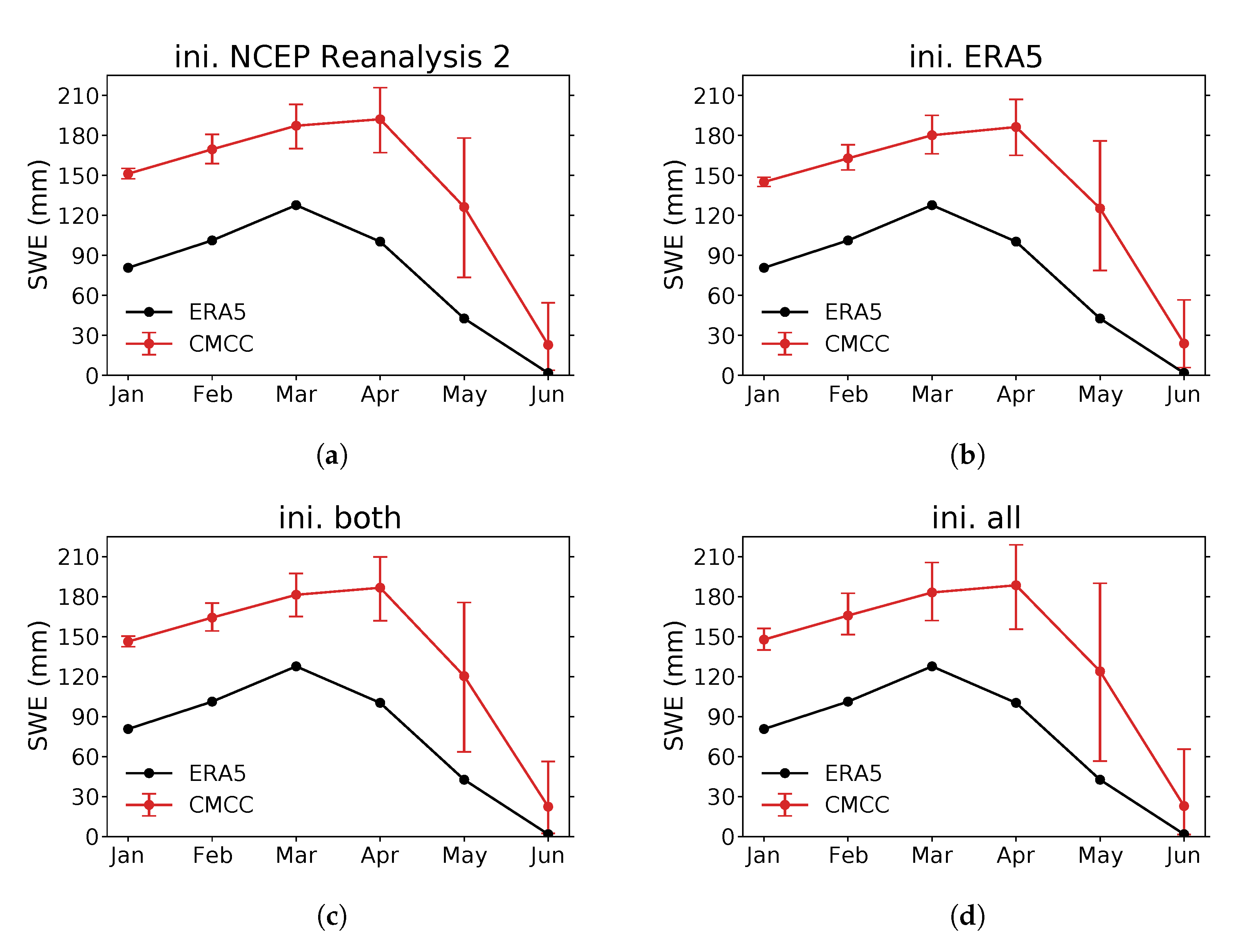
3.1. Initial Biases

The initial bias in the beginning of a forecast should be as low as possible. However, assimilating data to generate initial conditions is not trivial and differs from system to system, but in terms of initial land conditions, all five systems are generating them indirectly from nudged/assimilated atmospheric data or from offline land simulations, as explained earlier.

Figure 2 shows the biases of all five systems compared to ERA5 over Siberia of their common hindcast period from 1993 to 2016 for snow water equivalent (SWE), 2-m temperature (T2m), and total precipitation. Different colors in Figure 2 indicate different starting months, ranging from October to April, so that each first data point shows the initial bias. DWD and MF show similar biases for all three variables. While MF has overall lower biases, DWD has a lower bias at initial time with increasing error during the forecast (see, e.g., SWE and precipitation in winter or T2m in early winter in Figure 2). These analysis increments in the DWD system show a corrected initial state for SWE, T2m, and precipitation for each start month. Similar behavior can be seen for ECCC, whose initialization corrects the T2m in the early winter starting months. Small analysis increments, for example, for T2m at MF or SWE at ECCC (Figure 2), suggest a good model description of these variables. In contrast, the indirect/offline land initialization can also lead to analysis increments with higher, rather than lower, biases, as shown for SWE at ECMWF. However, most prominent are the increasing SWE biases from CMCC. With each starting month, the SWE bias increases until April, and also the negative T2m bias rises with the starting months in early winter and remains negative. This suggests that the cooling in CMCC in early winter and spring is due to the high initial snow overestimation (via snow–albedo effect and melting).

As already mentioned before, CMCC uses two reanalyses and their linear combination to generate initial conditions for its land variables. We sorted the members by their respective reanalysis initialization to obtain sub-ensembles. Dedicated plots for the sub-ensembles of the CMCC system are shown in Figure 3, which shows the SWE climatology for all simulations started in January, along with the ERA5 reference. All four types show the overestimation starting from January. Towards the end of spring, the absolute differences between the sub-ensemble means decrease due to melting. Besides a slightly higher overestimation in the NCEP2 sub-ensemble, there are no significant differences in SWE. This also applies to the ensemble spread between the indirectly initialized ensemble members by NCEP2, by ERA5, and by both. Thus, the additional data of NCEP2 cannot explain the general overestimation of initial snow in CMCC. A possible reason could be an imbalance between the initial snow and the multi-layer snow scheme.

After initialization, the parameterization generates the prognostic variables, which are discussed in the following.

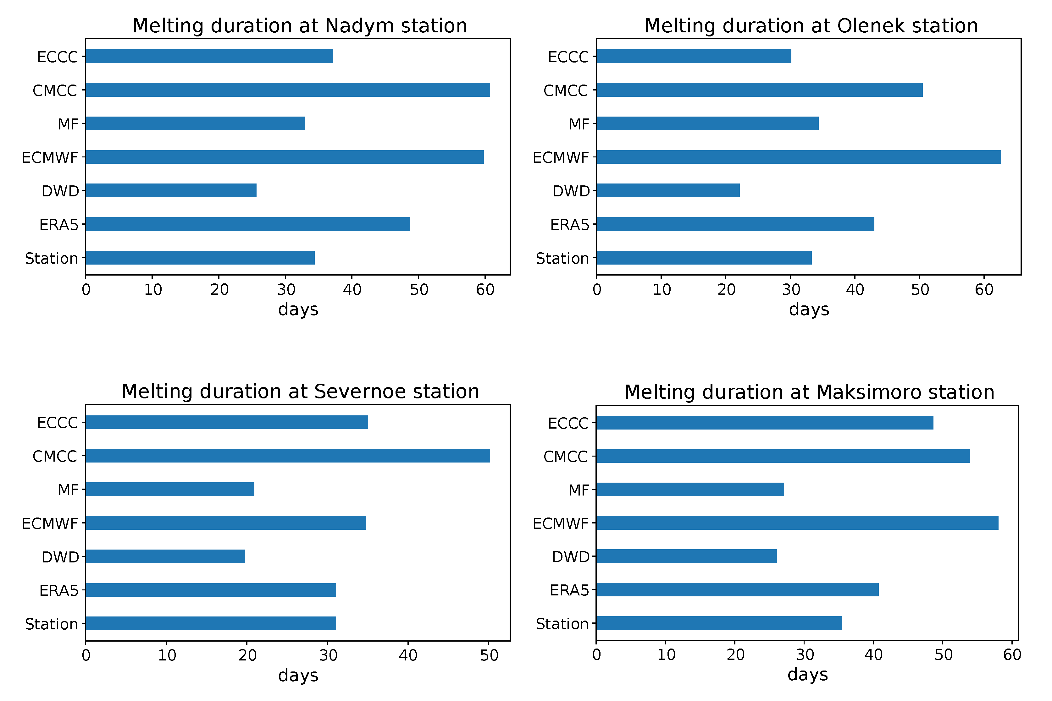
3.2. Snow Parameterization

The parameterization of snow can be divided into the accumulation phase, which mostly depends on precipitation and ambient air temperatures from the driving atmospheric model, and the melting phase, which depends on the melting formulation in the snow scheme, the incoming radiation, and turbulent heat fluxes [26]. However, we will focus on the general forecast performance and, more specifically, on the melting phase in the following.

Figure 4 shows the climatology of SWE, T2m, and total precipitation over Siberia from 1993 to 2016. Only simulations which started in October and February are shown, along with ERA5. In general, the accumulation phase (October to March) lasts longer than the melting phase (March to June), and the SWE maximum peaks in March. Already in October the domain average is below 0${}^{\circ }$C until April/May, and precipitation is highest in summer and lowest in February, with only about 22 mm. Additionally, we have the standard deviations for March in

Table 2. Inter-annual variability (standard deviation) for March (forecasted from February) of total snow water equivalent (SWE), monthly mean 2-m temperature (T2m), and monthly total precipitation over Siberia from 1993 to 2016 for the seasonal forecasting systems. Variabilities for March from ERA5 are also given.

Std. Dev.	SWE (mm)	T2m (K)	Total Precip. (mm)
ERA5	40.2	4.9	8.4
DWD	42.8	4.4	12.6
ECMWF	44.3	4.7	6.8
MF	61.7	5.8	9.4
CMCC	46.5	5.6	6.3
ECCC	34.8	4.7	5.5

, indicating the inter-annual variability. All systems except ECCC have similar or higher standard deviations for SWE compared to ERA5, whereas for T2m, the variabilities are closer to the reference.

From Figure 2 and Figure 4, we see an SWE overestimation from all systems except DWD and MF in late spring. The remarkable initial overestimations of SWE by CMCC have already been discussed in the previous section. However, additionally, during the simulations, these initial biases persist until the snow eventually melts completely at some time in late spring. The wintertime 2-m temperatures are overestimated by DWD, MF, and ECCC by 3 K to 4 K, whereas biases for March and April are small or negative. CMCC has an opposite pattern, with negative biases of about −3 K in late winter, and ECMWF is mostly close to the reference but with a negative bias in late spring. Towards spring, DWD and MF overestimate precipitation, with DWD having the highest bias. ECMWF and CMCC show only small precipitation underestimations during wintertime.

The general low biases of the ECMWF system compared to the ERA5 reference might be due to the similar underlying numerical model (ECMWF’s Integrated Forecast System); however, a comparison to MERRA-2 [27] reanalysis confirms this result (not shown).

In Figure 5 we show the Pearson correlation for SWE and T2m. Only DWD and ECMWF are shown as an example because the patterns from the other systems are mostly similar. The correlations for SWE are generally high for all systems. However, this does not apply to the correlations of the 2-m temperature forecasts, which are only high for the first month in each case. The ECMWF system is even worse for several months compared to the other systems, while its 2-m temperature bias (Figure 2) is the lowest. Compared to the 2-m temperature correlations, SWE correlations are degrading less, and some simulations even have a correlation coefficient higher than 0.5 after six months (e.g., ECMWF’s November run), but the magnitude and signs of the SWE biases of the systems differ significantly. The low correlations of all systems in 2-m temperature confirm the low predictability over continental regions such as Siberia for seasonal forecasts. The question remains as to why there is such a difference between the SWE and T2m correlation, or even between T2m bias and T2m correlation. Diro and Lin (2020) [1], who obtained similar results from subseasonal forecasting systems, suggested that this is caused by a weak snow–temperature coupling strength in the models.

Now we consider the melting process, first in the example of a single event and then over all hindcast years at four stations. The example of a melting event at Nadym station in spring 2013 is shown for a hindcast starting on 1 March from DWD and ECMWF with all of their ensemble members and together with reference data in Figure 6. With the beginning of the snowmelt or when the daily maximum 2-m temperature is larger than zero, the spread of SWE increases rapidly. As long as there is snow left, the 2-m temperature hardly exceeds the $0{}^{\circ }$C line because the melting process cools the ambient air. This is most pronounced in the DWD hindcasts, where it even seems to be a strict threshold. Similar observations can be made in the other years (not shown here).

At the stations, the snowmelt duration (from the maximum to one-third) lasts slightly more than one month, which is shown in Figure 7 at the bottom of each sub-figure. DWD and MF are melting too early and too fast at the selected stations (see Figure 7 and Figure 8), which can also be seen from their small underestimation in April and March (Figure 4), whereas ECMWF and CMCC are too late and are taking too long in the melting process. The reason might be the general overestimation from CMCC (see Figure 2), because it takes longer due to having more snow to melt. The gridded reference ERA5 also melts too slowly at three stations, but not as slowly as the previous two.

4. Summary and Conclusions

We compared the snow (SWE) and temperature (T2m) representation in five seasonal forecasting systems over western–central Siberia in terms of biases and correlations and their dependence on snow initialization and parameterization uncertainties. The uncertainties were attributed to initialization or parameterization errors by considering initial and emerging biases, diminishing correlation skills, and snowmelt performance.

The hindcasts by DWD’s and ECCC’s systems show positive initialization effects on SWE and T2m with analysis increments improving the results for the winter initial forecast months. However, in some systems, the initialization increases the initial biases (e.g., in CMCC’s system). The biases differ in sign and magnitude among the systems, although they use similar constraining analysis data and similar initialization approaches (land initialization via system simulations nudged to analyses or via offline land simulations forced by analyses). CMCC’s highly positive initial SWE biases amplify cooling in winter and spring. This positive bias was independent of the constraining analysis dataset.

The forecasting systems of CMCC and MF utilize multi-layer snow schemes, which should perform better than single-layer schemes, especially during the melting phase [10]. However, in the case of CMCC, the potential benefit could not emerge in the forecasts because of the too-large initial biases, which led to too-late and too-long snowmelt periods. This highlights the difficulties in balanced multi-layer snow initialization. MF’s system also did not perform more promising, which highlights the strong impact of the quality of the atmospheric forcing (especially of the radiation and turbulent heat fluxes in spring).

All systems show lower T2m than SWE correlation over Siberia. This has, for example, a negative impact on the systems’ ability to represent the melting onset in spring, which feeds back on temperature representation. The systems of MF and DWD forecast the snowmelt too early and too fast. In the case of DWD, this might be because of a parameterized constant snow density and an overestimation of sublimation (not shown).

Depending on the seasonal forecasting system discussed in this study, initialization or parameterization errors can be more dominant. Delayed hydrological and remote effects of the snow biases (e.g., contribution to soil moisture) and their impacts on the seasonal forecasts were not discussed in this paper, but are worth further investigation. In addition, the added value of complex multi-layer vs. single-layer snow schemes should be investigated more in-depth with seasonal modeling experiments. Our results indicate that the initialization methods of the systems’ land components should be improved and that special care has to be taken to initialize multi-layer snow. Additionally, we suggest seasonal hindcasting experiments using different snow initialization approaches (direct, indirect, or offline) to better disentangle the forecasting errors caused by snow initialization or snow parameterization.

References

1. Diro, G.T.; Lin, H. Subseasonal Forecast Skill of Snow Water Equivalent and Its Link with Temperature in Selected SubX Models. Weather Forecast. 2020, 35, 273–284. [Google Scholar] [CrossRef]
2. Lin, H.; Wu, Z. Contribution of the Autumn Tibetan Plateau Snow Cover to Seasonal Prediction of North American Winter Temperature. J. Clim. 2011, 24, 2801–2813. [Google Scholar] [CrossRef]
3. Sobolowski, S.; Gong, G.; Ting, M. Modeled Climate State and Dynamic Responses to Anomalous North American Snow Cover. J. Clim. 2010, 23, 785–799. [Google Scholar] [CrossRef]
4. Ruggieri, P.; Benassi, M.; Materia, S.; Peano, D.; Ardilouze, C.; Batté, L.; Gualdi, S. On the role of Eurasian autumn snow cover in dynamical seasonal predictions. Clim. Dyn. 2022, 58, 2031–2045. [Google Scholar] [CrossRef]
5. Henderson, G.; Peings, Y.; Furtado, J.C.; Kushner, P.J. Snow–atmosphere coupling in the Northern Hemisphere. Nat. Clim. Chang. 2018, 8, 954–963. [Google Scholar] [CrossRef]
6. Jeong, J.H.; Linderholm, H.W.; Woo, S.H.; Folland, C.; Kim, B.M.; Kim, S.J.; Chen, D. Impacts of Snow Initialization on Subseasonal Forecasts of Surface Air Temperature for the Cold Season. J. Clim. 2013, 26, 1956–1972. [Google Scholar] [CrossRef]
7. Li, F.; Orsolini, Y.J.; Keenlyside, N.; Shen, M.; Counillon, F.; Wang, Y.G. Impact of Snow Initialization in Subseasonal-to-Seasonal Winter Forecasts with the Norwegian Climate Prediction Model. J. Geophys. Res. Atmos. 2019, 124, 10033–10048. [Google Scholar] [CrossRef] [Green Version]
8. Lin, P.; Wei, J.; Yang, Z.L.; Zhang, Y.; Zhang, K. Snow data assimilation-constrained land initialization improves seasonal temperature prediction. Geophys. Res. Lett. 2016, 43, 11,423–11,432. [Google Scholar] [CrossRef]
9. Orsolini, Y.J.; Senan, R.; Balsamo, G.; Doblas-Reyes, F.J.; Vitart, F.; Weisheimer, A.; Carrasco, A.; Benestad, R.E. Impact of snow initialization on sub-seasonal forecasts. Clim. Dyn. 2013, 41, 1969–1982. [Google Scholar] [CrossRef]
10. Waliser, D.; Kim, J.; Xue, Y.; Chao, Y.; Eldering, A.; Fovell, R.; Hall, A.; Li, Q.; Liou, K.N.; McWilliams, J.; et al. Simulating cold season snowpack: Impacts of snow albedo and multi-layer snow physics. Clim. Chang. 2011, 109, 95–117. [Google Scholar] [CrossRef]
11. Cohen, J.; Entekhabi, D. Corrections to “Eurasian snow cover variability and northern hemisphere climate predictability”. Geophys. Res. Lett. 1999, 26, 1051. [Google Scholar] [CrossRef]
12. Singh, R.; Kishtawal, C.M.; Singh, C. The Strengthening Association Between Siberian Snow and Indian Summer Monsoon Rainfall. J. Geophys. Res. Atmos. 2021, 126, 1–22. [Google Scholar] [CrossRef]
13. Pulliainen, J.; Luojus, K.; Derksen, C.; Mudryk, L.R.; Lemmetyinen, J.; Salminen, M.; Ikonen, J.; Takala, M.; Cohen, J.; Smolander, T.; et al. Patterns and trends of Northern Hemisphere snow mass from 1980 to 2018. Nature 2020, 581, 294–298. [Google Scholar] [CrossRef] [PubMed]
14. Groisman, P.Y.; Gutman, G.; Shvidenko, A.Z.; Bergen, K.M.; Baklanov, A.A.; Stackhouse, P.W. Introduction: Regional Features of Siberia. In Regional Environmental Changes in Siberia and Their Global Consequences; Springer: Dordrecht, The Netherlands, 2013; pp. 1–17. [Google Scholar] [CrossRef]
15. Connolly, R.; Connolly, M.; Soon, W.; Legates, D.R.; Cionco, R.G.; Herrera, V.M. Northern Hemisphere Snow-Cover Trends (1967–2018): A Comparison between Climate Models and Observations. Geosciences 2019, 9, 135. [Google Scholar] [CrossRef] [Green Version]
16. Fröhlich, K.; Dobrynin, M.; Isensee, K.; Gessner, C.; Paxian, A.; Pohlmann, H.; Haak, H.; Brune, S.; Früh, B.; Baehr, J. The German Climate Forecast System: GCFS. J. Adv. Model. Earth Syst. 2021, 13, e2020MS002101. [Google Scholar] [CrossRef]
17. Johnson, S.J.; Stockdale, T.N.; Ferranti, L.; Balmaseda, M.A.; Molteni, F.; Magnusson, L.; Tietsche, S.; Decremer, D.; Weisheimer, A.; Balsamo, G.; et al. SEAS5: The new ECMWF seasonal forecast system. Geosci. Model Dev. 2019, 12, 1087–1117. [Google Scholar] [CrossRef] [Green Version]
18. Batté, L.; Dorel, L.; Ardilouze, C.; Guérémy, J.F. Documentation of the METEO-FRANCE Seasonal Forecasting System 8; Technical Report; Copernicus Climate Change Service: Reading, UK, 2021. [Google Scholar]
19. Gualdi, S.; Borrelli, A.; Davoli, G.; Masina, S.; Navarra, A.; Sanna, A.; Tibaldi, S.; Cantelli, A. The New CMCC Operational Seasonal Prediction System Issue TN0288 CMCC Technical Notes; Technical Report; CMCC: Lecce, Italy, 2020. [Google Scholar] [CrossRef]
20. Lin, H.; Merryfield, W.J.; Muncaster, R.; Smith, G.C.; Markovic, M.; Dupont, F.; Roy, F.; Lemieux, J.F.; Dirkson, A.; Kharin, V.V.; et al. The Canadian Seasonal to Interannual Prediction System Version 2 (CanSIPSv2). Weather Forecast. 2020, 35, 1317–1343. [Google Scholar] [CrossRef]
21. Hersbach, H.; Bell, B.; Berrisford, P.; Biavati, G.; Horányi, A.; Muñoz Sabater, J.; Nicolas, J.; Peubey, C.; Radu, R.; Rozum, I.; et al. ERA5 Monthly Averaged Data on Single Levels from 1979 to Present; Technical Report; Copernicus Climate Change Service (C3S), Climate Data Store (CDS): Reading, UK, 2019. [Google Scholar] [CrossRef]
22. Hersbach, H.; Bell, B.; Berrisford, P.; Biavati, G.; Horányi, A.; Muñoz Sabater, J.; Nicolas, J.; Peubey, C.; Radu, R.; Rozum, I.; et al. ERA5 Hourly Data on Single Levels from 1979 to Present; Technical Report; Copernicus Climate Change Service (C3S), Climate Data Store (CDS): Reading, UK, 2018. [Google Scholar] [CrossRef]
23. Hersbach, H.; Bell, B.; Berrisford, P.; Hirahara, S.; Horányi, A.; Muñoz-Sabater, J.; Nicolas, J.; Peubey, C.; Radu, R.; Schepers, D.; et al. The ERA5 global reanalysis. Q. J. R. Meteorol. Soc. 2020, 146, 1999–2049. [Google Scholar] [CrossRef]
24. Muñoz-Sabater, J.; Dutra, E.; Agustí-Panareda, A.; Albergel, C.; Arduini, G.; Balsamo, G.; Boussetta, S.; Choulga, M.; Harrigan, S.; Hersbach, H.; et al. ERA5-Land: A state-of-the-art global reanalysis dataset for land applications. Earth Syst. Sci. Data 2021, 13, 4349–4383. [Google Scholar] [CrossRef]
25. Mortimer, C.; Mudryk, L.; Derksen, C.; Luojus, K.; Brown, R.; Kelly, R.; Tedesco, M. Evaluation of long-term Northern Hemisphere snow water equivalent products. Cryosphere 2020, 14, 1579–1594. [Google Scholar] [CrossRef]
26. Kuusisto, E. Snow Accumulation and Snowmelt in Finland; Water Research Institute: Helsinki, Finland, 1984; Volume 55, pp. 1–149. [Google Scholar]
27. Gelaro, R.; McCarty, W.; Suárez, M.J.; Todling, R.; Molod, A.; Takacs, L.; Randles, C.A.; Darmenov, A.; Bosilovich, M.G.; Reichle, R.; et al. The Modern-Era Retrospective Analysis for Research and Applications, Version 2 (MERRA-2). J. Clim. 2017, 30, 5419–5454. [Google Scholar] [CrossRef] [PubMed]
Figure 1. Orography with height in meters of the Northern Hemisphere (≥40 N ). The black box (55–70 N , 65–115 E ) shows western–central Siberia, further referred to as Siberia. Red dots indicate the location of the four stations: Nadym ( 66 . 47 N , 72 . 67 E ), Olenek ( 68 . 50 N , 112 . 43 E ), Maksimoro ( 57 . 10 N , 104 . 97 E ), and Severnoe ( 56 . 35 N , 78 . 35 E ).
Atmosphere 13 01002 g001
Figure 2. Biases of SWE, 2-m temperature, and total precipitation averaged over the domain and all years of monthly data from hindcasts (1993 to 2016) with ERA5 as reference. Relative biases are shown for SWE and total precipitation, and absolute biases for 2-m temperature. Colors indicate different starting months.
Atmosphere 13 01002 g002
Figure 3. Average monthly SWE from 1993 to 2016 over Siberia from ERA5 (black) and CMCC (red). The red line represents the ensemble mean, and bars show the ensemble minimum and maximum averaged over the years and region. Panel (a) shows the sub-ensemble where only NCEP Reanalysis 2 was used to generate the indirect land initial conditions; (b) where only ERA5 was used; (c) a linear combination of both; and (d) the whole ensemble (sum of the previous).
Atmosphere 13 01002 g003
Figure 4. Climatology of SWE (a), 2-m temperature (b), and total precipitation (c) over Siberia with the reference (ERA5) and the seasonal forecasting systems from monthly data (1993–2016). Only starting months from October (solid) and February (dashed) are included.
Atmosphere 13 01002 g004
Figure 5. Pearson correlation for SWE and 2-m temperature of monthly data from hindcasts (1993 to 2016) with ERA5 as reference. Values were first averaged over the region before calculating the Pearson correlation coefficient. Colors indicate different starting months.
Atmosphere 13 01002 g005
Figure 6. Top: daily snow water equivalent (blue) and daily maximum 2-m temperature (red) for each ensemble member of DWD and ECMWF. Bottom: daily snow (blue), daily mean temperature (red line), and daily min/max temperature (red area) from ERA5 and Nadym station (snow given as snow depth).
Atmosphere 13 01002 g006
Figure 7. Days between the maximum and one-third of the snow depth at the grid-point closest to the station.
Atmosphere 13 01002 g007
Figure 8. Difference in days of the average melting date at the grid-point closest to the station from the seasonal forecasting systems and ERA5 compared to station data. The melt timing is defined by the time when one-third of the maximum snow depth is left.
Atmosphere 13 01002 g008